Optimizing line-plot size for personal laser scanning: modeling distance-dependent tree detection probability along transects
iForest - Biogeosciences and Forestry, Volume 17, Issue 5, Pages 269-276 (2024)
doi: https://doi.org/10.3832/ifor4588-017
Published: Sep 07, 2024 - Copyright © 2024 SISEF
Research Articles
Abstract
Personal laser scanning (PLS) systems are gaining popularity in forest inventory research and practice. They are primarily utilized on circular or compact rectangular sample plots to mitigate potential instrument drift and enhance tree detection rates, and a closed-loop scan path is usually implemented to achieve these objectives, ensuring thorough coverage of the plot. This study introduced a novel approach by applying the distance-sampling framework to PLS data collected during walks along line transects. Modeling the distance-dependent probability of tree detection using PLS coupled with automatic routines for point cloud processing aimed to ascertain the optimal width of line-plots to maximize tree detection rates. The optimized plots exhibited tree detection rates exceeding 99%, which facilitated accurate estimates of tree density, basal area, and growing stock volumes. This proposed method demonstrated considerable potential for data collection while walking along line transects in forests. For instance, the otherwise unproductive working time of field crews moving between systematically arranged sample plots can be utilized for additional data collection without generating additional costs. This innovative approach not only enhances operational efficiency but also establishes a foundation for further advancements to explore PLS applications in forest management practices.
Keywords
Personal Laser Scanning, Lidar, Forest Inventory, Distance Sampling, Line Transect Sampling, Tree Detection
Introduction
Forest inventories provide means and totals for measuring forest characteristics, such as the volume of growing stock, area of a certain forest type, and volume of dead wood or vegetation ([19]), which are crucial for decision-making in forest management ([29]). The Swedish botanist and forestry researcher Israel af Ström introduced systematic strip sampling in the 1830s and conducted the first regional-scale forest inventories, which remained popular for almost a century ([19]). National forest inventories (NFIs) based on modern statistical principles were implemented in Norway, Finland, and Sweden in 1919, 1920, and 1923 ([21]). In these NFIs, systematic strip sampling was replaced by a line-plot system wherein relatively small plots can be sampled along systematically arranged lines ([19], [45], [46]). Around 1990, many countries redesigned their NFIs and implemented systematic grid-based sample designs, consistent plot designs, and re-measurement intervals ([21]) that are still commonly used today.
Surprisingly, the instruments used in NFIs have changed marginally in recent decades, and mechanical and optical instruments, such as calipers, hypsometers, relascopes, and tape measures, are still commonly used today ([20], [21], [23]), although their usage is often labor-intensive and prone to measurement errors ([24], [25], [37]).
Terrestrial laser scanning (TLS) can collect high-resolution 3-dimensional (3D) data and represent stems and branches comprehensively; therefore, TLS-based estimates of tree attributes have reached an accuracy level that surpasses conventional measures ([50]). Despite these obvious advantages, TLS has so far hardly been used in forest inventory practices because the scanners are too heavy and complex to use ([28]). In addition to the pure scanning time, a substantial amount of working time is used to set up the scanner at different positions within a sample plot and to install artificial reference targets for co-registration of the scans ([16]). Personal laser scanning (PLS) systems overcome these limitations by enabling scanning during motion and registering point clouds using simultaneous localization and mapping algorithms ([15]). Consequently, the PLS point clouds are often noisier and less precise than the TLS point clouds ([3], [6]). However, they can derive accurate estimates of tree-level attributes from these datasets ([43]).
A major challenge in laser scanning operations is occlusion, which leads to incomplete point clouds ([8]) and consequently to the non-detection of several trees. The problem is especially pronounced when TLS is used in the single-scan mode ([38]), but also occurs in the multi-scan mode ([16], [24], [38]). In PLS applications, occlusion strongly depends on the scanning path and scan density ([3], [10], [48]). Bauwens et al. ([3]) recommended that the PLS path should end at the starting point (thereby creating a “closed loop”) to minimize instrumental drift and provide good coverage of the sample plot with minimum occlusion and range noise. Following these recommendations for the scan path layout, PLS was limited to relatively small and compact sample plots and experimental stands. Thus, in the forest inventory context, PLS has so far been used nearly exclusively in this setting type.
However, PLS principally allows data collection while walking along linear transects and can thus be used in a line-plot sampling system, which has rarely been used in recent years. However, in typical modern systematic grid-based sample systems, field crews walk along linear paths, for instance, when moving from one sample plot to the other, and no data are collected while walking. Thus, PLS principally provides the opportunity to collect data between sample plots without increasing the workload, simply by switching on the PLS scanner and carrying it from one sample point to another along a path that must be walked. However, this scanning layout violates all the recommendations on good PLS practices outlined above, and the non-detection of trees may become a serious challenge that must be carefully addressed.
Non-detection of sample objects is a common problem in wildlife ecology; thus, a distance sampling framework ([4], [5]) was developed for applications in this field ([42]). The main objective of distance sampling is to use the observed distances between the observer and detected objects of interest to fit a detection function that describes the decrease in detectability with increasing distance ([42]). In the forest inventory context, distance sampling has been successfully used for sampling deadwood ([34], [36]), habitat trees ([2], [11]), and low-abundance tree species ([22]), and to correct non-detection in angle-count sampling ([35]), single-scan TLS ([1], [12]), and multi-scan TLS ([38], [39]).
In this study, the potential of PLS-based data collection along lines was evaluated regarding the possibility of collecting additional data during systematic grid-based forest inventories using the walking time for PLS scans and without spending any additional working time on other plots in the field. To the best of our knowledge, this is the first study to adopt the distance-sampling framework for PLS data. We used a GeoSLAM ZEB Horizon® (GeoSLAM Ltd., Nottingham, UK) PLS system to collect data along 23 transects with a total length of 4157.7 m in two stands that were fully mapped for reference. Three different detection functions were evaluated, a correction for non-detection was developed, and recommendations for an optimal line-plot width were also made.
The main objectives of this study were to (i) test the applicability of PLS along transects, (ii) determine the optimal width of line plots to maximize tree detection rates with PLS using the distance sampling framework, and (iii) optimize line plot length to facilitate precise estimates of tree density, basal area, and growing stock volume.
Materials and methods
Experimental stands and reference data
The survey was conducted at two fully mapped experimental stands (Fig. 1). Position, diameter at 1.3 m height (dbh), and height of all trees having a dbh ≥ 5 cm were manually measured for reference. Reference stem volume was calculated using an established stem form function ([30]) with height and dbh as input variables.
Fig. 1 - Location of the two experimental stands (BuLae and 30k) in Austria.
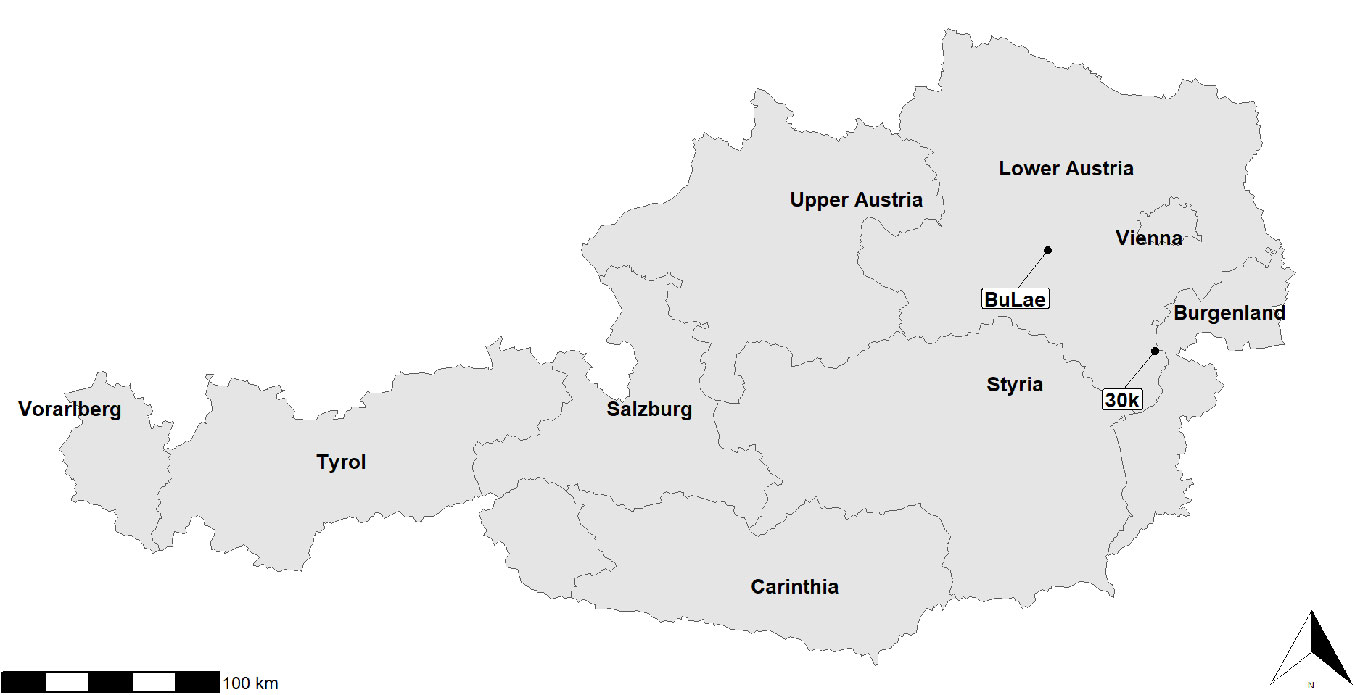
The first experimental stand with an area of 4.88 ha located near the village of Kreisbach, Lower Austria (48.10° N, 15.63° E), was referred to as “BuLae”. The stand was mature and characterized by an uneven mixture of 90% beech (Fagus sylvatica) and 6% larch (Larix decidua), with no understory and only sparse natural regeneration. The mixed tree species included 2% spruce (Picea abies), 1% oak (Quercus spp.), and less than 1% other species, mainly fir (Abies alba), hornbeam (Carpinus betulus), lime (Tilia spp.), and ash (Fraxinus excelsior). The total number of trees was 2867 corresponding to a density of 588.5 trees ha-1. The median tree height was 30.2 m (min = 3.4 m, max = 43.5 m), and the median dbh was 29.3 cm (min = 5.0 cm, max = 68.0 cm). Stand basal area was 216.1 m2 (= 44.3 m2 ha-1) and total volume of the growing stock was 3203.3 m3 (= 656.4 m3 ha-1).
The second experimental stand with an area of 4.08 ha located in the BOKU University training forest near Hochwolkersdorf Village in Lower Austria (47.68° N, 16.29° E) was referred to as “30k”. This stand included 1789 trees, with a corresponding density of 438.5 trees ha-1. The stand is characterized by high structural diversity, including a spatially irregularly distributed understory and regeneration. Diversity of tree species was comparatively high for the area, with 38% spruce (Picea abies), 38% beech (Fagus sylvatica), 15% fir (Abies alba), 5% pine (Pinus sylvestris), 4% larch (Larix decidua), and <1% of other broadleaf species. Natural regeneration occurred in irregularly arranged clusters comprising approximately 90% beech and 10% fir. The median tree height was 29.7 m (min = 5.4 m, max = 40.9 m), and the median dbh was 36.3 cm (min = 9.9 cm, max = 67.3 cm). Stand basal area was 191.5 m2 (= 46.9 m2 ha-1) and the total volume of the growing stock was 2686.7 m3 (= 658.8 m3 ha-1).
Scan data collection and analysis
Scan data collection was performed under defoliated conditions in winter 2021/22 using a GeoSLAM ZEB Horizon® (GeoSLAM Ltd., Nottingham, UK) PLS system that uses the simultaneous localization and mapping technique. The scanner has a maximum range of 100 m and collects 300.000 scan points s-1 with an accuracy of ± 6 mm ([14]).
The transects were aligned parallel to each other, with a spacing of approximately 20 m. The start and end points of each transect were located on opposing stand borders (open loops). Nine transects were scanned in BuLae, having a mean length of 284.3 m (minimum length = 122.6 m, maximum length = 461.0 m), and 14 transects were scanned in 30k, having a mean length of 115.5 m (minimum length = 102.7 m, maximum length = 130.0 m). The transect lengths resembled the typical distances between forest inventory sample points.
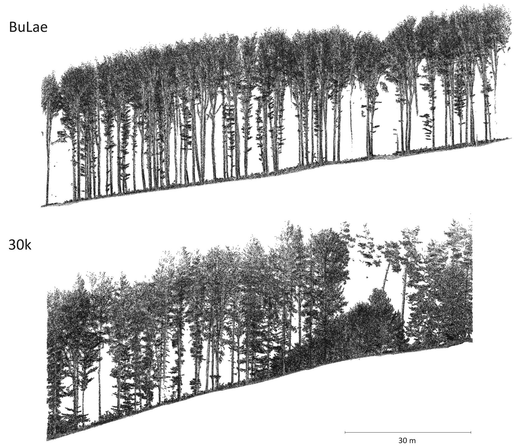
The raw scan data were converted into point clouds in the .laz format using the software GeoSlam HUB ver. 5.3 ([13]) in a local coordinate reference system for each transect separately (Fig. 2). In addition to the point cloud, the trajectory of the instrument (i.e., walking path of the observer) was exported in the .csv format with the same coordinate reference system as the corresponding point cloud. The point clouds were then processed in R language and environment for statistical computing ([33]) using fully automatic routines for tree detection, tree segmentation, and tree variable estimation implemented in the R-package “treeX” ([44]). In a preparatory step, the point cloud was cropped, normalized, and filtered, leaving only vegetation hits. Tree positions were then automatically detected through multi-stage, density-based clustering, and the diameter at breast height was estimated by fitting a circle to the trunk cross-section at a height of 1.3 m ([37], [15]). The point cloud was then voxelated and the detected tree positions served as starting points for a 3D region-growing algorithm for automatic tree segmentation ([43]), allowing the height of each individual tree to be estimated as the difference between the highest and lowest z-values of voxels belonging to the tree. The tree volume was then estimated using the same stem form function ([30]) as the reference data to ensure a fair comparison. Finally, trees with dbh < 5 cm were removed from the tree list, as this was also the caliper threshold in the reference data.
Fig. 2 - Exemplary section of the point cloud recorded along a transect for the two experimental stands.
Orthogonal distances between the tree positions and the transect were calculated, and distance sampling analysis was conducted using the R package “Distance” version 1.0.7. ([27]).
Distance sampling approach
We used the classic line transect sampling approach of the distance sampling framework to estimate the number of trees per unit area. A brief description of the procedure is given below, for more details we refer to Buckland et al. ([4], [5]).
Using the classic line-plot sampling approach, m number of plots with a constant width 2ω were sampled along a line. With li being the length of the i-th plot, the total length of all plots was then L=∑i=1nmli. Thus, all n trees within an area of size α=2ωL were sampled, and the density D, i.e., the number of trees per area unit, was estimated using the following equation (eqn. 1):
However, this implied perfect detectability of trees, and any missed trees will lead to a non-detection bias. Using laser scanning systems and automatic routines for tree detection, the probability of detecting a tree decreases with increasing distance between the scanner and the tree, owing to decreasing point density and obstruction ([1], [12], [38], [39]). Thus, only a proportion Pa of the trees located within an area of size a was detected. If Pa can be estimated by hat{P}a, D can be estimated as follows (eqn. 2):
But how can Pa be estimated? According to Buckland et al. ([4]), the basic concept of line transect sampling is that the detectability of objects decreases with increasing distance x between the transect and the object of interest (a tree in our application). By fitting a distance-dependent detection function g(x) to the normalized density of observed objects at different distances (0 ≤ x ≤ ω), and assuming certain detection of objects located directly on the transect [g(0) = 1], the mean detection probability within a strip of area a can then be estimated as (eqn. 3):
The density estimator (eqn. 2) then becomes (eqn. 4):
The standard error of hat{D} can be estimated using the delta method as described below ([41] - eqn. 5):
The detection function g(x) is typically represented by a parametric function and can be fitted using maximum-likelihood techniques ([4], [5]). Because parametric detection functions have proven to be robust and provide sufficient flexibility, and because their inference is straightforward, they are generally preferred over nonparametric alternatives ([32]).
The best detection function was selected from nine candidate functions based on the minimum Akaike Information Criterion (AIC), for both stands separately. The candidate functions comprised a key function and a first-order series expansion (Tab. 1).
Tab. 1 - Combinations of key functions and series expansions used as candidate models for estimating the detection function. is the scale parameter of the detection function, b is the shape parameter of the detection function, y is the coefficient of the series expansion, Hj is the jth Hermite polynomial, and aj is set to zero if term j is not used in the model.
| Key function | Series expansion |
|---|---|
| Uniform: hat{g}(x) = 1/ω | None Cosine: ∑mj=1 aj · cos(jπy/ω) ∑ Simple polynomial: ∑mj=1 aj (y/ω)2j |
| Half-normal: hat{g}(x) = exp(-(x²/2σ²)) | None Cosine: ∑mj=2 aj · cos(jπy/ω) Hermite polynomial: ∑mj=1 aj H2j (y/σ) |
| Hazard-rate: hat{g}(x) = 1-exp(-(x/σ)-b) | None Cosine: ∑mj=2 aj · cos(jπy/ω) Hermite polynomial: ∑mj=1 aj H2j (y/σ) |
The distance sampling approach allowed the correction of the number of missed trees and provided estimates for the number of trees per unit area. However, forest managers are normally more interested in stand basal area (BA) and volume of growing stock (V). As tree size can possibly affect detection probability, larger trees might be overrepresented in the sample (size bias); therefore, estimates of BA and V derived from the distance sample might also be biased. The size bias can be principally corrected using regression techniques ([4], [34]); however, this introduces a new source of uncertainty. Moreover, this approach only provides estimates for the totals of BA and V but no single-tree information. Therefore, we did not follow this approach and instead used the shape of the detection function to determine the optimal line-plot width, that is, the maximum line-plot width where tree detection is certain and non-detection becomes irrelevant.
Determination of optimal line-plot size
Detection functions often show a noticeable shoulder, i.e., a range of distances from the line for which the slope g’=0. Thus, the shoulder indicates the range of distances at which a tree can be detected with certainty ([31]). We used this characteristic to estimate the optimal line-plot width, i.e., the maximum plot width for which the detectability of trees is certain, by determining the greatest distance ωopt where g’<0.005. We used this constraint instead of g’=0 because the numerically calculated values of g’(x) might have been influenced by the rounding errors of the parameter estimates. The corresponding optimal line-plot width was then estimated as 2ωopt, because trees could be detected on the left and right side of the line. We then truncated the distance sampling data at ωopt, such that every transect could be treated as a line-plot of area ai = 2ωopt li.
As the sampling units are of unequal size (ai ≠ const), the population mean of any response variable Y (D, BA, V) cannot be estimated as the sample mean over the m line-plots because the observations yi are correlated with ai. Thus, we estimated the population mean of any response variable per unit area hat{Y} using the following ratio estimator (eqn. 6):
where hat{bar{Y}}R is model unbiased only in case of a linear relationship of the form yi = βai + εi between y and a, where the regression line is passing through the origin with positive slope β, and the random error εi is independently and identically normal distributed. Otherwise, hat{bar{Y}}R is approximately unbiased for sufficiently large sample sizes ([7], [9]).
Using the finite population approach, the standard error (SE) for hat{bar{Y}}R was estimated as (eqn. 7):
where f is the sampling fraction, bar{a} is the mean line-plot area, sy2 is the sample variance of the target variable over line-plots, sa2 is the sample variance of the line-plot areas, and say is the covariance between the line-plot area and the target variable ([7]). As the term m·bar{a} = const for any given value of f, m has no direct influence on the estimated SE. However, sy2 and say depend on the distribution of line-plot sizes ai, and therefore, for a fixed sampling fraction f, also on m.
To assess the impact of different lengths and numbers of line-plots at a constant sampling fraction, we divided the individual transects into segments ranging from 1 to 50 m in length. Segments at the stand edges may have been shorter because of the irregular shape of the stands. To capture the effect of different starting points on segmentation, the starting points were varied on a 1 × 1 m grid.
Accuracy of tree detection
Eqn. 6 and eqn. 7 yield (approximately) unbiased estimates only when all trees within the sample plots are detected and no false detection occurs. Although the distance-sampling model indicated total detectability within the plot, it did not provide any false detection information. Thus, the accuracy of the tree detection was evaluated by comparing the automatically detected tree positions with the reference data. The automatically detected tree positions were assigned to the reference positions using a point assignment algorithm ([17], [49]), with position deviations of up to 0.5 m permitted. We then assessed the accuracy of tree detection in terms of the omission error, o (eqn. 8), commission error c (eqn. 9), and overall accuracy acc (eqn. 10) to evaluate the accuracy of the model prediction and the assumption that there were no false-positive detections:
where nmatch is the number of correctly found reference trees, nref is the total number of reference trees, nfalsepos is the number of tree positions which could not be assigned to an existing tree in the reference data, and nextr is the number of automatically detected tree positions (nmatch + nfalsepos). The omission error o (%) measures the percentage of undetected trees, commission error c (%) measures the percentage of falsely detected tree locations, and overall accuracy acc (%) is a combination of the latter two metrics and represents a global quality criterion. The detection rate, measuring the percentage of correctly identified trees, is given by dr = 100% - o (%).
Results
Distance sampling approach
All candidate functions were fitted to the observed distances between trees and transects obtained from the PLS data and compared in terms of the minimum AIC.
The detection functions with the hazard rate key generally performed the best for both stands; however, their advantage over the other functions was much more pronounced for BuLae than for 30k. While the uniform detection functions performed clearly inferiorly to the hazard rate functions in both stands, the half-normal detection functions almost reached the AIC level of the hazard rate functions in 30k, whereas they were clearly inferior in BuLae (Tab. 2).
Tab. 2 - Akaike information criterion (AIC) and parameter estimates for the different candidate detection functions and experimental stands. Emphasized: The hazard rate detection function that was finally selected.
| Detection function | BuLae | 30k | ||||||
|---|---|---|---|---|---|---|---|---|
| AIC | σ | b | SEcoef | AIC | σ | b | SEcoef | |
| Uniform | 7728.2 | NA | NA | NA | 4654.5 | NA | NA | NA |
| Uniform + Cosine | 6371.1 | NA | NA | 0.998 | 4106.3 | NA | NA | 0.979 |
| Uniform + Polynomial | 7127.7 | NA | NA | -0.997 | 4439.1 | NA | NA | -0.994 |
| Half-normal | 6230.7 | 3.664 | NA | NA | 4085.6 | 4.241 | NA | NA |
| Half-normal + Cosine | 6217.9 | 3.400 | NA | -0.219 | 4085.4 | 4.124 | NA | -0.096 |
| Half-normal + Polynomial | 6219.6 | 2.878 | NA | -0.270 | 4087.1 | 4.356 | NA | -0.359 |
| Hazard rate | 6198.7 | 4.558 | 4.363 | NA | 4084.8 | 5.360 | 4.276 | NA |
| Hazard rate + Cosine | 6200.7 | 4.558 | 4.363 | 0.000 | 4087.0 | 6.021 | 5.284 | 0.203 |
| Hazard rate + Polynomial | 6199.3 | 4.483 | 3.783 | 0.342 | 4086.6 | 5.665 | 3.628 | 0.228 |
Adding polynomial or cosine series expansions did not result in better performance of the hazard rate function. Thus, the hazard rate detection function without series expansion and with parameter estimates according to Tab. 2 was selected as the final model based on the minimum AIC for both experimental stands. The function showed a strong shoulder for both stands (Fig. 3) ranging from 0 m to approximately 3 m, followed by a steep decline to approximately 8 m. For greater distances, the function asymptotically approached the x-axis.
Fig. 3 - Hazard rate detection function (red line) fitted to the histogram of detected tree frequency in the different distance classes.
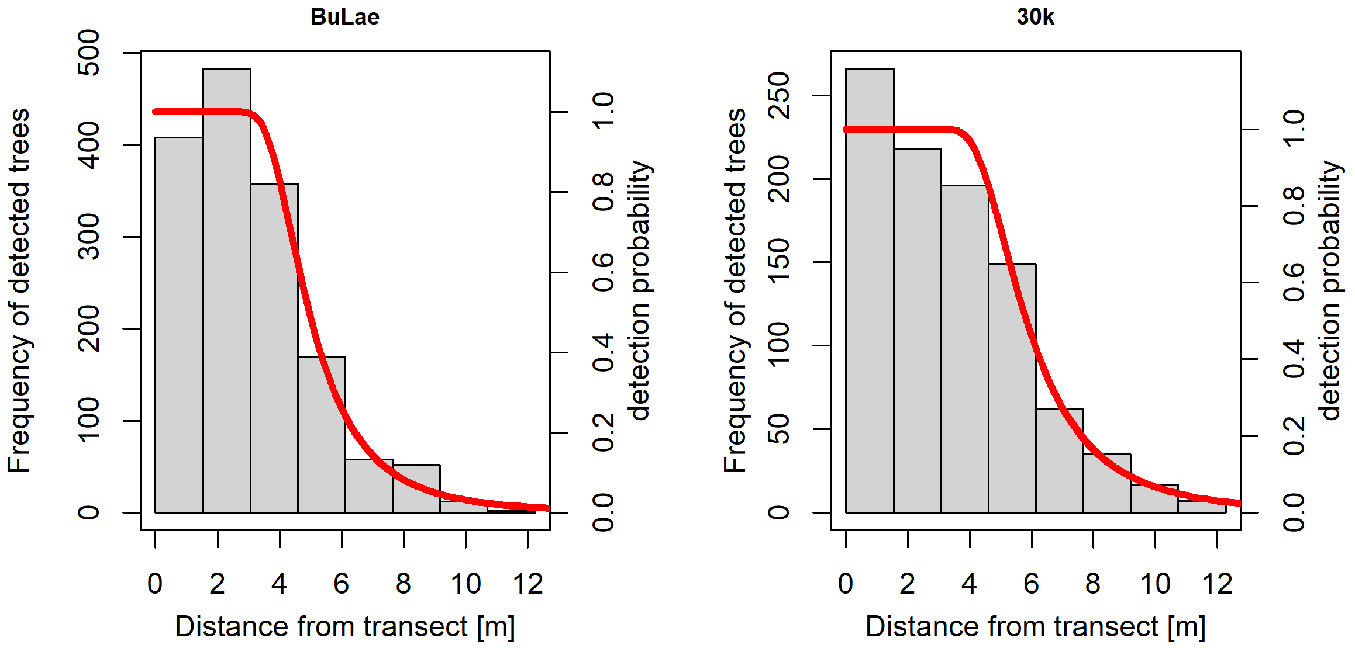
The estimated tree densities (eqn. 4) ± SE (eqn. 5) was 556.9 ± 18.8 trees ha-1 for BuLae, and 462.7 ± 52.0 trees ha-1 for 30k. The corresponding reference values of 587.5 and 438.5 trees ha-1 were within the respective confidence intervals of the estimates (Tab. 3). The relative standard error was 9.3% for BuLae and 4.1% for 30k.
Tab. 3 - Tree density, reference values (Ref), estimates (Est), standard errors (SE), and 95% confidence intervals (95%-CI) for both stands.
| Stand | Metric | Ref | Est | SE | 95%-CI |
|---|---|---|---|---|---|
| BuLae | Total number of trees in the stand | 2867.0 | 2717.5 | 253.9 | [2198.2-3359.5] |
| Number of trees ha-1 | 587.5 | 556.9 | 52.0 | [450.5-688.4] | |
| 30k | Total number of trees in the stand | 1789.0 | 1887.7 | 76.7 | [1737.5-2050.9] |
| Number of trees ha-1 | 438.5 | 462.7 | 18.8 | [425.9-502.7] |
Volume and basal area were not estimated with this approach for the reasons explained above (section “Distance sampling approach”).
Line-plot approach
The width of the detection function shoulder was numerically determined as the greatest distance ωopt where g’(ωopt) = 0.005. The closed-form derivative (eqn. 11) exited for the hazard rate function, such that g’ was determined without further numeric approximation:
The greatest distance ωopt was 2.86 m for BuLae and 3.33 m for 30k. Consequently, line-plots of width 2ωopt (5.72 m for BuLae and 6.66 m for 30k) were observed along the transect lines.
With the given sampling fraction, the mean standard error for the target variable V was minimal for line-plot lengths of 9 m for BuLae and 12 m for 30k (Fig. 4).
Fig. 4 - Relative standard error (relSE) for the estimated volume per ha V depending on the individual line-plot length. Total line-plot length was constant (2558.7 m for BuLae and 1617 m for 30k). The solid black line indicates the mean relSE for the corresponding plot length, while the gray area indicates the variability of relSE estimates based on the starting point of the systematic grid.
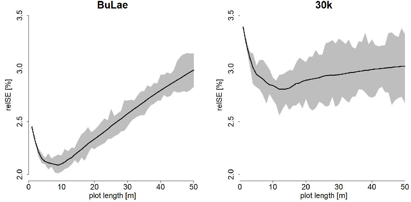
Consequently, line-plots of size 9 × 5.72 m and 12 × 6.66 m were used to assess the precision of the target variable estimates for BuLae and 30k respectively.
For BuLae, target variable estimates were 571.9 trees ha-1 for density, 45.76 m2 ha-1 for basal area, and 642.7 m3 ha-1 for volume, while for 30k, the estimates were 571.9 trees ha-1 for density, 45.76 m2 ha-1 for basal area, and 642.7 m3 ha-1 for volume. Reference values of all target variables were within the corresponding 95% confidence interval for each experimental stand (Tab. 4). The precision of the estimates was substantially higher for BuLae than for 30k (Tab. 4).
Tab. 4 - Point estimates (Est), reference values (Ref), standard errors (SE), and 95% confidence intervals (95%-CI) for both stands, and for three target variables D (trees ha-1), BA (Basal area m2 ha-1), and V (Volume, m3 ha-1). (N): number of plots.
| Stand | Plot size (m) |
N | Response variable | Ref | Est | SE | 95%-CI |
|---|---|---|---|---|---|---|---|
| BuLae | 9 × 5.72 | 294 | D (trees ha-1) | 587.5 | 571.9 | 11.3 | [553.3-590.4] |
| BA (Basal area, m2 ha-1) | 44.28 | 45.76 | 0.96 | [44.18-47.34] | |||
| V (Volume, m3 ha-1) | 656.4 | 642.7 | 12.9 | [620.5-664.8] | |||
| 30k | 12 × 6.66 | 149 | D (trees ha-1) | 438.5 | 456.7 | 13.7 | [434.1-479.3] |
| BA (Basal area, m2 ha-1) | 46.94 | 45.77 | 1.28 | [43.65-47.89] | |||
| V (Volume, m3 ha-1) | 658.8 | 650.6 | 18.2 | [620.5-680.7] |
Accuracy of tree detection
The accuracy of target variable point estimates (Tab. 4) depended on the assumption that trees within line-plots of width 2ωopt were detected with certainty, as indicated by the distance sampling model.
To evaluate the validity of the model results, the accuracy of tree detection was assessed based on reference data (Tab. 5). The true detection rates exceeded 99% for both stands (omission errors <1%), and the number of false detections was negligible (commission errors <0.4%). The overall accuracies were 98.88% for BuLae and 98.83% for 30k.
Tab. 5 - Accuracy of tree detection within sample line-plots of optimal width 2ωopt.
| Stand | BuLae | 30k |
|---|---|---|
| Plot width, 2ωopt (m) | 5.72 | 6.66 |
| Omission error, o (%) | 0.91 | 0.78 |
| Commission error, c (%) | 0.21 | 0.39 |
| Detection rate, dr (%) | 99.07 | 99.23 |
| Overall accuracy, acc (%) | 98.88 | 98.83 |
Discussion
Accuracy and precision of forest inventory target variable estimates
The classic line transect sampling approach is primarily designed to estimate detection probability and tree density. We used this approach and achieved a standard error of 52.0 trees ha-1 for BuLae and 18.8 trees ha-1 for 30k (Tab. 3). Contrastingly, the optimized line-plot sampling technique demonstrated a notable reduction in standard errors, resulting in values of 11.3 and 13.7 trees ha-1 for BuLae and 30k, respectively (Tab. 4). This improvement can be attributed to the ability of the method to precisely estimate the strip width where detection is certain, leveraging the precise measurement of the width of the shoulder of the detection function. Conversely, the conventional approach struggles to model the decrease in detectability with increasing distance from a line with the same level of precision.
The point estimates obtained using the optimized line-plot sampling for the forest inventory target variables (Tab. 4) were approximately unbiased for two reasons: (i) the residuals from the linear models between yi and ai and are not independently and identically distributed, rendering eqn. 6 only approximately unbiased; (ii) the detectability of trees in the optimized line-plots was not perfect (Tab. 5) with <1% of the trees missed, thereby introducing a minor negative bias.
The precision of the point estimates for the forest inventory target variables was greater for BuLae than for 30k stand plot. This finding was expected, considering that 30k possesses a more intricate stand structure than BuLae, and that the sampling fraction was higher in BuLae than in 30k.
The open loop scan path did not cause any problems regarding instrumental drift on the observed transects of length varying between 102.7 and 461.0 m, and tree detection was almost perfect on line-plots with optimized width.
The sampling fraction was very high in both stands. In 30k, the total length of the 14 transects was 1617.0 m, and the line-plot width was 6.66 m, yielding a total sample plot area of 10.769 m2, or 26.4% of the total stand area (4.08 ha). In BuLae, the total length of the 9 transects was 2558.7 m, and the line-plot width was 5.72 m, yielding a total sample plot area of 14.636 m2, or 30.0% of the total stand area (4.88 ha). This high sampling fraction is infeasible in most practical applications. However, providing an efficient methodology for obtaining standard-level volume estimates was not the focus of this study. Instead, we only used the two experimental stands for a comprehensive reference and focused on the potential of PLS-based data collection along lines with regard to the possibility of collecting additional data during systematic grid-based forest inventories. This topic has been further discussed below.
Algorithms for point cloud processing
The distance-sampling approach assumes the total detectability of trees in close proximity to the line transect. However, depending on the algorithms applied for point-cloud processing and tree detection, trees that are visible in the point cloud may remain undetected. For example, the lower part of the stem could be obstructed by natural regeneration or other vegetation types (omission errors). Conversely, algorithms may misinterpret non-tree objects as trees, such as when the branches of fallen trees are oriented vertically (commission error).
This study did not focus on algorithm development, improvement, or comparison of different algorithms. Instead, the emphasis was on applying PLS to an operational setting. Therefore, we utilized a single set of existing algorithms for data analysis. The omission and commission error rates achieved with these algorithms on the line-plots provided very little room for improvement, given that detectability was nearly perfect (>99%) and commission errors were negligible (<0.5%). However, alternative algorithms for point cloud processing can yield detection functions with a broader shoulder, allowing for the sampling of wider line-plots, which is desirable.
Selection of detection function
Parametric detection functions are typically favored over nonparametric alternatives owing to their robustness, sufficient flexibility, and straightforward inferential procedures ([32]). Hence, we exclusively employed parametric candidate functions, and our findings suggested that these functions are adequate for modeling the distance-dependent detectability of trees with PLS.
The choice of hazard rate detection function without series adjustments was determined using the minimum AIC. However, particularly in the case of stand 30k, the differences in AIC values (ΔAIC) were occasionally marginal. For instance, ΔAIC was 0.6 for the hazard rate function without series adjustments compared to the half-normal function with cosine adjustments. Akaike’s rule of thumb is that two models are essentially indistinguishable if ΔAIC ≤ 2, that 2 < ΔAIC ≤ 4 indicates moderate evidence of a difference in the models, and that ΔAIC > 4 indicates strong evidence of a difference in the models. When the model selection is uncertain, we recommend adhering to a simpler model because it is easier to explain and less susceptible to issues with shape constraints that may arise when employing series expansions. Therefore, though the AIC for the half-normal function with cosine adjustments was slightly lower than that for the hazard rate function without series adjustments, we would still prefer the latter model.
Possible further model developments
Omission errors in proximity to the transect were minimal, justifying the use of the classic line transect sampling approach. The principal advantage of this method is its ability to self-adjust to different sighting conditions using flexible detection functions. Thus, the method can be applied to other research areas without the need for intense reference data collection.
The virtual absence of omission errors in close proximity to the transect may appear unexpected, because significant omission errors were observed near the scanner using single-scan TLS and the same point cloud processing algorithms ([38]). However, PLS offers a significant advantage by scanning not only from a single point, but also along a line, thereby avoiding considerable shadowing. If shadowing and non-detection occur near the transects during further investigation, a correction can be implemented for imperfect detectability that was originally developed for point-transect sampling in conjunction with TLS ([38]). However, this approach requires reference data for model fitting and may have limited practical applicability.
We employed the classic line transect sampling approach exclusively to estimate the detection probability and, consequently, tree density. However, it is theoretically possible to regard each tree as a cluster of volume units with a cluster size, enabling the estimation of the total volume per hectare by multiplying the estimated cluster density by an estimate of the mean cluster size ([34]). Because the detection probability of large clusters may differ from that of smaller clusters, modeling the expected size of the detected clusters as a function of the distance-dependent detection probability can correct for the potential size bias. This correction addresses the issue that would arise if the mean cluster size was simply estimated as the sample mean of all observed clusters ([4]). While this approach has proven successful in the context of deadwood sampling ([34]) and TLS in single-scan mode ([1]), it has a fundamental limitation: the correction for non-detection is applicable only to tree density and total volume. Additional details, such as diameter distribution, spatial arrangement of trees, and resulting interactions, cannot be obtained using this analytical method. Consequently, our emphasis was on determining the optimal line-plot width because line-plots provide an opportunity to evaluate the aforementioned supplementary information.
Possible areas of application
Many NFIs utilize systematically arranged clusters of multiple measurement units. These clusters are typically spaced several kilometers apart and require field crews to commute between them by car. However, the gaps between the measuring units within a cluster are considerably smaller, necessitating field crews to walk these distances. For instance, the distances between measuring units within a cluster were 120 ft (36.58 m) in the US NFI ([26]), 150 m in the German NFI ([18]), 200 m in the Austrian NFI ([40]), and 250-450 m (depending on the ecoregion) in the Finnish NFI ([47]). This study demonstrates the applicability of PLS to line-plots of comparable length (102.7-461.0 m). The field operator was required to carry the PLS system while walking along a line through the forest and pressing the instrument’s start/stop button at the beginning and end of the transect. Consequently, we believe that it is feasible to integrate PLS-based line-plot sampling into existing large-scale forest inventories without requiring additional time in the field.
This study was constrained by the limited representation of the observed forest types, as it focused only on two stands. Consequently, further research should be conducted to investigate how various stand types and vegetation conditions (foliated versus defoliated) influence the detection function. The effectiveness of employing a global model adjusted for local visual conditions through the inclusion of covariates, compared with utilizing independent models tailored to specific areas, remains uncertain. Despite these ambiguities and considering the long-standing success of distance sampling, we contend that overcoming these challenges is feasible. Extending the method to diverse conditions is plausible for determining the optimal plot width for accurate assessment.
Conclusion
The distance sampling framework proved to be suitable for determining the optimum width for line-plots to be sampled with PLS, such that non-detection errors on these plots could be virtually eliminated (<1%). A posteriori segmentation of the line-plots into smaller units evidently reduced the standard error. This enabled the application of PLS to line-plots and ensured the accurate and precise estimation of tree density, basal area, and volume. Further investigations are required to validate these findings in various forest types. Nonetheless, we are confident that the methodology introduced in this study allows the integration of PLS-based line-plot sampling into existing forest inventories relying on systematically aligned sample plots. In the field, crews can seamlessly carry the PLS device while moving between sampling points, facilitating additional data collection without extending working hours.
References
Gscholar
Gscholar
CrossRef | Gscholar
Online | Gscholar
CrossRef | Gscholar
CrossRef | Gscholar
CrossRef | Gscholar
Gscholar
Gscholar
Gscholar
Gscholar
Authors’ Info
Authors’ Affiliation
Andreas Tockner 0000-0001-6833-6713
Ralf Krassnitzer
Sarah Witzmann 0000-0002-4882-5920
Christoph Gollob 0000-0002-7036-5115
Arne Nothdurft 0000-0002-7065-7601
University of Natural Resources and Life Sciences, Vienna - BOKU, Department of Forest and Soil Science, Institute of Forest Growth, Vienna (Austria)
Corresponding author
Paper Info
Citation
Ritter T, Tockner A, Krassnitzer R, Witzmann S, Gollob C, Nothdurft A (2024). Optimizing line-plot size for personal laser scanning: modeling distance-dependent tree detection probability along transects. iForest 17: 269-276. - doi: 10.3832/ifor4588-017
Academic Editor
Marco Borghetti
Paper history
Received: Feb 15, 2024
Accepted: Jul 26, 2024
First online: Sep 07, 2024
Publication Date: Oct 31, 2024
Publication Time: 1.43 months
Copyright Information
© SISEF - The Italian Society of Silviculture and Forest Ecology 2024
Open Access
This article is distributed under the terms of the Creative Commons Attribution-Non Commercial 4.0 International (https://creativecommons.org/licenses/by-nc/4.0/), which permits unrestricted use, distribution, and reproduction in any medium, provided you give appropriate credit to the original author(s) and the source, provide a link to the Creative Commons license, and indicate if changes were made.

Web Metrics
Breakdown by View Type
Article Usage
Total Article Views: 7831
(from publication date up to now)
Breakdown by View Type
HTML Page Views: 3335
Abstract Page Views: 2389
PDF Downloads: 1735
Citation/Reference Downloads: 13
XML Downloads: 359
Web Metrics
Days since publication: 673
Overall contacts: 7831
Avg. contacts per week: 81.45
Article Citations
Article citations are based on data periodically collected from the Clarivate Web of Science web site
(last update: Mar 2025)
(No citations were found up to date. Please come back later)
Publication Metrics
by Dimensions ©
Articles citing this article
List of the papers citing this article based on CrossRef Cited-by.
Related Contents
iForest Similar Articles
Research Articles
Integrating area-based and individual tree detection approaches for estimating tree volume in plantation inventory using aerial image and airborne laser scanning data
vol. 10, pp. 296-302 (online: 15 December 2016)
Research Articles
Are we ready for a National Forest Information System? State of the art of forest maps and airborne laser scanning data availability in Italy
vol. 14, pp. 144-154 (online: 23 March 2021)
Research Articles
Integration of tree allometry rules to treetops detection and tree crowns delineation using airborne lidar data
vol. 10, pp. 459-467 (online: 04 April 2017)
Technical Advances
Forest stand height determination from low point density airborne laser scanning data in Roznava Forest enterprise zone (Slovakia)
vol. 6, pp. 48-54 (online: 21 January 2013)
Review Papers
Integration of forest mapping and inventory to support forest management
vol. 3, pp. 59-64 (online: 17 May 2010)
Research Articles
Estimation of aboveground forest biomass in Galicia (NW Spain) by the combined use of LiDAR, LANDSAT ETM+ and National Forest Inventory data
vol. 10, pp. 590-596 (online: 15 May 2017)
Research Articles
Estimation of forest biomass components using airborne LiDAR and multispectral sensors
vol. 12, pp. 207-213 (online: 25 April 2019)
Research Articles
Comparison of wood stack volume determination between manual, photo-optical, iPad-LiDAR and handheld-LiDAR based measurement methods
vol. 16, pp. 243-252 (online: 23 August 2023)
Technical Advances
Improved estimates of per-plot basal area from angle count inventories
vol. 7, pp. 178-185 (online: 17 February 2014)
Research Articles
Efficient measurements of basal area in short rotation forests based on terrestrial laser scanning under special consideration of shadowing
vol. 7, pp. 227-232 (online: 10 March 2014)
iForest Database Search
Search By Author
Search By Keyword
Google Scholar Search
Citing Articles
Search By Author
Search By Keywords
PubMed Search
Search By Author
Search By Keyword


