Forest stand height determination from low point density airborne laser scanning data in Roznava Forest enterprise zone (Slovakia)
iForest - Biogeosciences and Forestry, Volume 6, Issue 1, Pages 48-54 (2013)
doi: https://doi.org/10.3832/ifor0767-006
Published: Jan 21, 2013 - Copyright © 2013 SISEF
Technical Advances
Abstract
The presented paper discusses the potential of low point density airborne laser scanning (ALS) data for use in forestry management. Scanning was carried out in the Rožnava Forest enterprise zone, Slovakia, with a mean laser point density of 1 point per 3 m2. Data were processed in SCOP++ using the hierarchic robust filtering technique. Two DTMs were created from airborne laser scanning (ALS) and contour data and one DSM was created using ALS data. For forest stand height, two normalised DSMs (nDSMs) were created by subtraction of the DSM and DTM. The forest stand heights derived from these nDSMs and the application of maximum and mean zonal functions were compared with those contained in the current Forest Management Plan (FMP). The forest stand heights derived from these data and the application of maxima and mean zonal functions were compared with those contained in the current Forest management plan. The use of the mean function and the contour-derived DTM resulted in forest stand height being underestimated by approximately 3% for stands of densities 0.9 and 1.0, and overestimated by 6% for a stand density of 0.8. Overestimation was significantly greater for lower forest stand densities: 81% for a stand density of 0.0 and 37% for a density of 0.4, with other discrepancies ranging between 15 and 30%. Although low point density ALS should be used carefully in the determination of other forest stand parameters, this low-cost method makes it useful as a control tool for felling, measurement of disaster areas and the detection of gross errors in the FMP data. Through determination of forest stand height, tree felling in three forest stands was identified. Because of big differences between the determined forest stand height and the heights obtained from the FMP, tree felling was verified on orthoimages.
Keywords
Airborne Laser Scanning, Low Point Density, Forestry, Forest Stand Height
Introduction
Airborne laser scanning (ALS) is an active remote sensing technique based on the transmission of laser impulses to the Earth’s surface. The system measures the round-trip time taken for a laser impulse to travel between the sensor and target, during which time the impulse interacts with both objects (tree crowns, buildings, etc.) and the ground surface before being reflected back to the system. The travel time of the impulse, from transmission until return, can therefore be taken as a representation of the distance (or range) between instrument and object. External orientation is continuously recorded using satellite navigation and internal aircraft systems. The technique is also known as LiDAR (Light Detection and Ranging), since ALS instruments operate on the same principle as RADAR (Ratio Detection and Ranging) instruments by sending out short laser impulses and measuring the time delay of backscattered echoes for range determination ([20]). As with side-looking RADARs, ALS sensors can record the strength of these backscattered echoes in order to construct images of the surveyed area ([38]).
In the case of ALS, area scanning is achieved through a series of profile measurements in the direction perpendicular to the flight line. Using a series of profiles measured in the cross-track direction, the position and elevation of a mesh of points, also called a point cloud, is generated ([32]). Parameters, such as the density of points (No. of points per m2), the spacing between points (average point spacing), footprint of laser impulse and number of echoes, are used to describe the point cloud. These parameters have an influence on the applicability of ALS data and the output from applications in which ALS data are used.
The density of points and spacing between points affects the detail of object reconstruction from ALS data, e.g., buildings, terrain, trees and the minimum resolution of objects. The density of points and also spacing between points vary throughout the data and generally, are greater in areas where ALS strips overlap.
Points are classified by density. High point density is where the density is higher than 10 points per m2 and low point density is where the density is below 1 point per m2. If the density is greater than 50 points per m2, it is classified as very high. Due to current laser scanner technology, trends in applications and users requirements, a density classification below 1 point per m2 is not necessary.
Initially it was expected that laser scanning would pose serious competition to photogrammetry. In their comparison of the two methods, Hollaus et al. ([15]) described ALS as being characterised by point scanning, whereas photogrammetry provides full coverage of an area. Photogrammetry is also a passive method of remote sensing and is thus highly dependent on the weather. The basic advantages of photogrammetry are that the produced images can contain both spectral and textual information, can cover a large area, have high spatial resolution and very high positional precision, as well as the fact that objects in these images can potentially be directly identified and measured. It is also possible to create orthophotos and digital terrain models (DTMs) using data obtained via photogrammetry. The disadvantages of the technique include an inability to see beneath tree cover, the fact that for stereoscopic analysis the target must be visible from two different places and the large period of time typically required for image interpretation. ALS has a number of advantages, such as the simple geometry of measurement and that a 3D point position on a surface can be measured from a single position. In addition, high point density ALS allows the creation of highly accurate digital surface models (DSMs) and DTMs. ALS is also capable of mapping an area with little or no texture, while laser data processing can be highly automated. However, as Tuček ([36]) stated, although laser scanning provides a high density of points, it is not able directly capture fault lines, object edges and so on, unlike the manner in which photogrammetry captures object information. Aerial images are also able to provide all information regarding objects located within areas between dividing lines. As a result of these differences between the two technologies, many authors (e.g., [1], [31], [5], [15]) advise the use of combined data from photogrammetry and laser scanning, ideally both recorded using small time intervals.
The attributes most commonly used to describe forest stands include age, number of trees per hectare, mean diameter, basal area per hectare, mean height, dominant height, Lorey’s mean, volume per hectare, mean form factor, current annual increment per hectare, mean annual increment per hectare and growth. Some of these can be calculated via direct measurement, whereas others can only be estimated through statistical or physical modelling. ALS was first employed in forest analysis for, amongst other things, the determination of terrain elevation, standwise mean height and volume estimation, individual-tree-based height determination and volume estimation, measurement of forest growth and the detection of harvested trees ([18]). The advantage of ALS - verified in many scientific papers (e.g., [27], [41], [37], [2], [21]) - in comparison to classic methods of forest inventorisation is its ability to quickly obtain information with a high degree of automation. Wood species classification is also possible via the use of ALS data ([8], [22], [30]).
Initial applications of ALS in forestry were largely focused on the determination of stand and tree height, although different methods must be employed for the two calculations. Determination of forest stand or plot height is necessarily based on canopy surface ([3], [11], [40], [28]), whereas that of single tree height is associated with point cloud segmentation ([26], [25], [14], [33]). Unlike classical measurement via hypsometer, in which determination of tree/stand height is more problematic than that of breast height diameter (d1.3), the determination of d1.3 using ALS data is more difficult than that of height or crown diameter. As a result, several models have been created with which to estimate values of d1.3 from the height derived from ALS data (e.g., [4], [12], [34]).
The aim of this paper is to present the potential for using ALS data of low point density; 1 point per 3m2, for forest stand height determination. The determination of forest stand height was done through the subtraction of DSM and two DTMs created from ALS data and from 20 m contours. The determined forest stand height was compared with the heights from the Forest Management Plan. The benefit of this paper is from the use of low point density (1 point per 3m2, or 0.33 point per m2) in comparison with other studies. Less than 1 point per m2 was used in studies by Coops et al. ([11]), 0.7 p/m2; Korpela et al. ([21]), 0.7-2 p/m2 and Naesset ([28]), 0.8 p/m2. Most authors use point density between 1 and 10 p/m2 ([2], [3], [12], [22], [33], [34], [40], [41], [10]). ALS data with point density of 10 p/m2 and more was used in the studies of Morsdorf et al. ([25]), 10 p/m2 and Brandtberg et al. ([8]) 12 p/m2 by using layer with echo 1.
Material
ALS data were provided by Geodis Slovakia s.r.o., covering the Rožnava Forest enterprise zone, Slovakia, in summer 2009. The airborne laser scanner employed was a Leica ALS 50-II, with a flight altitude of 3750 m and a 50 ° field of view (FOV). The average density of laser points was 1 point per 3 m2, representing an average distance between points of 1.5 - 2 m. The area was scanned in four full strips and a part of the fifth strip, providing data that are overlapped with the fourth strip data. During the same flight a series of 25-cm resolution aerial images was taken of the study area, using an UltraCamXp large format digital aerial camera.
Relevant data from the Slovakian national Forest Management Plan (FMP) were provided by the National Forest Centre, including age, tree species composition and height of forest stands. The FMP has been valid since 2009. The field measurements were done during year 2008. In addition, the Web Map Service (WMS) of the National Forest Centre was used to obtain 20-m contours of the study area for DTM creation.
The tree height in the FMP is represented by the medium height of a tree species. The medium height of a tree species is a dendrometric parameter, which indicates the height of a tree with an average width, volume, or basal area. In describing the forest stand, this is determined as the arithmetic average of measurements realised in forest stands on sample plots in different locations, for estimated mean trees. The height is measured to a precision of one metre. In removal stands, for the calculation of stock using yield tables (substitute the direct measurement), the height is rounded to a tenth of a metre ([7]).
Methods
Hierarchic Robust Filtering
The hierarchic robust filtering technique employed in this study was implemented using the commercial software package SCOP++, a joint development of the photogrammetric systems supplier Inpho, Germany, and the Institute of Photogrammetry and Remote Sensing of Vienna University of Technology, Austria. SCOP++ is designed to efficiently handle DTM projects of any size, using data derived from ALS, photogrammetry or any other source. SCOP++ is also designed for the interpolation, management, application and visualisation of digital terrain data, with an emphasis on accuracy.
The hierarchic filtering strategy comprises four different processing steps referred to as ThinOut, Interpolate, Filter and SortOut. These four steps can be applied consecutively, with few rules restricting the order of application or the number of iterations. The sequence of the hierarchic robust filtering technique is shown in Fig. 1. ThinOut refers to a raster-based thinning algorithm which lays a grid over the complete data domain and selects one point (e.g., the lowest) for each cell. During the Interpolate step, a terrain model is derived from the current data set via interpolation, without differentiating data points. A terrain model is also computed during the Filter step, but this time a weighting function designed to give low computational weight to likely off-terrain points and high weight to likely terrain points is applied. In the SortOut step, only data points within a certain distance from a previously calculated DTM are retained. Depending on the characteristics of the ALS data set, different filtering strategies can be devised. The flexibility in the design of the strategy, combined with the possibility of selecting a number of parameters at each processing step, has the advantage that, with the exception of a few problem areas, satisfactory results can be achieved without the need for manual editing. The most significant disadvantage of the method is that it is difficult to predict how changes in the filtering strategy or parameter setting will affect the final DTM ([39]).
Fig. 1 - Sequence of the hierarchic robust filtering technique (source: [9]). (a) Creation of a low resolution data pyramid; small points - original data, thick points - data pyramid (lowest point in the grid). (b) DTM generation at coarse level via robust interpolation. The surface at the first and last iteration is shown. (c) Coarse DTM with a tolerance band; all original points within the tolerance band are accepted. (d) DTM generation at fine level via robust interpolation using an asymmetric and shifted weight function. The first and last iterations are shown.
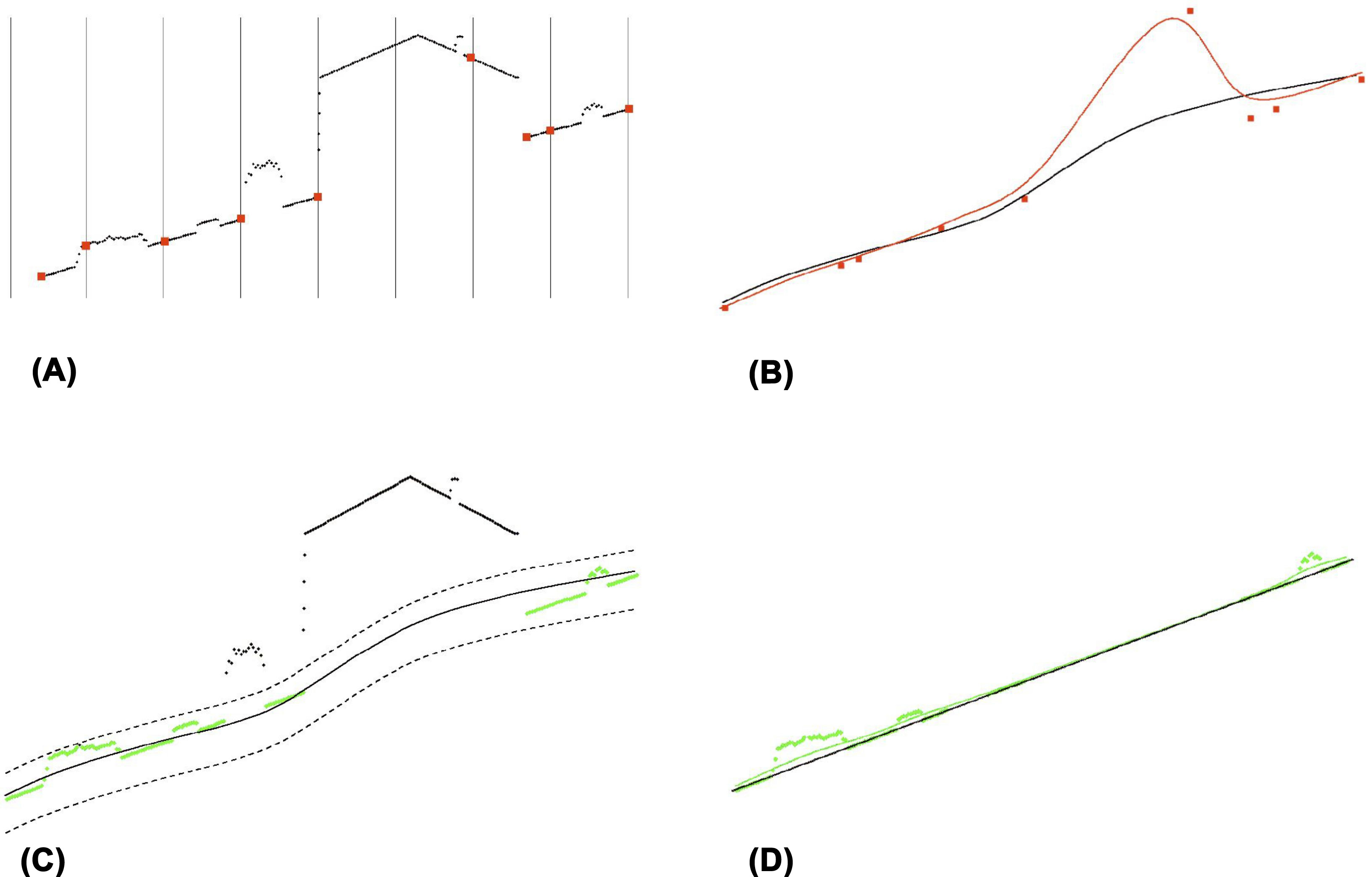
The main feature of hierarchical robust interpolation is the creation of a data pyramid representing the data at different resolution levels. Three steps are carried out at each level of the pyramid ([6]):
- thinning out of the original data according to the resolution of the current level of the data pyramid, using only points not yet classified as being off-terrain,
- generation of a DTM via robust interpolation, using the thinned-out data,
- comparison of the generated DTM with the original data. Data points outside a certain tolerance band are classified as off-terrain and are thus no longer considered in the subsequent iterations.
At the finest level, the DTM is computed from all original points classified as terrain points. Using thinned-out data, the influence of large clusters of off-terrain points (e.g., points on buildings) can be eliminated, but the resulting DTM also has a rather coarse resolution. The influence of low vegetation is eliminated using the data at a finer resolution, a process that also results in a better DTM ([6]).
DTM and DSM creation
To derive the DTM, due to the need for points at ground level, the area should preferably not be scanned during the growing season, as the presence of vegetation decreases laser impulse penetration to the ground. In contrast, for DSM derivation the growing season is more appropriate, since more laser impulses are reflected from the crowns of trees (deciduous more so than evergreen) and low vegetation. Scanning data obtained during the growing season is largely used to determine the height of vegetation cover ([39]).
The ALS data used in the present study were obtained during the growing season. As stated above, the creation of DTMs from data collected at this time of year is problematic, because laser impulses do not penetrate effectively through dense vegetation cover, resulting in absent ground points in DTM creation. Another problem associated with the processing of ALS data is the use of a filtering method and its ability to correctly classify points on the surface. Despite the availability of powerful filtering tools, around 1% of points are always incorrectly classified ([19]); these points should be reclassified either manually or by changing the filtering parameters.
Two DTMs were created, one from ALS and the other from contour data, but both at 8 m resolution. An 8 m spatial resolution was selected as the lowest spatial resolution for the DTM derived from the ALS data. A lower resolution would approach the errors of the DTM due to the low point density. The first DTM was created in SCOP++ using hierarchic robust filtering, with the EliminateBuildings step first applied, followed by ThinOut, Filter, Interpolate and SortOut. These last four steps were applied three times in order to efficiently filter off-terrain points, before the final Classify step. In the last iteration the step SortOut was missed. Incorrectly classified points were repaired in DTMaster (Inpho), which is designed for the efficient quality control of DTM and LiDAR data.
The second DTM was created from vectorised 20-m contours obtained from the WMS of the Slovakian National Forest Centre, using ArcMap 10. Also vectorised were hills, which were used to refine the DTM. The DTM itself was created using the Topo to raster tool, which is an interpolation method designed for the creation of hydrologically correct DTMs.
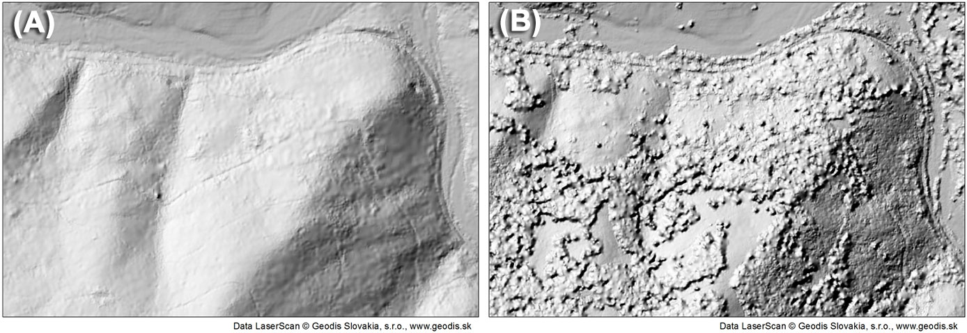
The DSM was created from ALS data using hierarchic robust filtering in SCOP++, with a resolution of 8 m. The creation of the DSM was easier than that of the DTMs, as points reflected from tree crowns were used; since the laser scanning was performed during the growing season, there were more points reflected from crowns than from the ground. In addition, it was also not necessary to filter off-terrain points. DSM hierarchic robust filtering was performed in three steps: ThinOut, Filter and Interpolate. Incorrectly classified points were repaired in DTMaster. Examples of hillshading in the first DTM and the DSM are shown in Fig. 2.
Fig. 2 - (a) DTM Hillshading; (b) DSM Hillshading.
Forest stand selection
Forest stands older than 80 years of age were selected from the FMP database. The goal was to have mostly forest stand of an exploitable age in the selection. The second selection criterion was that species representation had to be 100% in each forest stand. 43 forest stands were selected based on these two criteria, with two species, beech (Fagus sylvatica L.) and spruce (Picea abies Karst.), covering a total area of 101 ha. Stand density ranged between 0 and 1.0, although none had densities of 0.1, 0.2 and 0.3. The stand density was examined against the Forest Management Plan. Stand density is a relative measure of the length of stand occupancy by trees, as well as of the utilization of forest production; a low stand density is therefore detected after regeneration/replanting, natural disaster, etc.
Forest stand height extraction
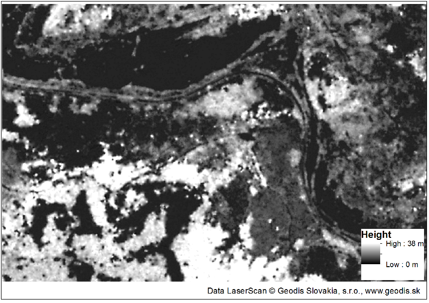
Since the DTMs represent the height of terrain and the DSM the height of objects (tree tops, buildings, etc.) above sea level, the actual height of these objects can be calculated by subtracting the former from the latter. This method, after evaluation of input data, was employed to create two normalised digital surface models (nDSMs - Fig. 3), one using the DTM created from ALS data (nDSM_L) and the other using the DTM created from contour data (nDSM_C). The cell size of both nDSMs was 8 m, with the cell value representing the height of trees in forest stands, as well as the height of buildings and other objects.
Fig. 3 - nDSM (nDSM_L) created using the ALS data-derived DTM.
For forest stands, that meet the selection criterion, zonal statistics were employed using ArcMap 10 to derive mean and maximum stand height values. The mean or maximum forest stand height was extracted using zonal statistics from the pixel values of nDSM_L and nDSM_C. Polygonal masks were used polygons to represent the borders of the selected forest stands. From these values were subtracted heights contained in the FMP database used as reference data. As forest stands varied in terms of their age and site quality, the difference between the FMP and ALS-derived heights was converted into a percentage.
A one-way analysis of variance (ANOVA) was then employed to determine the influence of tree species and stand density on tree height.
Results and discussion
Forest stand heights derived using ALS maxima were overestimated, both in nDSM_L and nDSM_C. The use of mean values largely led to an underestimation of stand height. In forest stands with the highest stand density, the forest stand height was overestimated; this occurred in three cases.
The heights of three forest stands with a density of 0.7 differed considerably in terms of the values observed in the FMP database and those derived via ALS; these differences were 97, 87 and 77% for nDSM_L and 84, 107 and 65% for nDSM_C. Consultation of orthoimages revealed these discrepancies to be a result of recent tree felling, and thus these three stands were excluded from further analysis.
The influence of tree species on ALS-derived stand height was expected to be statistically significant in all cases. However, such significance was only observed after using the mean for forest stand height extracted from both nDSMs: nDSM_L and nDSM_C. The reason for the lack of statistical significance when maxima were employed is unknown. Tab. 1 shows that stand heights derived from ALS maxima were nearer to FMP values for beech than for spruce, whereas Tab. 2 shows better results for spruce than for beech were obtained when mean height values were used. One possible explanation for this is that beech crowns are more spherical and those of spruce cone-like; as a result, more points in the point cloud reflected from such spheres are closer to the top of the crown (i.e., max. height).
Tab. 1 - Overview of statistical characteristics for tree species - FMP-max (in %).
| Tree species | Arithmetic mean | Standard deviation | ||
|---|---|---|---|---|
| ALS FMP-max |
Contours FMP -max |
ALS FMP -max |
Contours FMP -max |
|
| Beech | -16.3 | -13.3 | 20.1 | 23.2 |
| Spruce | -19.6 | -31.3 | 13.8 | 19.9 |
| Total | -17.2 | -18.3 | 18.5 | 23.6 |
Tab. 2 - Overview of statistical characteristics for tree species - FMP-mean (in %).
| Tree species | Arithmetic mean | Standard deviation | ||
|---|---|---|---|---|
| ALS FMP-mean |
Contours FMP - mean |
ALS FMP - mean |
Contours FMP - mean |
|
| Beech | 50.1 | 54.5 | 35.0 | 42.3 |
| Spruce | 19.0 | 11.7 | 17.2 | 12.7 |
| Total | 41.5 | 42.7 | 33.9 | 41.3 |
As shown in Tab. 4, the influence of stand density was statistically significant when mean was used for forest stand height extraction from both nDSMs; nDSM_L and nDSM_C. Although stand heights were generally underestimated, the heights of stands of density 1.0 were overestimated in nDSM_L and those of density 0.9 and 1.0 overestimated in nDSM_C. Tab. 4 also shows a significant difference (underestimation) between FMP and ALS-derived mean heights for low density stands (0.0 and 0.4), with values of 77 and 45%, respectively, for nDSM_L, and 81 and 37%, respectively, for nDSM_C. These discrepancies were likely caused by the reflection of laser impulses from suppressed trees, low vegetation and the ground surface. For stands of density 0.6 and higher, stand heights were relatively well described using mean values both in nDSM_L and nDSM_C.
Tab. 4 - Overview of statistical characteristics for stand density - FMP-mean (in %).
| Stand density | Arithmetic mean | Standard deviation | ||
|---|---|---|---|---|
| ALS FMP-mean |
Contours FMP - mean |
ALS FMP - mean |
Contours FMP - mean |
|
| 0.0 | 76.9 | 80.6 | 15.1 | 26.3 |
| 0.4 | 45.3 | 37.1 | 35.1 | 37.3 |
| 0.5 | 25.3 | 28.1 | 14.1 | 62.9 |
| 0.6 | 12.6 | 22.7 | 10.5 | 14.2 |
| 0.7 | 17.2 | 16.6 | 17.4 | 12.4 |
| 0.8 | 4.1 | 6.4 | 0.1 | 3.4 |
| 0.9 | 11.5 | -2.3 | 12.6 | 6.4 |
| 1.0 | -8.5 | -3.6 | - | - |
| Total | 41.5 | 42.7 | 33.9 | 41.3 |
The use of maxima values resulted in fairly good estimation of stand height for stands of low density, in both nDSM_L and nDSM_C. For stands of density 0.0, overestimation was under 8%, whereas the results for those of density 0.4 were comparable with those of higher densities (Tab. 3).
Tab. 3 - Overview of statistical characteristics for stand density - FMP-max (in %).
| Stand density | Arithmetic mean | Standard deviation | ||
|---|---|---|---|---|
| ALS FMP-max |
Contours FMP -max |
ALS FMP -max |
Contours FMP -max |
|
| 0.0 | -6.9 | -7.4 | 20.2 | 20.7 |
| 0.4 | -22.3 | -38.2 | 7.6 | 7.6 |
| 0.5 | -32.6 | -28.2 | 22.9 | 35.6 |
| 0.6 | -26.1 | -2.6 | 2.9 | 18.8 |
| 0.7 | -20.4 | -21.9 | 14.5 | 23.8 |
| 0.8 | -24.5 | -34.9 | 1.3 | 5.8 |
| 0.9 | -21.5 | -39.4 | 9.5 | 6.6 |
| 1.0 | -32.4 | -26.2 | - | - |
| Total | -17.2 | -18.3 | 18.5 | 23.6 |
The transmission of laser impulses through the canopy is not so effective in forest stands of high density. DTMs which are unable to record the terrain under forest stands will clearly have a negative influence on stand height derivation; this effect is particularly evident in the modelling of stands with densities of 0.9 and 1.0. The determination of forest stand height using the DTM created from low point density ALS data was presented in work by Smreček ([35]). The DTM created from contour lines was able to describe such terrain more accurately than that created using ALS data (Tab. 4).
The results achieved in the present study were less accurate in comparison to those achieved by other authors. The most likely reason for this is the low density of points, particularly under trees, obtained for DTM creation. Wezyk et al. ([40]) used two different tree crown surfaces, derived in the Fusion software program, to determine tree height. The first crown surface was subjected to arithmetic average and smoothing filters, while maximum and minimum values were neglected. In this case, actual measured tree heights were underestimated by about 0.9 m, with a standard deviation of 1.77. Application of the second type of crown surface included the use of maxima and minima, resulting in an underestimation of only 0.12 m, with a standard deviation of 1.81. Heurich ([14]) compared the characteristics of 0.1- 0.25 ha beech and spruce stands in the Bavarian National Park. The mean deviation between ALS-derived height and terrain measurement was -0.54 m, with the difference lower (-0.43 m) for deciduous trees and higher (-0.63 m) for coniferous trees. In their examination of spruce stands, Naesset & Økland ([26]) achieved a standard deviation of tree height determination of 0.49 m, representing 7.6% of tree height. Holmgren et al. ([17]) used linear regression functions to predict basal-area-weighted mean tree height, achieving a Root Mean Square Error (RMSE) of 1.45-1.56 m, corresponding to 10-11% of mean height. Many other authors have also found that the employment of ALS typically leads to an underestimation of tree height due to the fact that laser impulses are not reflected from the majority of tree terminals ([11], [14], [40]). However, the methods used in some other studies resulted in height overestimation. For example, Lim et al. ([24]) experienced a differential of 77%, whereas Farid et al. ([13]) overestimated the height of young cottonwood (Populus fremontii S. Watson) and mesquite (Prosopis velutina Woot.), although the latter authors believed their discrepancy in results to be caused by the reflection of laser impulses from nearby higher trees.
Conclusion
Despite the steady development of ALS which took place during the 1970s and 1980s, the technique remains limited in that elevation data can only be acquired along a single line (i.e., the flight path). If a large area of terrain is to be covered, an accordingly large number of flights must be flown in order to provide complete coverage ([32]). One of the first successful applications of laser scanning took place in the field of water depth detection, with water depth calculated as the difference between the time of first (water surface) and second (water body bed) reflections ([23]). Suitable scanning mechanisms were devised during the early 1990s and the global positioning system (GPS) constellation was completed at around the same time; with high performance IMUs also commercially available by the mid-1990s, integrated GPS/IMU georeferencing systems were thus able to deliver airborne platform position and altitude data down to a scale of 4-7 cm ([32]). ALS has developed extremely rapidly and is now in widespread use, with many authors exploring its potential for use in forestry ([27], [1], [41]). A chronology of such forestry-focused scientific research can be found in Hyyppä et al. ([18]).
A variety of methods are available with which to determine stand/tree height in intensive forest management, the precision and efficiency of which are generally well known. The comparative advantage of ALS is the possibility for high automation and of making rapid measurement of time-delay data; the use of such models to derive forest stand/tree parameters should guarantee both precision of results and the avoidance of user error. The main aim of the present paper was to demonstrate the potential for using ALS data of low point density (1 point per 3m2). Although the DTM created from these data, particularly those points under canopy cover, was of poor quality, such obstacles can potentially be overcome by the creation of a DTM using additional contour data. The DSM derived from these low point density data was also not of high quality, due to the fact that the tops of tree crowns were less likely to be hit by laser impulses. The raster resolution of both DTMs and the DSM was 8 m, which was the lowest spatial resolution possible for DTM creation from the ALS data without errors. The height of selected forest stands, older than 80 years of age, was determined using mean and maxima functions, with these values then compared with those contained in the current FMP. The results of this comparison revealed that only the use of the mean function was statistically significant, with the ALS-derived heights of stands with density greater than 0.7 similar to FMP values. In contrast, the use of the maxima function is recommended only for forests with low stand density, such as those in which seed trees are employed. The forest stand height obtained using this method with data with low point density has potential for large differences between some observed and modelled values. Thus, it is important to be aware of this when using this obtained forest stand height to obtain other forest stand parameters, because of error accumulation in the calculation. There is the possibility to improve the input data for the calculation of other forest stand characteristics, by using forest inventory data and statistical models ([3], [29], [16], [10]). Although some individual results of the present study are similar to those of other authors ([14], [40]), most are relatively poor.
As stated previously, low point density data should be carefully used for other forest stand parameter derivation. However, the cost of low point density data is less than that of high density data, and as such the former can therefore be used by state agencies or other organisations for forest management practices such as felling control, measurement of disaster area and the detection of gross mistakes in FMP data. Big differences between the forest stand height derived from the ALS data and the height obtained from the FMP were identified in three forest stands in which tree felling was done. The differences were from 77% to 97% by height extracted from nDSM_L and from 65% to 107% by height extracted from nDSM_C. The tree felling was verified on the orthoimages. DTMs employed in forestry must be of good quality, while only DSMs should be created from low point density ALS data. In addition, different respective approaches should be employed for low and high density stands, because, as shown in the present study, no single method was able to obtain good results for all stand densities.
Acknowledgments
This publication is the result of the implementation of the project: Centre of Excellence “Decision support in forest and country”, ITMS: 26220120069, supported by the Research & Development Operational Programme funded by the ERDF. The author would also like to thank Geodis Slovakia s.r.o. for providing the ALS data used in this study.
Box 1 - List of Abbreviations
The following abbreviations are used thoughout the text:
- ALS - Airborne laser scanning
- LiDAR - Light Detection and Ranging
- RADAR - Ratio Detection and Ranging
- DTM - Digital terrain model
- DSM - Digital surface model
- nDSM - Normalised digital surface model
- nDSM_L - DTM created from ALS data was used for nDSM creation
- nDSM_C - DTM created from contour data was used for nDSM creation
- FMP - Forest management plan
- WMP - Web Map Service
- FOV - Field of view
- GPS - Global positioning system
- IMU - Inertial measurement unit
References
Gscholar
Gscholar
Gscholar
Gscholar
Gscholar
Gscholar
Gscholar
Gscholar
Gscholar
Gscholar
Gscholar
Gscholar
Gscholar
Gscholar
Gscholar
Gscholar
Gscholar
Gscholar
Gscholar
Gscholar
Gscholar
Authors’ Info
Authors’ Affiliation
Department of Forest Management and Geodesy, Technical University in Zvolen, T. G. Masaryka 24, 960 53 Zvolen (Slovakia)
The Institute of Foreign Languages, Technical University in Zvolen, T. G. Masaryka 24, 960 53 Zvolen (Slovakia)
Corresponding author
Paper Info
Citation
Smreček R, Danihelová Z (2013). Forest stand height determination from low point density airborne laser scanning data in Roznava Forest enterprise zone (Slovakia). iForest 6: 48-54. - doi: 10.3832/ifor0767-006
Academic Editor
Marco Borghetti
Paper history
Received: Sep 07, 2012
Accepted: Dec 05, 2012
First online: Jan 21, 2013
Publication Date: Feb 05, 2013
Publication Time: 1.57 months
Copyright Information
© SISEF - The Italian Society of Silviculture and Forest Ecology 2013
Open Access
This article is distributed under the terms of the Creative Commons Attribution-Non Commercial 4.0 International (https://creativecommons.org/licenses/by-nc/4.0/), which permits unrestricted use, distribution, and reproduction in any medium, provided you give appropriate credit to the original author(s) and the source, provide a link to the Creative Commons license, and indicate if changes were made.

Web Metrics
Breakdown by View Type
Article Usage
Total Article Views: 59471
(from publication date up to now)
Breakdown by View Type
HTML Page Views: 49359
Abstract Page Views: 4004
PDF Downloads: 4422
Citation/Reference Downloads: 32
XML Downloads: 1654
Web Metrics
Days since publication: 4922
Overall contacts: 59471
Avg. contacts per week: 84.58
Article Citations
Article citations are based on data periodically collected from the Clarivate Web of Science web site
(last update: Mar 2025)
Total number of cites (since 2013): 16
Average cites per year: 1.23
Publication Metrics
by Dimensions ©
Articles citing this article
List of the papers citing this article based on CrossRef Cited-by.
Related Contents
iForest Similar Articles
Research Articles
Three-dimensional forest stand height map production utilizing airborne laser scanning dense point clouds and precise quality evaluation
vol. 10, pp. 491-497 (online: 12 April 2017)
Research Articles
Determining basic forest stand characteristics using airborne laser scanning in mixed forest stands of Central Europe
vol. 11, pp. 181-188 (online: 19 February 2018)
Research Articles
Integrating area-based and individual tree detection approaches for estimating tree volume in plantation inventory using aerial image and airborne laser scanning data
vol. 10, pp. 296-302 (online: 15 December 2016)
Research Articles
Are we ready for a National Forest Information System? State of the art of forest maps and airborne laser scanning data availability in Italy
vol. 14, pp. 144-154 (online: 23 March 2021)
Research Articles
Integration of tree allometry rules to treetops detection and tree crowns delineation using airborne lidar data
vol. 10, pp. 459-467 (online: 04 April 2017)
Research Articles
Comparing image-based point clouds and airborne laser scanning data for estimating forest heights
vol. 10, pp. 273-280 (online: 23 February 2017)
Research Articles
Optimizing line-plot size for personal laser scanning: modeling distance-dependent tree detection probability along transects
vol. 17, pp. 269-276 (online: 07 September 2024)
Research Articles
Prediction of stem diameter and biomass at individual tree crown level with advanced machine learning techniques
vol. 12, pp. 323-329 (online: 14 June 2019)
Research Articles
Use of terrestrial laser scanning to evaluate the spatial distribution of soil disturbance by skidding operations
vol. 8, pp. 386-393 (online: 08 October 2014)
Research Articles
Identification and characterization of gaps and roads in the Amazon rainforest with LiDAR data
vol. 17, pp. 229-235 (online: 03 August 2024)
iForest Database Search
Search By Author
Search By Keyword
Google Scholar Search
Citing Articles
Search By Author
Search By Keywords
PubMed Search
Search By Author
Search By Keyword