Estimation of forest biomass components using airborne LiDAR and multispectral sensors
iForest - Biogeosciences and Forestry, Volume 12, Issue 2, Pages 207-213 (2019)
doi: https://doi.org/10.3832/ifor2735-012
Published: Apr 25, 2019 - Copyright © 2019 SISEF
Research Articles
Abstract
In order to consider forest biomass as a real alternative for energy production, it is critical to obtain accurate estimates of its availability using non-destructive sampling methods. In this study, we estimate the biomass available in a Scots pine-dominated forest (Pinus sylvestris L.) located in Spain. The biomass estimates were obtained using LiDAR data combined with a multispectral camera and allometric equations. The method used to fuse the data was based on back projection, which assures a perfect match between both datasets. The results present estimates for each of the seven different biomass components: above ground, below ground, log, needles, and large, medium and small branches. The accuracy of the models varied between R2 values of 0.46 and 0.67 with RMSE% ranging from 15.72% to 35.43% with all component estimates below 20%, except for the model estimating biomass of big branches. The models in this study are suitable for the estimation of biomass and demonstrate that computation is possible at a fine scale for the different biomass components. These remote sensing methods are sufficiently accurate to develop biomass resource cartography for multiple energy uses.
Keywords
Biomass Components, Forest Inventory, Airborne Laser Scanning, Multispectral Imagery, Data Fusion, Nearest Neighbor
Introduction
Forest biomass is a substantial source of renewable energy, and it is becoming increasingly important for environmental and economic reasons ([39]). Studies have addressed various aspects of the use of forest residue biomass for energy production and the associated carbon emissions and sequestration ([15], [1]). Recent studies have shown that European Union countries underuse their current potential forest biomass production, and those resources are unevenly harvested across Europe ([46]). The use of forest biomass requires a higher mobilization of existing resources, using different forest components obtained from efficient and sustainable management ([39], [14]). These forest components (branches, treetops, needles and even stumps and roots) are generated through forest management, and they are not usually removed from the stand because of their small diameters.
Many forest inventories currently focus mainly on timber volume for forest industries and they usually lack the quality characteristics demanded by regional managers and renewable biomass energy industry ([37], [10], [13]). Some of those characteristics are the stock of detailed tree biomass components and the spatial location of these resources at finer scales ([27], [23]). In this sense, the contributions of remote sensing estimates are becoming a valuable tool ([15], [1]) to produce accurate and cost-competitive estimates at the landscape level ([48]). However, there are some limitations for certain remote sensing techniques, such as satellite-borne optical sensors or synthetic aperture radar, that have shown signal saturation in forest environments with very high biomass density ([7]). The use of LiDAR sensors on-board airplanes, known as airborne laser scanning, has proved to be the best option for biomass accounting, applied separately or in combination with other active or passive sensors ([4], [48]). Previous studies have shown the reliability of LiDAR to obtain estimates of above-ground biomass ([33]), below-ground biomass ([30], [19]), and of other biomass components ([37], [10], [13]). Additional studies have also investigated techniques for fusion of images from airborne or satellite-borne multispectral (MS) sensors for the purpose of biomass assessment ([35]).
Forest inventories lack information on tree biomass components and the precise spatial location of these resources at finer scales ([12]). Current methods of spatial biomass assessment based on national forest inventories present limitations such as the lack of accuracy for efficient spatial planning, among others ([32]). Many predictions of forest-based biomass have therefore been restricted to a regional scale, or have been spatially interpolated ([20]). Furthermore, thinning and other partial treatments are widely used to reduce fire risk, remove non-native and invasive species, and restore forests to historic reference conditions, often at high net cost ([1]). In most cases, this forest waste generated by thinning and clearing is not used for any purpose, because it is not included in current inventories.
In the present study, we introduce a novel framework for predicting biomass based on the combination of airborne LiDAR and multispectral cameras, using advanced techniques of sensor fusion and non-parametric imputation ([5], [6]) that minimize noise and loss of information.
Material and methods
Study area and field information
Fig. 1 - Study area location (red rectangular frame) and field plot distribution (black dots).
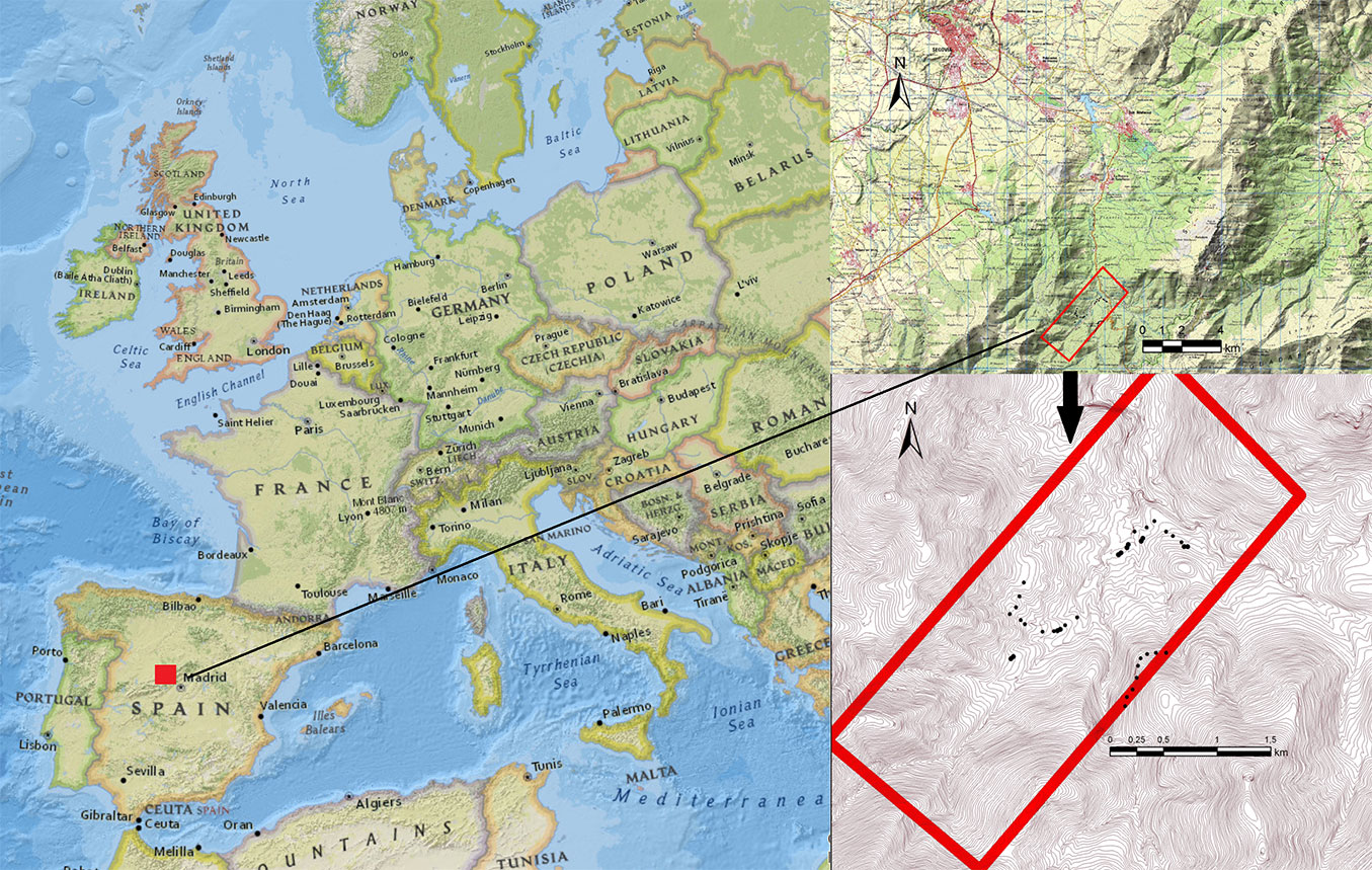
The studied area (Fig. 1) was a Scots pine-dominated (Pinus sylvestris L.) forest in Valsaín (Spain; approx. coordinates: 41° 44′ N, 04° 39′ W; elevation 1300-1500 m a.s.l.). The ground data included 37 plots; each plot entailed two concentric circles with radii of 10 m and 20 m, respectively ([43]). In the inner circle, all trees were measured, including seedlings and saplings, whereas in the outer circle only trees with diameter at breast height (dbh, cm) over 10 cm were measured. Corroborating within-plot homogeneity in the field, information sampled within the inner plot was expanded to the outer plot ([43]). Tree top height (h, m) was determined with a Vertex III Hypsometer (Haglof, Sweden). Plot centers were staked out using a HiPer-Pro® (Topcon, California) receiver set at 1-2 m above the ground for differentially-corrected global navigation satellite systems (GNSS) positioning ([42]). Mean stand density (± standard deviation) of the study area was 732.3 ± 559.2 stems ha-1, mean basal area was 41.8 ± 11.2 m2 ha-1 and mean standing volume was 390.7 ± 258.6 m3 ha-1. Locally-adjusted tree allometry specific for P. sylvestris was employed to derive the dry-weight biomass components ([27]). Equations were used for above-ground biomass (agb, kg), root biomass (below-ground biomass: bgb, kg), log biomass (lb, kg), needle biomass (nb, kg), and branch biomass (bb) with diameter Ø > 7 cm (big-branch biomass: bbb, kg), 2 > Ø > 7 cm (medium-branch biomass: mbb, kg) and Ø < 2 cm (small-branch biomass: sbb, kg), following (eqn. 1-eqn. 7):
The forest stand attributes and characteristics were calculated by aggregating the tree-level biomass estimates (in lower-case letters, kg) into per-hectare totals at the plot-level (capital letters, Mg ha-1). The biomass components were organized into three hierarchical groups: the first group showed components of total biomass, above-ground biomass (AGB, Mg ha-1) and below-ground biomass (BGB, Mg ha-1), obtained as aggregations of the values calculated with eqn. 1 and eqn. 2, respectively. The second group disaggregated AGB into several components: log biomass (LB, Mg ha-1), needle biomass (NB, Mg ha-1) and branch biomass (BB, Mg ha-1). LB and NB were obtained using eqn. 3 and eqn. 4, respectively, whereas BB was calculated as aggregation of eqn. 5, eqn. 6, and eqn. 7 separated into components, namely: big (bBB, Mg ha-1), medium (mBB, Mg ha-1) and small (sBB, Mg ha-1) branch biomass. Biomass components of the study area, derived from the sample plots, are given in Tab. 1.
Tab. 1 - Summary of field plot reference data (Mean; Standard deviation, SD; Maximum, Max; Minimum, Min; Coefficient of Variation, CV) of the different observed biomass components.
| Components in Mg ha-1 | Mean | SD | Max | Min | CV |
|---|---|---|---|---|---|
| Above-ground biomass (AGB) | 211.313 | 58.140 | 318.798 | 106.474 | 0.275 |
| Below-ground biomass (BGB) | 61.140 | 18.426 | 94.528 | 27.623 | 0.301 |
| Log biomass (LB) | 175.830 | 54.707 | 274.803 | 76.653 | 0.311 |
| Needle biomass (NB) | 10.544 | 2.885 | 17.212 | 4.615 | 0.274 |
| Big-branch biomass (bBB) | 8.959 | 4.561 | 19.761 | 1.416 | 0.509 |
| Medium-branch biomass (mBB) | 18.763 | 4.630 | 27.878 | 9.286 | 0.247 |
| Small-branch biomass (sBB) | 13.977 | 3.824 | 22.816 | 6.118 | 0.274 |
Remote sensing datasets and back-projecting sensor fusion
Active LiDAR and passive MS sensors were installed together on a gyro-stabilized platform on-board a 404-Titan™ (Cessna, Kansas, USA) with double photogrammetric window, in-flight GNSS and inertial navigation systems (INS). These provided the position and attitude of each sensor, which were used as external orientation in the sensor fusion procedure ([41]) as described below. The LiDAR sensor consisted of an airborne laser scanner ALS50-II® (Leica Geosystems, Switzerland) operating at a pulse frequency of 55 kHz. A maximum of four separate discrete returns were obtained from an approximate pulse footprint diameter of 0.5 m at nadir ([3]). The flight took an approximate height of 1500 m and ground speed of 72 m s-1. These flight parameters yielded a nominal average pulse density of 1.15 pulses m-2 ([3]). An approximate total area of 800 ha was covered by four scan lines with a swath width of 665 m and a 40% side lap. Returns were classified as ground using a lowest elevation of 2 m and threshold angle of 12-75° in Terrascan® (Terrasolid, Finland). Ground returns were interpolated into a digital terrain model (DTM) at a spatial resolution of 1 m. Based on ground surveying quality control, its precision was calculated to be approximately 15 cm. The DTM values were subtracted from each individual return, obtaining their heights above ground (H, m).
The MS sensor consisted of a digital mapping camera (DMC®, Zeiss-Intergraph, Germany) system composed of four charge-coupled device (CCD) heads preceded by filters providing selective sensitivity for red, green, blue and near-infrared (NIR). These were the original bands of narrower spectral resolution and coarser spatial resolution (in comparison with the radiometric information registered by the panchromatic lens system) which was dismissed from this study in order to maintain the integrity of the irradiance recorded for the narrow bands. Digital numbers obtained with a 12-bit radiometric resolution from the spectral bands for red and NIR were employed to obtain (non-orthorectified) images containing NDVI values calculated at pixel-level.
These images had an approximate ground sampling distance of 60 cm, as can be deduced from the given flight height and the focal length of f = 30 mm of these MS heads. The lenses of the matricial array frame of the described DMC system, however, direct the light to a matrix of CCD sensors with a central projection. Due to this perspective, equal segments within the NDVI image represent different distances on the ground, depending whether they are at nadir or close to the edge of the image. As an airborne sensor, while the low flying altitude yielded high spatial resolutions, it also presented the shortcoming that anisotropy and within-picture scale differences according to nadir angles are larger than when using a satellite-borne sensor. For these reasons, we chose to fuse sensor data using a projection procedure, since this assured the correspondence between the H and NDVI information ([41]). The procedure consisted of projecting each first return from the LiDAR dataset into the most nadiral NDVI image available, retrieving the NDVI value of the pixel at that position, which effectively resulted in an NDVI-colored LiDAR point cloud. In order to model the central perspective of the MS sensor and render the positions of LiDAR returns on the ground onto the location of the CCD frame at the time of exposure, the three-dimensional geo-coordinates of each LiDAR return (X, Y, Z; m) were projected into two-dimensional photo-coordinates (Xph, Yph; mm) according to the collinearity equations (eqn. 8, eqn. 9):
where the center of the NDVI image was given by the principal point (Xpp, Ypp; mm) obtained, and the position of the plane at the time of exposure (Xo, Yo, Zo; m) was given by the GNSS position of the platform obtained in-flight. Likewise, the INS provided information on the attitude of the CCD frame axes with respect to the coordinate system used as the plane’s roll, pitch and yaw (ω, φ, κ; rad), i.e., rotation angles around along-track, across-track and vertical axes from the sensor’s platform, respectively. These angle parameters were used to define the rotation matrix M3G3 = (m11, …, m33) that was applied to eqn. 8 and eqn. 9. The resulting root mean square error in co-registration of the LIDAR-MS fusion product was 0.54 m, therefore mainly dependent on the spatial resolution of the MS image ([41]).
Predictor computation and most similar neighbor imputation
The colored ALS returns backscattered from the measured field plots were extracted, in order to calculate area-based predictor variables from them ([22]) using FUSION software (USDA Forest Service - [24]). In addition to the traditional H metrics describing the distribution of ALS heights ([29], [21]), we also calculated descriptors for the distribution of NDVI values, therefore obtaining NDVI metrics (henceforth indicated as either Hxxx or NDVI.xxx, where xxx refers to each given metric). All of these metrics were used as a matrix of predictors including both H and NDVI metrics (XH+NDVI - [22]) for the MSN (Most Similar Neighbor) estimation ([25]) of the biomass components Y = (AGB, BGB, LB, NB, BB, bBB, mBB, sBB). These were done using the package “yaImpute” ([8]) for k-NN imputation in the R statistical environment ([36]), which has already been demonstrated to be useful in predicting forest variables using LiDAR data ([6]) and multispectral data ([28]). The feature space X was modified into projections obtained from a canonical correlation analysis (CCA), which compressed the original multidimensionality into a few components which maximized cov(X,Y). Hence, these components were linear combinations of the response (U) and predictors (V) (eqn. 10, eqn. 11):
where α and γ were the canonical coefficients of Y and X, respectively. Twenty combinations of both H and NDVI metrics were selected based on the CCA results ([22]) and hypothesis tests ([40]), eliminating those that induced collinearity and redundancy and keeping those providing higher proportions of explained variance. The MSN procedure then computed a matrix of distances among all the field plots in the modified feature space V. Setting a value of k = 3 neighbors, on the basis of previous experience ([44]), the nearest neighbors were searched among the remaining of the plots under the criterion of the shortest distances in V. MSN estimation for each plot was finally done by imputing an inverse-distance weighted average of the values of Y for its most similar neighbors.
Accuracy assessment
Estimates of biomass components were evaluated by means of leave-one-out cross-validation, so that each field plot (i) was eliminated from the dataset prior to model training for its own prediction. A predicted value of Y (prei) was then obtained for that plot, which was compared to the value measured in the field (observed, obsi). We evaluated the estimation of forest biomass components by means of the bias and precision of the mean of predictions, respectively considered as the absolute and relative (in relation to the empirical mean, obs) difference of means (bias) and root mean squared differences (RMSD - eqn. 12, eqn. 13, eqn. 14, eqn. 15):
Also, with the aim of determining an indicator of the degree of agreement between the cross-validated predictions and the observed values, we calculated their coefficient of determination (R2) and index of agreement (d) as (eqn. 16, eqn. 17):
The coefficient of determination was reported since it is the most customarily employed statistic, although the index of agreement has been suggested as a more correct means to compare predicted vs. observed values ([47]). The cross-validated predictions also underwent hypothesis tests based on their regression to the observed values ([34]) and a measure of over-fitting ([40]), so that whenever these tests failed the model was rejected and the initial selection of predictors was further constrained ([40]).
Results
Above- and below-ground biomass
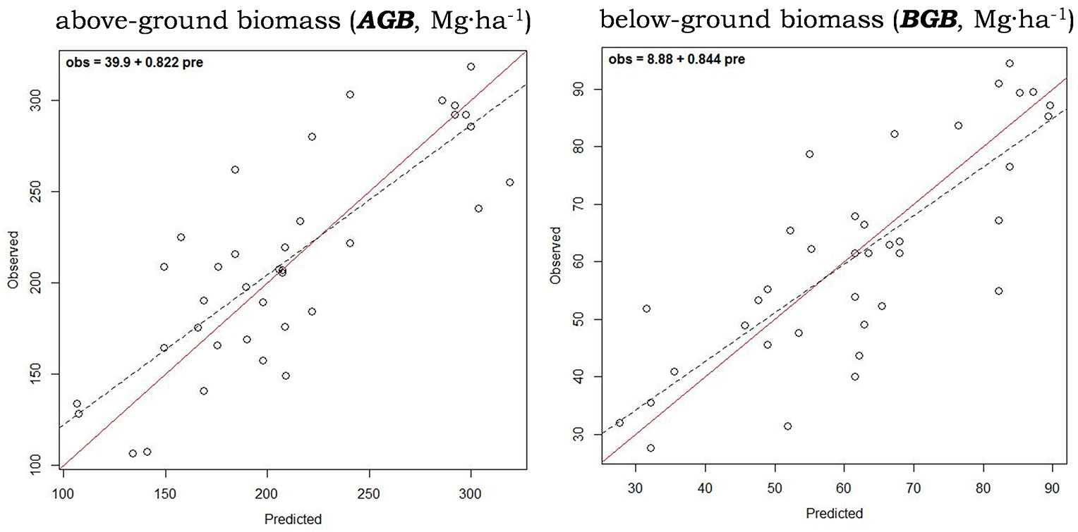
The hypothesis tests applied to the 1:1 fit of observed vs. predicted plots corresponding to above and below-ground biomass models were successful, obtaining unbiased predictions (obs = 39.9 + 0.822 · pre, and: obs = 8.88 + 0.844 · pre, respectively - Fig. 2). The relative precision of the AGB and BGB estimates (RMSD%) ranged from 16.72% to 18.44% respectively and the absolute precision of the estimates (RMSD) from 35.340 Mg ha-1 for above-ground biomass to 11.276 Mg ha-1 for below-ground biomass (Tab. 2). They reached an index of agreement (d) of 81.9% and 81.1% between observed and predicted, with 64.3% and 62.9% of explained variance (R2), respectively (Tab. 2).
Fig. 2 - Observed vs. predicted (cross-validated) values of above and below-ground biomass. The solid diagonal represents the 1:1 correspondence. Dashed line is the linear regression fit for prei = α + β · obsi, expressed in the upper left corner.
Tab. 2 - Summary diagnosis (bias, Mg ha-1; percentage of bias, %; root mean square difference, RMSD, Mg ha-1; percentage of RMSD, %; coefficient of determination, R2; index of agreement, d) of most similar neighbor (MSN) predictions for above and below-ground fractions of total biomass.
| Biomass components | bias (Mg ha-1) |
bias% (%) |
RMSD (Mg ha-1) |
RMSD% (%) |
R 2 | d |
|---|---|---|---|---|---|---|
| Above-ground biomass (AGB) |
-1.247 | -2.635 | 35.34 | 16.724 | 0.643 | 0.819 |
| Below-ground biomass (BGB) |
0.803 | 1.313 | 11.276 | 18.443 | 0.629 | 0.811 |
Components of above-ground biomass
The hypothesis tests applied to the 1:1 fit of observed vs. predicted plots corresponding to models for the separate components of the AGB predicting the biomass accumulated at the log, branch and needle levels, respectively LB, BB and NB also passed successfully, showing unbiased predictions (obs = 28.5 + 0.816 · pre; obs = 2.39 + 0.759 · pre; and obs = 5.41 + 0.844 · pre, respectively - Fig. 3). These models had a RMSD% ranging between 18.21% and 19.99% (Tab. 3). They reached a d ranging from 84.3% to 72.5% between observed and predicted, with 46.2% and 66.8% of explained variance. The highest R2 values corresponded with the log biomass model and the lower with the model predicting biomass content for branches.
Fig. 3 - Observed vs. predicted (cross-validated) values for separate components of above-ground biomass: log, needle and branch biomass. The solid diagonal represents the 1:1 correspondence. Dashed line is the linear regression fit for prei = α + β · obsi, expressed in the upper left corner.

Tab. 3 - Summary diagnosis (bias, Mg ha-1; percentage of bias, %; root mean square difference, RMSD, Mg ha-1; percentage of RMSD, %; coefficient of determination, R2; index of agreement, d) of most similar neighbor (MSN) predictions for separate fractions of above-ground biomass: log, needle and branch biomass.
| Biomass components | bias (Mg ha-1) |
bias% (%) |
RMSD (Mg ha-1) |
RMSD% (%) |
R 2 | d |
|---|---|---|---|---|---|---|
| Log biomass (LB) |
4.683 | 2.664 | 32.599 | 18.54 | 0.668 | 0.843 |
| Needle biomass (NB) |
0.198 | 1.882 | 2.108 | 19.99 | 0.493 | 0.725 |
| Branch biomass (BB) |
0.654 | 1.708 | 6.967 | 18.205 | 0.462 | 0.736 |
Different-sized components of branch biomass
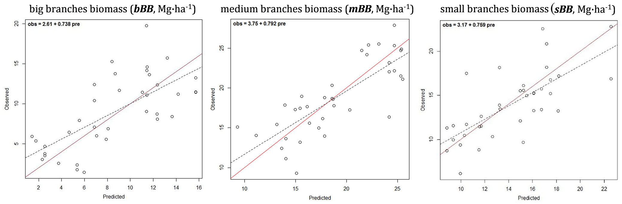
The hypothesis tests applied to the 1: 1 fit of observed vs. predicted plots corresponding to models predicting biomass for the different branch sizes (big, medium and small) also showed unbiased predictions (obs = 2.61 + 0.738 · pre; obs = 3.75 + 0.792 · pre; and obs = 3.17 + 0.759 · pre, respectively - Fig. 4). The model predicting biomass in big branches (bBB) had the biggest relative error 35.43% (Tab. 4). It is also worth to mention that in the particular case of the MSN estimation of biomass in big branches, bBB, the CCA-based preselection of variables with hypothesis test restriction showed no explanatory capacity for any of the NDVI metrics included. Regarding the other two branch size models: medium and small branches, their RMSD% ranged 15.72-19.99% and the index of agreement reached 81.4%, and the model predicting biomass for medium branches had the highest R2.
Fig. 4 - Observed vs. predicted (cross-validated) values of components of branch biomass separated by size. The solid diagonal represents the 1:1 correspondence. Dashed line is the linear regression fit for prei = α + β · obsi, expressed in the upper left corner.
Tab. 4 - Summary diagnosis (bias, Mg ha-1; percentage of bias, %; root mean square difference, RMSD, Mg ha-1; percentage of RMSD, %; coefficient of determination, R2; index of agreement, d) of most similar neighbor (MSN) predictions for branch biomass fractions separated by size. Biomass in branches with diameter > 7 cm (big branches, bBB), 2 > diameter > 7 cm (medium branches, mBB) and diameter < 2 cm (small branches, sBB).
| Biomass components | bias (Mg ha-1) |
bias% (%) |
RMSD (Mg ha-1) |
RMSD% (%) |
R 2 | d |
|---|---|---|---|---|---|---|
| Big-branch biomass (bBB) |
-0.158 | -1.768 | 3.174 | 35.432 | 0.545 | 0.701 |
| Medium-branch biomass (mBB) |
0.180 | 0.958 | 2.950 | 15.721 | 0.617 | 0.814 |
| Small-branch biomass (sBB) |
0.263 | 1.882 | 2.794 | 19.988 | 0.493 | 0.725 |
Discussion
The present study assessed forest biomass components using a remote sensing technique that combines LiDAR metrics with NDVI computed from a multispectral camera, complementing previous research on the estimation of forest biomass through the fusion of active and passive sensors ([9]). The biomass assessment was carried out separately for the different forest biomass components in order to provide detailed information useful for bioenergy production purposes. The results were generated using allometric equations developed for the region and targeted at different species ([27]).
The added value of the results presented in this study lies in the improvements achieved in comparison to previous studies using similar or alternative methodologies. Previous biomass studies using airborne LiDAR have used indirect calculations by extracting the forest variable values from LiDAR data and then using them as an input in the biomass allometric equations ([18]). Other studies have calculated biomass directly from LiDAR data but focusing only on above ground biomass ([30], [10]) or on some of the components to estimate their contribution to carbon stocks ([26]), but not for the whole tree with roots included. There is also an added value for the combination of LiDAR data with multispectral sensors ([39]), and in particular for the data fusion improvements implemented in this study ([41]), and the feasibility of the estimation method for the assessment of forest variables ([25], [31]).
The assessment of separate components of above-ground biomass provides forest managers with greater flexibility in decision-making, since not all the components are considered for the same purpose, depending on wood quality and market prices ([38]). Logs are usually the main product, and other parts like small branches and treetops are left on the ground for environmental reasons, but they can also be used for energy purposes, providing an added value ([2]). The estimation of all the above ground biomass components is therefore fundamental to correctly assess the energy potential of a certain area or region ([45]). On the other hand, foliage should not be included as biomass for energy, due to the ecologic role it plays in the nutrient cycle ([39]). The results obtained in this study showed that these remote sensing methods have great potential for reliably estimating below-ground biomass, and not only above-ground biomass. Their estimation is therefore more practical for ecological purposes ([26]). Though the accuracy of our models was not as high as in other studies ([10]), we can still conclude that LiDAR is a suitable tool to assess branch biomass, and branch biomass is better assessed from the air than from field measurements ([13]). In the case of below-ground biomass components, these presented a higher predictive power taking into account that this component is retrieved by surrogating relations, and there is no direct relation with LiDAR returns or with the multispectral camera.
Previous studies have included treetop estimates as a part of the big-branch biomass estimates ([16]). In this study, it was not possible to consider this fact as a separate component due to the lack of available allometric equations considering tree tops as a separate part of the branches or stem. Treetops are a common logging waste, often used for energy purposes, and although they represent a small percentage of the trees biomass, they can result in an average annual potential ca. 0.27 million m3 of biomass for energy. It would therefore be interesting to devote further studies to the development of specific allometric equations for this biomass component in particular. Although the use of allometric equations as reference values present limitations, they are considered the most available source for ground data, since it would be unfeasible to apply destructive sampling in every separate study ([13]). It would also be interesting to apply the same methodology in other forest stands with different characteristics (species and ages) to develop a sensitive analysis observing how the biomass estimation changes under other conditions.
Estimates of available biomass resources should be accurate, especially when related to management decisions and planning of biomass supply (for new or existing energy plants), and previous studies have recommended a threshold of 20% requirement for RMSE% when estimating biomass from LiDAR ([48]). Our results fulfill this recommended threshold in all the components except for big-branch biomass (bBB). A general comparison of our results with similar studies ([10], [11]) demonstrates higher accuracy in our approach: lower error, better R2 and better index of agreement. These improvements are related to the combined use of LiDAR and multispectral sensors ([22]) and the perfect match between both datasets achieved by the back-projecting data fusion method ([41]).
Considering these sensor-fusion techniques (combination of airborne LiDAR and multispectral camera) that minimize noise and loss of information, we recommend that future forest inventories include forest biomass mapping for renewable biomass energy ([14]). Further research could use this type of cartography to optimize transportation, which is the most expensive operational phase in this process ([17]), and evaluate derived trade-offs accounting for transportation costs as well ([12]).
Conclusions
From our results, we can conclude that the combination of LiDAR and NDVI from a multispectral camera is a valid approach to estimate the different forest biomass components. The combined use of adequate allometric equations, back-projection data fusion and Most Similar Neighbor methods provided an estimate using the latest advances in the state-of-the-art of multi-source assessment of biomass for bioenergy purposes. The methods adopted here represent a useful tool for applications of forest biomass availability and spatial distribution where more detailed information of the different components is required. It also demonstrates that computation can be done at a fine scale, for the different forest biomass components, and that it is sufficiently accurate to develop cartography for bioenergy resources management.
Acknowledgments
This work was partially supported by the Spanish Directorate General for Scientific and Technical Research under Grant CGL2013-46387-C2-2-R. We also thank the Valsain Forest Center, of the National Park Body (Spain), for their valuable help. Ruben Valbuena’s work is supported by an EU Horizon 2020 Marie Sklodowska-Curie Action entitled “Classification of forest structural types with LiDAR remote sensing applied to study tree size-density scaling theories” (LORENZLIDAR-658180).
References
CrossRef | Gscholar
CrossRef | Gscholar
Authors’ Info
Authors’ Affiliation
José Antonio Manzanera
Antonio García-Abril
Universidad Politécnica de Madrid, E.T.S.I. Montes, Research Group SILVANET, Ciudad Universitaria, 28040 Madrid (Spain)
Blas Mola-Yudego 0000-0003-0286-0170
Matti Maltamo
University of Eastern Finland, School of Forest Sciences, P.O. Box 111, FI80101, Joensuu (Finland)
University of Cambridge, Department of Plant Sciences, Forest Ecology and Conservation, Downing Street, CB2 3EA Cambridge (UK)
Bangor University, School of Natural Sciences, Thoday building, LL57 2UW Bangor (UK)
Corresponding author
Paper Info
Citation
Hernando A, Puerto L, Mola-Yudego B, Manzanera JA, García-Abril A, Maltamo M, Valbuena R (2019). Estimation of forest biomass components using airborne LiDAR and multispectral sensors. iForest 12: 207-213. - doi: 10.3832/ifor2735-012
Academic Editor
Davide Travaglini
Paper history
Received: Jan 22, 2018
Accepted: Feb 06, 2019
First online: Apr 25, 2019
Publication Date: Apr 30, 2019
Publication Time: 2.60 months
Copyright Information
© SISEF - The Italian Society of Silviculture and Forest Ecology 2019
Open Access
This article is distributed under the terms of the Creative Commons Attribution-Non Commercial 4.0 International (https://creativecommons.org/licenses/by-nc/4.0/), which permits unrestricted use, distribution, and reproduction in any medium, provided you give appropriate credit to the original author(s) and the source, provide a link to the Creative Commons license, and indicate if changes were made.

Web Metrics
Breakdown by View Type
Article Usage
Total Article Views: 51994
(from publication date up to now)
Breakdown by View Type
HTML Page Views: 39814
Abstract Page Views: 6827
PDF Downloads: 4289
Citation/Reference Downloads: 15
XML Downloads: 1049
Web Metrics
Days since publication: 2626
Overall contacts: 51994
Avg. contacts per week: 138.60
Article Citations
Article citations are based on data periodically collected from the Clarivate Web of Science web site
(last update: Mar 2025)
Total number of cites (since 2019): 16
Average cites per year: 2.29
Publication Metrics
by Dimensions ©
Articles citing this article
List of the papers citing this article based on CrossRef Cited-by.
Related Contents
iForest Similar Articles
Research Articles
Integrating area-based and individual tree detection approaches for estimating tree volume in plantation inventory using aerial image and airborne laser scanning data
vol. 10, pp. 296-302 (online: 15 December 2016)
Research Articles
Are we ready for a National Forest Information System? State of the art of forest maps and airborne laser scanning data availability in Italy
vol. 14, pp. 144-154 (online: 23 March 2021)
Technical Advances
Forest stand height determination from low point density airborne laser scanning data in Roznava Forest enterprise zone (Slovakia)
vol. 6, pp. 48-54 (online: 21 January 2013)
Research Articles
Optimizing line-plot size for personal laser scanning: modeling distance-dependent tree detection probability along transects
vol. 17, pp. 269-276 (online: 07 September 2024)
Research Articles
Three-dimensional forest stand height map production utilizing airborne laser scanning dense point clouds and precise quality evaluation
vol. 10, pp. 491-497 (online: 12 April 2017)
Research Articles
Prediction of stem diameter and biomass at individual tree crown level with advanced machine learning techniques
vol. 12, pp. 323-329 (online: 14 June 2019)
Research Articles
Determining basic forest stand characteristics using airborne laser scanning in mixed forest stands of Central Europe
vol. 11, pp. 181-188 (online: 19 February 2018)
Review Papers
Integration of forest mapping and inventory to support forest management
vol. 3, pp. 59-64 (online: 17 May 2010)
Research Articles
Integration of tree allometry rules to treetops detection and tree crowns delineation using airborne lidar data
vol. 10, pp. 459-467 (online: 04 April 2017)
Research Articles
Comparing image-based point clouds and airborne laser scanning data for estimating forest heights
vol. 10, pp. 273-280 (online: 23 February 2017)
iForest Database Search
Google Scholar Search
Citing Articles
Search By Author
Search By Keywords
PubMed Search
Search By Author
Search By Keyword


