Incorporating management history into forest growth modelling
iForest - Biogeosciences and Forestry, Volume 4, Issue 5, Pages 212-217 (2011)
doi: https://doi.org/10.3832/ifor0597-004
Published: Nov 03, 2011 - Copyright © 2011 SISEF
Research Articles
Collection/Special Issue: COST Action FP0903 (2010) - Rome (Italy)
Research, monitoring and modelling in the study of climate change and air pollution impacts on forest ecosystems
Guest Editors: E Paoletti, J-P Tuovinen, N Clarke, G Matteucci, R Matyssek, G Wieser, R Fischer, P Cudlin, N Potocic
Abstract
Mechanistic modelling is an important tool for understanding the impacts of climate change and pollutants on forest growth. One of the common practical limitations of these models is a lack of specific information regarding management activities such as thinning or harvesting, which can have a very strong influence on the accuracy of results. The use of inventory data for model parameterization and calibration is also problematic, as inventories are designed to have large volumes of data amalgamated to give accurate mean results across large areas. The precision of single point estimates is often quite low.This study uses BIOME-BGC to model forest growth on 1133 sites of the Austrian National Forest Inventory, and develops a method to estimate timber removal patterns prior to the commencement of record keeping on the sites. Recognizing the poor precision of individual point estimates in the data, we do not seek to precisely calibrate the model to the data on each point. Rather, we assume that the point-wise inventory estimates will be normally distributed around the true values. We then model each site assuming no management interventions, and compare this with inventory results. Plotting the “error” between model results and NFI data shows a strong right-skew, reflecting the modelled lack of timber removals. A Box-Cox transformation of the error plot, centred on zero, would represent an unbiased model estimate of the data, thus we can determine the historic timber removals as the difference between the original error curve and its Box-Cox transformation. Calibrating the model with this information allow us to represent forest volume with greater accuracy than would otherwise be possible.
Keywords
BIOME-BGC, Inventory, Uncertainty, Thinning, Model initialisation
Introduction
Mechanistic modelling is an increasingly popular method of tracking carbon fluxes in forest ecosystems, important for carbon balance studies, climate and pollution studies and others. Properly calibrated and validated, such models can also be used as diagnostic tools, to separate the influence of forest growth impactors such as climate change and Nitrogen deposition ([8]). Such models have however been sometimes criticised in the past for a poor representation of forest mass growth ([29], [26]). This paper presents part of a wider study that will compare aboveground biomass estimates obtained with the BIOME-BGC model ([33], [23]) with field data from the Austrian National Forest Inventory ([9]). We detail here the methodology developed to estimate forest management activities that may have occurred prior to the starting date of the available inventory data.
BIOME-BGC simulates fluxes and pools of carbon, water and nitrogen, beginning with a spin-up run of many forest growth cycles, to estimate a natural forest stand for the site without human influence ([24]). We follow this with two cycles of clear cutting to represent early industrial forest use in Central Europe, with the final start date of the present forest established in accordance with the mean forest age for each site from the NFI data. In managed forests it is likely that some biomass removals have occurred in the current forest rotation, but if these were prior to the commencement of the inventory programme then the timing and extent of those thinnings is unknown. As forest management is one of the major influences on forest carbon fluxes and pools ([30], [11], [17]), this represents a potentially serious source of uncertainty or bias in model outputs ([38]). In a recent Europe-wide comparison of forest models, Tupek et al. ([34]) did not include management in their BGC simulation, yet recognise management as a major factor.
Direct site-by-site comparisons of model outputs with inventory measurements is difficult, due to the fundamentally different approaches to scale. Models assume homogeneity at the scale of their input data ([14]), where single sites are assumed to be representative of a broader area. Inventories on the other hand are a statistical measure, designed so that a large number of results are aggregated to give a mean figure for a region or strata. Although at a broad scale the results should be comparable, individual site-by-site comparisons are likely to have little meaning. In terms of using inventory data for model initialisation and validation, this means that some liberties must be taken with the strictly mechanistic operation of biogeochemical process models, as a large component of random error in the individual plot observations must be incorporated.
National forest inventories (NFIs) contain a vast body of information, however the use of this data for research purposes has to date been limited ([18]), and few biogeochemical analyses have been applied to inventory data ([27]). This is likely due to two complications, the first to do with the data needs of complex biogeochemical models and the second with the statistical nature of forest inventories. Comprehensive inventories such as the Austrian NFI ([9]), species-specific model parameterisation ([23]) and modern spatial interpolation methods ([21]) may fulfil most of the data needs, but the uncertainty of prior management activities remains.
Comparison of biogeochemical modelling and inventory results in managed forests requires solving two simultaneous problems: the statistical uncertainty of the inventory data at the plot scale and the lack of knowledge of historical management. Our approach in this paper is to assume that the errors in a sophisticated NFI and a mature, well-tested model will both be normally distributed around zero, and thus, if assumptions of plot management history are correct, the site-by-site disagreements between the two approaches will also be normally distributed around zero.
Data and methods
The Austrian National Forest Inventory ([9]) is organized into tracts each of 4 points on a 200m square. 5600 such tracts are arranged in a square grid pattern across the country, including over areas that are not currently forested. An angle-count with a basal area factor of 4 is performed on each point, recording all trees of over 10.5cm dbh. A fixed-area plot of radius 2.60 metres is installed to record all trees of dbh between 5.0 and 10.5cm. Twenty percent of plots were measured each year, and re-measured after 5 years. Timber volumes are calculated here from measured diameters and heights using the allometric equations of Pollanschütz ([25]). Using one point from each forested tract, a total of 2224 points is obtained. We use here a subset of the database for the measurement periods 1981-85 and 1986-91, and limit the analysis to those plots with forest present in both periods, a species homogeneity of over 80 percent by basal area and less than 30 percent timber removal from the plot between the measurement periods, as our current version of BIOME-BGC has not been tested for mixed-species forests and a major removal within the increment period could confuse the results. This limits our analysis to 1133 plots.
Separate species parameterisations are available for Norway spruce (Picea abies) depending on site elevation above or below 1000m asl ([23]), but as no parameters are available for Silver fir (Abies alba) these were modelled as low elevation spruce giving a total of 386 plots (354 spruce dominated, 32 fir) in this group. Some 439 plots were high elevation spruce, 80 Pinus (67 Scots pine Pinus sylvestris and 13 Pinus nigra), 47 Larch (Larix decidua), 28 combining Oak (Quercus robur/petraea) and Ash (Fraxinus excelsior), 146 beech (Fagus sylvatica) and other broadleaves and seven stone pine (Pinus cembra).
BIOME-BGC is a mechanistic model developed to simulate the ecosystem processes of a forest stand on a daily timestep. Storages and fluxes of water, carbon and nitrogen are tracked throughout various pools in the vegetation, litter, and soil. The model has been widely applied across a range of forested ecosystems around the world, has been extensively compared with flux measurements ([32]), and was specifically parameterized and validated for major central European species by Pietsch et al. ([23]). Norway spruce in particular has been widely studied with BIOME-BGC ([4], [15], [22], [12]), giving confidence that the model can accurately represent spruce growth across a range of different circumstances. Forest management operations were included in BIOME-BGC by Cienciala & Tatarinov ([4]) and Petritsch et al. ([22]), based on prescribed management regimes.
Net primary production of the 1133 plots in our dataset is simulated using the Austrian incarnation of the DAYMET climate interpolation ([19], [7]). Species and age information is obtained from the NFI, and other inputs comprise of an interpolation of Austrian soil data ([21]), a 1 km² nationwide raster of nitrogen deposition in 1995 ([28]) and species-specific parameters determined by Pietsch et al. ([23]). BIOME-BGC operates by simulating the development of an unmanaged forest over many centuries, until a point where carbon pools are meta-stable over the course of successive mortality cycles ([24]). This is followed by two cycles of clearcutting and replanting to simulate early-industrial forest exploitation in Central Europe, and the planting date for the current stand is determined from the NFI data.
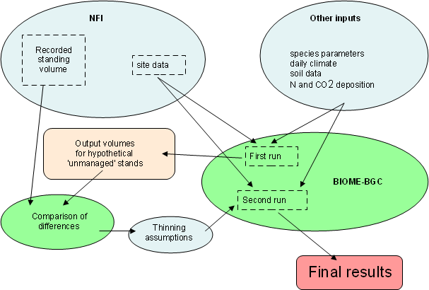
The primary output of BIOME-BGC is net primary production (NPP). Internal routines allocate this in fixed proportions to the various tree compartments, of which we are here interested in aboveground wood carbon. Without consideration of current rotation management, the model output would apply to a potential, unmanaged forest condition. In most cases this gives a biomass estimate substantially higher than the recorded data from the NFI. At the plot level the NFI data is extremely imprecise, so a four step procedure was developed to determine the appropriate removal assumptions to include in the modelling. These assumptions are then used in a second simulation of forest growth to determine final results (Fig. 1).
Fig. 1 - Schematic diagram of modelling procedure. The first run of the BIOME-BGC model is conducted without any management assumptions. From the comparison of those outputs with the measured standing volumes from the National Forest Inventory, it is possible to estimate the management history on each site. This information is then applied in the second run of the model.
(1) The true standing biomass in Period 1 was estimated as the mean of the NFI results for Periods 1 and 2, less half of the plot increment calculated from the NFI data using the “Starting Value” method ([10], [31]). This “temporal averaging” reduces some of the extreme variability in single-point angle count measurements ([6]).
(2) The “unmanaged” model outputs may be compared with the estimated Period 1 biomass, and the mismatch (“error”) calculated. A density plot of this mismatch shows a strong right-skew (most BGC estimates were much too high, fewer were too low). Plots were then stratified by dominant species group and data/model mismatches calculated.
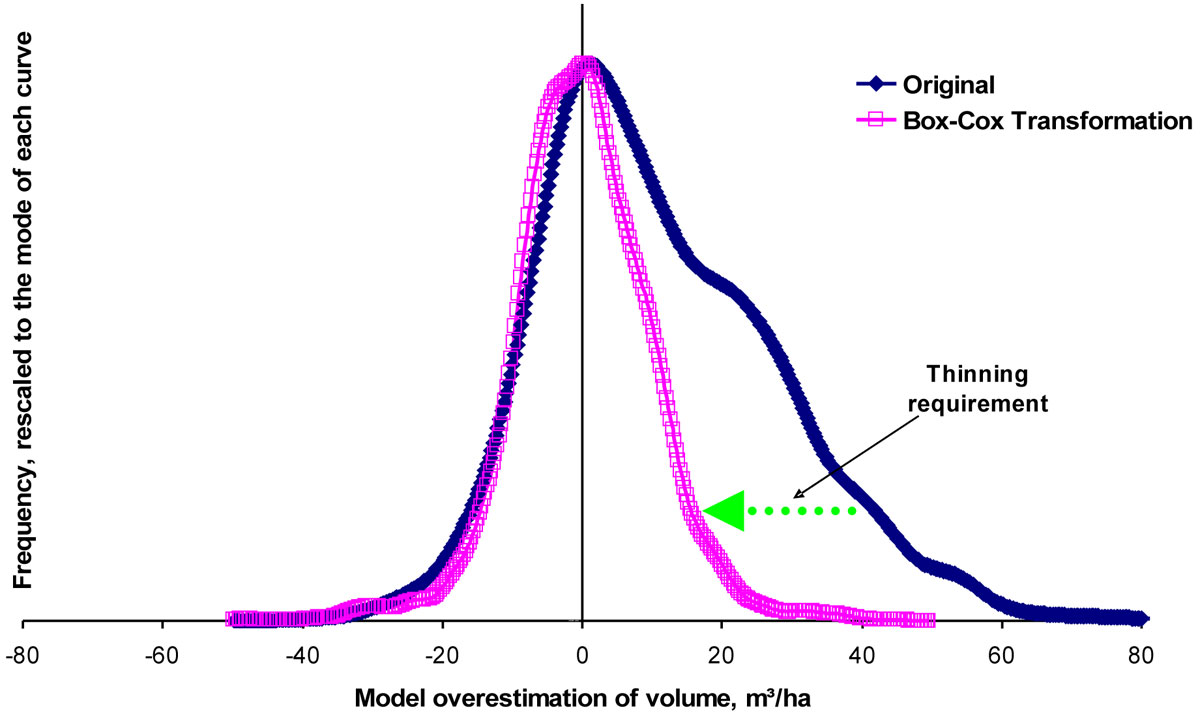
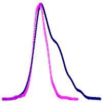
(3) We assume that the mismatch between the NFI biomass estimations and the model outputs should be normally distributed. A Box-Cox power transformation ([2]) was applied to the mismatch data for each species group, and the thinning requirement for each plot calculated as the difference between the mismatch curve and the transformed curve, centred on zero (Fig. 2), less a minor adjustment to compensate for the extra soil nitrogen use in a thinned stand.
Fig. 2 - Relationship of model output to NFI data, by plot. The original “error” curve (closed symbols, dark blue) shows a clear positive skew, reflecting a model overestimation of volume with no assumed thinnings. Applying a Box-Cox power transformation to this curve increases the normalcy of the error distribution (open symbols, pink). The required thinning for any plot (in m³/ha) is the lateral distance between that plot’s corresponding points on the two curves. Note that the transformed curve has been scaled vertically down for this figure, to increase the clarity of the concept.
(4) Removals calculated in step 3 are modelled as thinnings taken place some time prior to Period 1 (although they also may have been partial harvests or significant disturbance events). To avoid these having a biophysical impact on modelling post-Period 1 due to increased nitrogen consumption by soil bacteria, we apply a series of steps to determine reasonable assumptions for the timing of the removals.
- If the stand is over 50 years old, first removal is assumed to be at age 40 ([20]).
- If insufficient biomass can be removed in a single step (required removals are greater than modelled standing biomass), subsequent removals occur at ages 70, 100 and 130 and 5 years prior to the Period 1 inventory date.
- If a subsequent removal is required, the prior removal is limited to 40 percent of biomass.
- A maximum of 95% of biomass may be removed in the final step.
To convert biomass figures to more readily visualised timber volume per hectare values, we compiled a regression of all 33 779 tree measurements in the available dataset, calculating conversion factors between biomass estimates made with allometry and biomass expansion factors developed for Central European species (Lexer, pers. comm. - 10 February 2010) and merchantable timber volume estimates consistent with Pollanschütz ([25]) - Tab. 1. All species are included here, as some of our 1133 plots contained a minor component of other species. It should be noted however that for species other than those in our major groups often few data points were available for the biomass/timber volume regression, and thus the multipliers may be unreliable for those species. The Lexer equations were used for consistency with concurrent studies ([35]), as the only available comprehensive estimates for Austrian conditions.
Tab. 1 - Multipliers for conversion of above-ground woody biomass (kg/m2) to volume (m3/ha) consistent with Pollanschütz ([25]).
| Species | Multiplier | Species | Multiplier |
|---|---|---|---|
| Spruce (Picea abies), low elevation | 18.91 | Chestnut (Castanea sativa) | 12.31 |
| Fir (Abies alba) | 18.28 | Black Locust (Robinia pseudoacacia) | 11.11 |
| Larch (Larix decidua) | 21.46 | Sorbus/Prunus spp. | 9.94 |
| Scots Pine (Pinus sylvestris) | 22.12 | Birch (Betula spp.) | 11.01 |
| Black Pine (Pinus nigra) | 18.29 | Black Alder (Alnus glutinosa) | 16.93 |
| Stone Pine (Pinus cembra) | 7.45 | White Alder (Alnus incana) | 10.66 |
| Douglas Fir (Pseudotsuga menziesii) | 6.25 | Linden (Tilia cordata) | 15.01 |
| Other conifers | 6.81 | Aspen, Poplars (Populus spp.) | 13.74 |
| Beech (Fraxinus excelsior) | 13.17 | Black Poplar (Populus nigra) | 12.58 |
| Oak (Quercus robur/petraea) | 12.53 | Hybrid Poplars (Populus x spp.) | 11.83 |
| Hornbeam (Carpinus betulus) | 11.61 | Willow (Salix spp.) | 8.95 |
| Ash (Fraxinus excelsior) | 13.61 | Other broadleafs | 9.06 |
| Maple (Acer spp.) | 11.41 | Spruce, high elevation | 15.9 |
| Elm (Ulmus spp.) | 11.53 | - | - |
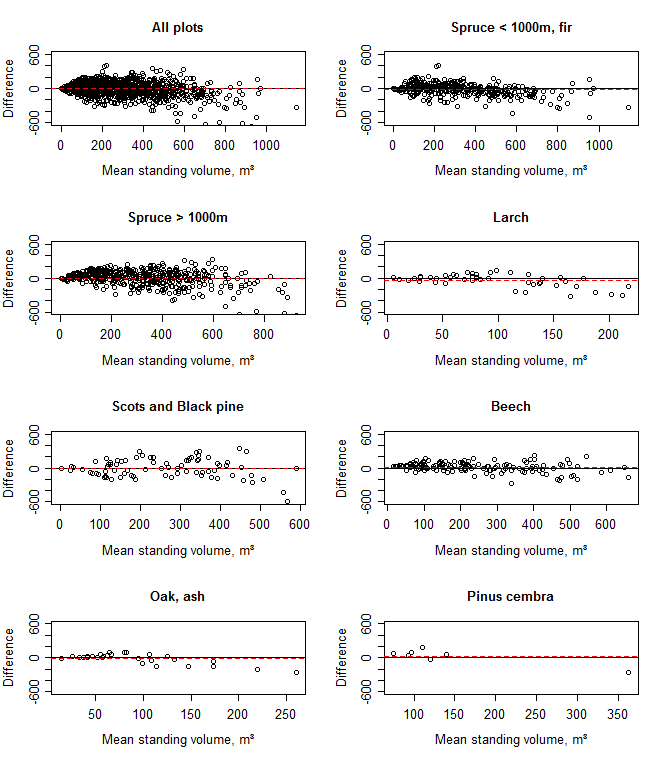
Given the very poor precision of angle-count estimates of volume on single points, a regression of observed versus predicted standing volume is inappropriate. We therefore apply the methods of Bland & Altman ([1]), which for each data point plot the difference between values determined through each method against their mean for each point.
Results and discussion
The initial simulation of forest growth on the NFI plots was performed without any management interventions. A comparison of model outputs with observed data displayed a remarkably even normal curve for those plots where the model appears to underestimate the NFI (the blue line below zero in Fig. 2). This gives some confidence that if management were appropriately considered, the variation between the simulations and the NFI data would also be normally distributed for apparent overestimations.
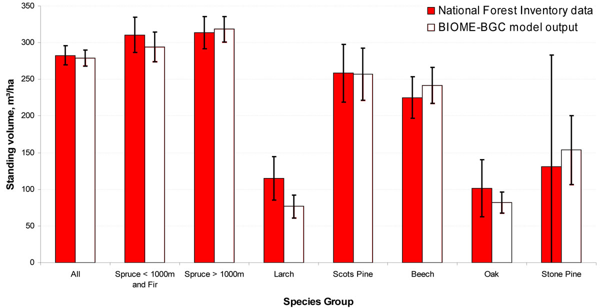
Overall, the procedure enabled a close simulation of standing volume (Fig. 3). Some problems exist with the Larch simulation, probably due to poor species data resulting from the low number of samples used in the initial species parameterisation ([23], Pietsch, pers. comm. - 25 June 2010). Results for the Oak/Ash and Stone Pine groups are rather uncertain due to the low numbers of plots available in this study for those species. The Bland-Altman plots (Fig. 4) show that the errors are consistent over the range of standing volumes, with little evidence of heteroscedasticity.
Fig. 3 - Standing volume in Period 1. Error bars show one standard deviation above and below the mean.
Fig. 4 - Bland-Altman plot of standing volume determined with inventory and with the BIOME-BGC model. In each plot the “x” axis is the mean of the volume assessed with each method, while the “y” axis is the difference between the methods (BGC subtract inventory). Dashed lines indicate the mean difference.
The Lexer biomass equations are based only on dbh. Several authors have presented allometry for major European species in different regions ([13] and [37] for Fagus sylvatica, [36] for Picea abies and [3], [5] for Pinus sylvestris and Quercus spp. respectively). All of these authors concluded that allometric models can be considerably improved by including height and other variables, rather than basing results solely on dbh. The Austrian NFI however contains many records where height is calculated from dbh rather than directly measured, which would appear to negate any possible advantage of using more complicated allometrics.
Besides natural variability, several other factors may account for the differences between model output and NFI records. The version of BIOME-BGC we use in this study is not designed to simulate mixed-species forest, so the up to 20 percent of non-homogenous species on any plot may have some minor effect. Uncertainty in biomass expansion factors ([16]) is also possibly biasing on some plots, where the by-plot ratio of volume to biomass is not the same as the mean by-tree relationship for the dominant species (Tab. 1).
Although it may seem that the results presented here are an artificial “forcing” of model assumptions to match the NFI data, in most cases the simulated thinnings are timed to occur several decades prior to the inventory measurement. The model is thus required to accurately simulate growth over long periods before the results in Fig. 3 are extracted. Alternative approaches such as thinning to precisely match field data ([28]) would not be possible for apparent model underestimations and thus would give an underestimation in the mean. Thinning all plots equally so that the simulation and the field data have equal means would simply shift the blue curve in Fig. 1 to the left, giving a non-normal error distribution. An “expert opinion” approach ([20]) would ignore the standing volume information available in the NFI dataset. Although single plot data in the NFI is extremely imprecise, in the aggregate it can be assumed to provide accurate values.
By thinning to target a normal error curve, apparent model underestimations are little affected. In cases where a plot simulated without thinning greatly overestimates standing volume a heavy or a series of thinnings is indicated. There are any number of possible normal error curves that could have been selected as the “target” error curve, but the procedure using the Box-Cox transformation was chosen to maximise the use of the available data. The timing of the thinning events at 40, 70, 100 and 130 years of age appears to be reasonably consistent with records from the NFI (Fig. 5). A breakdown of thinning volume removals (Tab. 2) suggests that the assumption procedure tends to underestimate the number of thinnings, but overestimate the volume removed in each thinning event. The results shown in Fig. 3 however suggest that this has a minimal effect on the final simulated standing volumes.
Fig. 5 - Frequency of removal events in each age class between the first two periods of the modern Austrian National Forest Inventory. Tick marks on the “x” axis correspond to the assumed timing of thinnings for BIOME-BGC model initialization.
Tab. 2 - Comparison of determined thinning assumptions with NFI records between the first and second modern Austrian National Forest Inventory periods. Inventory values for the number of thinning events and the sum of volume removed are the annual mean of the 5-year inter-period, while the assumptions values are the annual mean of the 20 years from 1961-1980.
| Group | Inventory | Thinning assumptions | ||||
|---|---|---|---|---|---|---|
| n yr-1 | mean (m3 ha-1) |
sum (m3 ha-1yr-1) |
n yr-1 | mean (m3 ha-1) |
sum (m3 ha-1yr-1) |
|
| All | 46.00 | 55.27 | 2542.33 | 22.95 | 69.24 | 1589.10 |
| Spruce < 1000m and fir | 21.20 | 55.22 | 1170.69 | 12.60 | 84.01 | 1058.55 |
| Spruce > 1000m | 15.00 | 64.25 | 963.75 | 6.55 | 53.10 | 347.80 |
| Larch | 0.20 | 15.17 | 3.03 | 0.00 | 0.00 | 0.00 |
| Scots pine | 4.00 | 42.01 | 168.02 | 0.15 | 23.67 | 3.55 |
| Beech | 5.00 | 42.04 | 210.20 | 3.65 | 49.10 | 179.20 |
| Oak/ash | 0.40 | 51.47 | 20.59 | 0.00 | 0.00 | 0.00 |
| Stone pine | 0.20 | 30.24 | 6.05 | 0.00 | 0.00 | 0.00 |
Conclusions
The incorporation of unknown forest management histories into ecosystem modelling is a challenging issue, yet the ability of models to accurately mimic forest volume growth is dependant on management being appropriately considered. As we will rarely know the history of a large number of sites in sufficient detail to use real figures for historic thinnings, supportable procedures must be developed for appropriate assumptions. While National forest inventories provide large datasets of potential calibration data, the statistical nature of inventories means that we cannot assume a single inventory point to be representative of a wider area and directly comparable with model outputs for that point. The statistical estimation of management history in this work does not attempt to describe the real, unknown thinning history of each stand. Rather, it establishes a set of assumptions that can mimic the true management history in such a way that we can produce unbiased estimates of standing volume which, at a sufficiently large scale, are compatible with National Forest Inventories.
The procedure developed here has provided us with model-driven timber volume estimates for 1133 sites across the whole of Austria that are overall a close match to NFI records at the national scale, are of comparable precision, and maximise the use of available data. Future work will examine how well model simulations compare with NFI records for subsequent inventory periods, where statistical indications are available regarding management interventions on each plot.
Acknowledgements
This work was supported by the two projects:Auswirkungen des Klimawandels auf Österreichs Wälder - Entwicklung und vergleichende Evaluierung unterschiedlicher Prognosemodelle (WAMOD) and Comparing satellite versus inventory driven carbon estimates for Austrian Forests (MOTI), both funded by the Energy Fund of the Federal State of Austria and managed by Kommunalkredit Public Consulting GmbH. We thank the two anonymous reviewers and the editor of the journal for helpful suggestions to improve this manuscript.
References
Gscholar
Gscholar
Gscholar
Gscholar
Gscholar
Gscholar
CrossRef | Gscholar
Gscholar
Gscholar
Gscholar
Gscholar
Gscholar
Gscholar
Gscholar
Gscholar
Gscholar
CrossRef | Gscholar
Gscholar
Gscholar
Authors’ Info
Authors’ Affiliation
H Hasenauer
Institute of Silviculture, University of Natural Resources and Life Sciences (BOKU), Vienna (Austria).
Corresponding author
Paper Info
Citation
Eastaugh CS, Hasenauer H (2011). Incorporating management history into forest growth modelling. iForest 4: 212-217. - doi: 10.3832/ifor0597-004
Paper history
Received: Nov 30, 2010
Accepted: Aug 22, 2011
First online: Nov 03, 2011
Publication Date: Nov 03, 2011
Publication Time: 2.43 months
Copyright Information
© SISEF - The Italian Society of Silviculture and Forest Ecology 2011
Open Access
This article is distributed under the terms of the Creative Commons Attribution-Non Commercial 4.0 International (https://creativecommons.org/licenses/by-nc/4.0/), which permits unrestricted use, distribution, and reproduction in any medium, provided you give appropriate credit to the original author(s) and the source, provide a link to the Creative Commons license, and indicate if changes were made.
Web Metrics
Breakdown by View Type
Article Usage
Total Article Views: 58630
(from publication date up to now)
Breakdown by View Type
HTML Page Views: 49417
Abstract Page Views: 3451
PDF Downloads: 4360
Citation/Reference Downloads: 29
XML Downloads: 1373
Web Metrics
Days since publication: 5269
Overall contacts: 58630
Avg. contacts per week: 77.89
Article Citations
Article citations are based on data periodically collected from the Clarivate Web of Science web site
(last update: Mar 2025)
Total number of cites (since 2011): 9
Average cites per year: 0.60
Publication Metrics
by Dimensions ©
Articles citing this article
List of the papers citing this article based on CrossRef Cited-by.
Related Contents
iForest Similar Articles
Research Articles
Modelling the carbon budget of intensive forest monitoring sites in Germany using the simulation model BIOME-BGC
vol. 2, pp. 7-10 (online: 21 January 2009)
Research Articles
Use of BIOME-BGG to simulate Mediterranean forest carbon stocks
vol. 4, pp. 121-127 (online: 01 June 2011)
Commentaries & Perspectives
Reply: “Use of BIOME-BGC to simulate Mediterranean forest carbon stocks”
vol. 4, pp. 249 (online: 03 November 2011)
Research Articles
Deriving tree growth models from stand models based on the self-thinning rule of Chinese fir plantations
vol. 15, pp. 1-7 (online: 13 January 2022)
Commentaries & Perspectives
Comment on Chiesi et al. (2011): “Use of BIOME-BGC to simulate Mediterranean forest carbon stocks”
vol. 4, pp. 248 (online: 03 November 2011)
Research Articles
Modeling of time consumption for selective and situational precommercial thinning in mountain beech forest stands
vol. 14, pp. 137-143 (online: 16 March 2021)
Research Articles
Methods to inventory and strip thin in dense stands of aspen root suckers
vol. 8, pp. 590-595 (online: 22 April 2015)
Research Articles
Use of BIOME-BGC to simulate water and carbon fluxes within Mediterranean macchia
vol. 5, pp. 38-43 (online: 02 April 2012)
Short Communications
Dynamic modelling of target loads of acidifying deposition for forest ecosystems in Flanders (Belgium)
vol. 2, pp. 30-33 (online: 21 January 2009)
Research Articles
Interactions between thinning and bear damage complicate restoration in coast redwood forests
vol. 13, pp. 1-8 (online: 08 January 2020)
iForest Database Search
Search By Author
Search By Keyword
Google Scholar Search
Citing Articles
Search By Author
Search By Keywords
PubMed Search
Search By Author
Search By Keyword

