Deriving tree growth models from stand models based on the self-thinning rule of Chinese fir plantations
iForest - Biogeosciences and Forestry, Volume 15, Issue 1, Pages 1-7 (2022)
doi: https://doi.org/10.3832/ifor3792-014
Published: Jan 13, 2022 - Copyright © 2022 SISEF
Research Articles
Abstract
Self-thinning due to density-dependent mortality usually occurs during the forest development. To improve predictions of such processes during forest successions under climate change, reliable stand-level models are needed. In this study, we developed an integrated system of tree- and stand-level models by deriving tree diameter and survival models from stand growth and survival models based on climate-sensitive self-thinning rule of Chinese fir plantations in subtropical China. The resulting integrated system, having a unified mathematical structure, should provide consistent estimates at both tree and stand levels. Predictions were reasonable at both stand and tree levels. Because stand-level values aggregated from the tree model outputs are different from those predicted directly from the stand models, the disaggregation approach was applied to provide numerical consistency between models of different resolutions. Compared to the unadjusted approach, predictions from the disaggregation approach were slightly worse for tree survival but slightly better for tree diameter. Because the stand models were developed under the climate-sensitive self-thinning trajectory, the integrated system could offer reasonable predictions that could aid in managing Chinese fir plantations under climate change.
Keywords
Chinese Fir, Self-thinning Rule, Disaggregation, Stand Model, Tree Model
Introduction
The self-thinning rule, which describes the relationship between stand density and the average tree size in a situation of density-dependent mortality, continues to attract foresters’ attention ([6]). Variables such as tree biomass ([42]), quadratic mean diameter ([45]), and average height ([7]) have been used to describe tree size in the self-thinning rule. Reineke ([31]) proposed the slope in the self-thinning line (or maximum size-density line) was a constant with value of -1.605. However, the existence of a constant slope has been widely debated ([29], [17]). Several reports argued that the slope may not be universally invariant, changing due to tree species ([12]), initial spacing ([38]), site quality ([5]), and climate conditions ([46]).
Because the self-thinning rule refers to density-dependent mortality, it has been used as the basis for developing stand management diagrams ([38], [35]), constructing density indices ([39]), and especially for predicting forest growth and stand survival ([25]). Note that in this study, stand survival is defined as number of surviving trees per ha.
Forest growth and yield models provide an important basis for managing forest reasonably. These models are categorized into four kinds of models: whole-stand models, size-class models, diameter distribution models, and individual tree-models ([8]). Whole-stand models offer information on the whole stand such as stand basal area ([21]), stand survival ([34]), and stand volume ([20]). Size-class models deal with trees classified into diameter classes. These models include stand-table projection models, which predict the frequency in each diameter class ([26], [1]), and diameter-distribution models, which use a probability density function to model the diameter distributions ([11]). Individual-tree models, on the other hand, provide detailed tree information such as tree diameter growth ([36]), tree survival ([24]), or both ([23]).
In general, for unthinned stands whole-stand models provide more accurate stand-level predictions than individual-tree models, because stand-level predictions aggregated from tree models usually lead to accumulating errors in plantations ([30]). For the same site, a forest manager might prefer stand-level models to predict stand attributes, but might need tree models to aid management decisions that require detailed tree-level information. Because stand-level attributes predicted from tree and stand-level models are numerically inconsistent with each other, disaggregation has been employed as a method for maintaining compatibility between the two types of models ([32]). This method attempts to adjust stand-level variable predictions obtained from individual-tree models such that the aggregated predictions would match the outputs of whole-stand model ([32]).
Chinese fir (Cunninghamia lanceolata (Lamb.) Hook.) is a native coniferous tree species widespread in southern China. It is commonly used for timber production because its straight stem and good resistance to bending and cracking ([47]). The planting area for this species is about 8.95 million hectares, about 30% of all afforestation in China ([22]). Zhang et al. ([45]) used the segmented regression technique to develop the self-thinning model of Chinese fir plantations. The slopes in the self-thinning lines were found to be variable from site to site, and could be predicted by the use of several climate factors ([46]). Based on this work, Zhang et al. ([47]) developed a system of stand basal area, quadratic mean diameter growth, and survival models according to the self-thinning rule. They found that the stand models under the climate-sensitive self-thinning trajectories provided reasonable predictions under climate change.
Daniels & Burkhart ([13]) put forward a concept of the integrated system of forest growth models, all of which having a unified mathematical structure, so as to provide consistent estimates at different level models. This concept has been applied by Cao ([9]) to develop an integrated system to predict stand survival at both tree and stand levels. Cao ([10]) later extended this technique to derive a tree survival model from any existing stand survival models. Thus, it is necessary to derive the tree growth and survival models from the stand models which will improve model predictions and compatibility between stand- and tree-level models.
The objective of this study was to establish an integrated system by deriving individual-tree diameter growth and survival models from stand-level growth and survival models for Chinese fir plantations. The benefits of this integrated system consist of stand-level models that follow the self-thinning rule, and correspond to tree-level models that are flexible for detailed tree growth projection, tree merchandizing, and also for simulation purposes. Because the stand models were climate-sensitive, the integrated system with the above properties should provide reasonable growth and yield predictions that could aid future management of Chinese fir under climate change.
Materials and methods
Study sites and data measurement
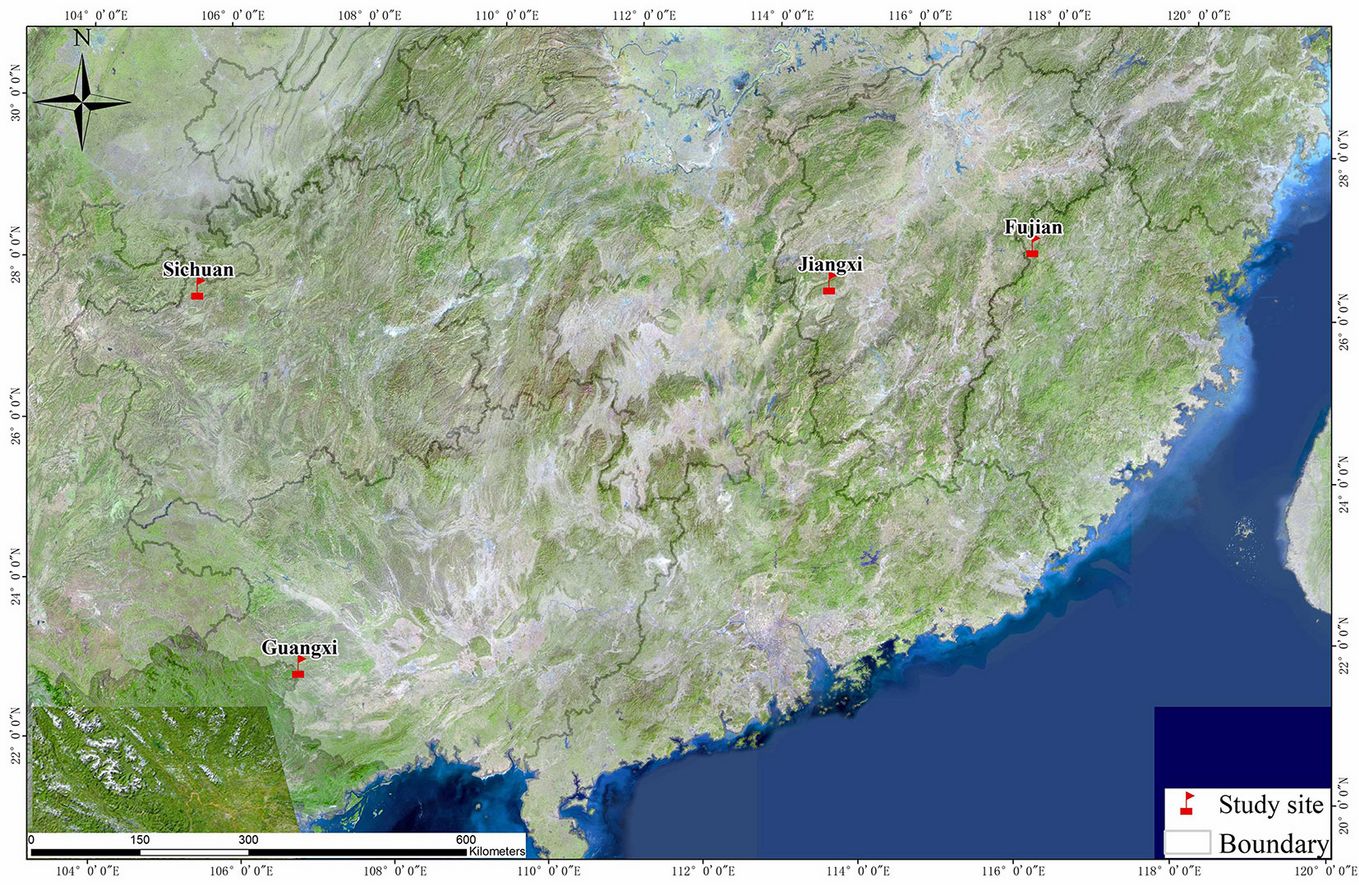
The experimental sites were situated in Fujian, Jiangxi, Guangxi, and Sichuan provinces in southern China. Fujian, Jiangxi, and Sichuan provinces belong to middle-subtropical climate zones, whereas Guangxi has southern-subtropical climate (Tab. 1, Fig. 1). The landforms at the four sites are low mountains and high hills, with elevation ranging from 300 to 500 m a.s.l. Parent rocks in Fujian and Guangxi are Granite. In Jiangxi and Sichuan, parent rocks are sandy shale and shale, respectively. The soil type is mainly Laterite for Fujian, Guangxi, and Sichuan, and is mainly yellow-brown for Jiangxi.
Tab. 1 - Mean annual temperature (MAT), annual precipitation (AP), degree-days below 0° C (DD0), summer mean maximum temperature (SMMT), and winter mean minimum temperature (WMMT) of study period, by site.
| Site | MAT (°C) |
AP (mm) |
DD0 | SMMT (°C) |
WMMT (°C) |
|---|---|---|---|---|---|
| Fujian | 18.90 | 1768 | 1 | 32.18 | 4.75 |
| Jiangxi | 18.04 | 1572 | 2 | 32.01 | 4.23 |
| Guangxi | 22.27 | 1494 | 0 | 31.79 | 12.24 |
| Sichuan | 18.31 | 1179 | 1 | 30.69 | 7.09 |
Fig. 1 - Study sites located in subtropical climate zones in this study.
The plots were planted in 1982 in Fujian, Guangxi and Sichuan, and in the spring of 1981 in Jiangxi. Each site was established with four planting densities: 2 × 1.5 m (3333 trees ha-1), 2 × 1 m (5000 trees ha-1), 1 × 1.5 m (6667 trees ha-1), and 1 × 1 m (10,000 trees ha-1). The experiments were installed in a random block arrangement with three replications for each level. Four plots were distributed in each block (one plot for each spacing trial). In each site, twelve plots (20 × 30 m each) were established. Surrounding each plot there were two rows of trees with the same spacing, which formed a buffer zone.
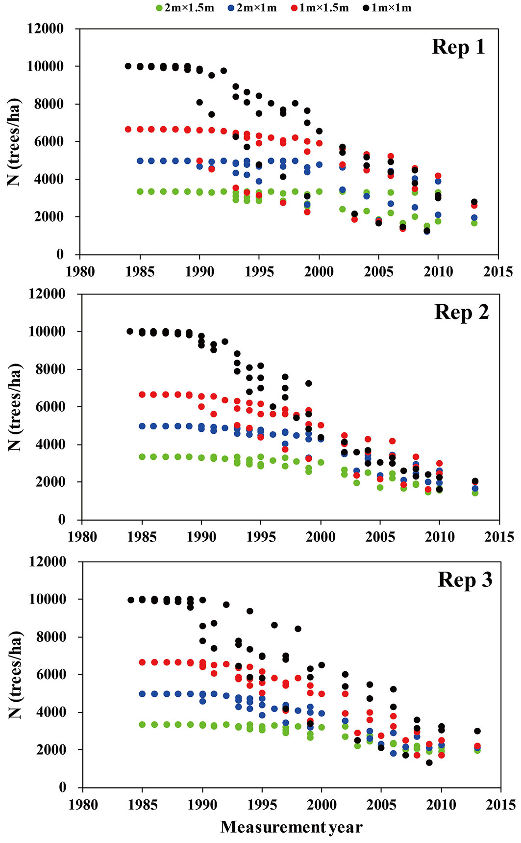
In each plot, diameters at a height of 1.3 m (dbh) of all trees were measured, and over 50 trees were randomly chosen for measuring height. Dominant height was computed as the average height of the six tallest trees in the sample. In 1998, a snowstorm in Jiangxi killed some trees, and therefore the data after 1999 for this site were dropped from this study. The study period ranged from 1985 to 2010 in Fujian, 1985 to 1999 in Jiangxi, 1990 to 2009 in Guangxi, and 1985 to 2013 in Sichuan. Field measurement was done in the winter every 1 to 3 years. Tab. 2 showed the summary statistics of stand and tree factors by replication. Fig. 2 showed the number of trees per ha over time.
Tab. 2 - Summary statistics (mean ± standard deviation) of stand- and tree-level variables of Chinese fir plantations from 1985 to 2013, by replication.
| Variable | Replication 1 | Replication 2 | Replication 3 |
|---|---|---|---|
| A: stand age (years) | 13 ± 6.2 | 12 ± 6.0 | 12 ± 6.0 |
| N: number of trees ha-1 | 6159 ± 2473 | 6120 ± 2495 | 6080 ± 2452 |
| B: stand basal area (m2 ha-1) | 36.12 ± 16.32 | 33.89 ± 16.81 | 36.94 ± 15.34 |
| Q: quadratic mean diameter (cm) | 9.0 ± 3.0 | 8.7 ± 3.2 | 9.2 ± 3.2 |
| H: stand dominant height (m) | 11.1 ± 3.9 | 11.2 ± 4.5 | 11.4 ± 4.1 |
| d: tree diameter at breast height (cm) | 8.7 ± 3.8 | 8.4 ± 3.9 | 8.9 ± 4.0 |
Fig. 2 - Number of trees per ha (N) over time by replication. Fujian: every year from 1985 to 1990; every two years from 1990 to 2010; Jiangxi: every year from 1985 to 1989; every two years from 1989 to 1999; Guangxi: every year from 1990 to 1995; every two years from age 1995 to 2009; Sichuan: every year from 1985 to 1995; every two years from 1995 to 1999 and from 2002 to 2010; every three years from 1999 to 2002 and 2010 to 2013.
Height-age model
The stand-level models (described further below) require projection of dominant height over time. The height-age model developed by Bailey & Clutter ([2]) has been found to perform well in modeling the dominant height growth of Chinese fir (eqn. 1):
where Hit is the dominant height (m) of plot i at year t, Ait is the stand age (years) of plot i at year t, p is the growth period in years, the ^ denotes predicted values, and β1-β2 are parameters to be estimated, with values listed in Zhang et al. ([47]).
Stand-level growth and survival models
Zhang et al. ([47]) developed a system to predict stand quadratic mean diameter growth and survival. The quadratic mean diameter was predicted as follows (eqn. 2):
where Qit is the stand quadratic mean diameter (cm) of plot i at year t, Nit is the number of trees per ha of plot i at year t, and χ0-χ4 are parameters to be estimated.
Prediction of stand survival was based on the climate-sensitive self-thinning model ([46] - eqn. 3 to eqn. 5):
where yit = ln(Nit), xit = ln(Qit), yi0 = ln(Ni0), Ni0 = planting density (number of trees ha-1) for plot i, and (eqn. 6, eqn. 7):
with ci being the self-thinning slope for plot i, given by (eqn. 8):
where c0-c5 are regression parameters, with values listed in Zhang et al. ([46]), MAT is the mean annual temperature, AP is the annual precipitation, DD0 are the degree-days below 0 °C, SMMT is the mean maximum temperature of months in summer, WMMT is the mean minimum temperature of winter months, and α1-α3 are the parameters to be estimated.
Stand basal area is computed using stand quadratic mean diameter and survival (eqn. 9):
where {hat}Bi,t+1 is the stand basal area prediction (m2 ha-1) of plot i at year t+1, and K=π/40000.
Tree-level growth and survival models
Given the above stand-level models, individual tree models can be derived from their outputs. Tree diameter was obtained from the predicted quadratic mean diameter as follows (eqn. 10):
where dij,t is the tree diameter (cm) at 1.3 m height of tree j in plot i at year t, and χ5 is a tree-level parameter to be estimated (see further below).
Cao ([10]) derived a tree survival model based on stand survival prediction. The tree survival probability, expressed as a function of current quadratic mean diameter and current and future number of trees per ha, is listed below in annual form (eqn. 11):
where Pij,t+1 is the tree survival probability prediction of tree j nested in plot i at year t+1, and δ1-δ3 are parameters to be estimated. Eqn. 7 and eqn. 8 form the tree-level models, with parameters χ5, δ1, δ2, and δ3 to be estimated from the tree data.
Because of different growth intervals, the annual growth projection method was used to model the survival and growth models to ensure the step-invariance property of the predictions. Stand-level models were predicted annually in a recursive way: quadratic mean diameter and stand survival were projected repeatedly from equations for Q and y from age t1 to t2, from t2 to t3, and so on until the end of the growing period. The tree-level models can be derived either at each intermediate age or at the end of the growth period.
Parameter estimation
The Sequential Estimation approach ([9]) was employed in this study. This approach involves estimating parameters sequentially, with some parameters estimated at the stand level and the remaining parameters at the tree level. At the stand-level phase, parameters in equations for Q, y, and B were estimated via the Seemingly Unrelated Regression (SUR) method using the procedure MODEL in SAS ([33]). At the tree-level phase, parameters in equations for p and d were estimated using the maximum likelihood approach.
Disaggregation
Outputs from the stand-level models were often different in values from stand outputs aggregated from tree-level models. The following disaggregation method ([9]) was used for adjusting tree survival and diameter predictions. The advantage of disaggregation is that the aggregated values from the tree models after adjustment matched the stand basal area and survival predictions from the stand-level models, resulting in a numerically consistent system.
Tree survival probability was adjusted as follows (eqn. 12):
where {tilde} Pij,t+p and Pij,t+p are, respectively, adjusted and predicted tree survival probability of tree j nested in plot i at the end of the growth interval t+p, λ is the adjusting parameter, which is iteratively solved through (eqn. 13):
with Nij,t+p being the stand survival predicted from the stand survival model, and s is the plot size in hectares. Adjustments for future tree diameters were done as follows (eqn. 14):
where {tilde}dij,t+p and {tilde}dij,t+p are, respectively, adjusted and predicted diameter of tree j in plot i at year t+p, dij,t is the observed diameter of jth tree nested in plot i at year t, and (eqn. 15):
and {tilde}Bi,t+p is the stand basal area obtained from eqn. 6.
Model evaluation
Here, a three-fold cross-validation approach was applied for validating the growth and survival models at both stand and tree levels. Parameter estimates from two replications (fit data) were used to predict the growth and survival of the remaining replication (validation data). Then the procedure was repeated for all the subsets and the final validation data consisted of all replications. Three evaluation statistics, namely mean error (ME), mean absolute error (MAE) and fit index (R2) were calculated for stand basal area and survival prediction as well as tree diameter prediction (eqn. 16 to eqn. 18):
where yi indicates the observed N, B, Q, or d of the observation i, n indicates the number of observations, and {bar}y and {hat}y are average and predicted values of N, B, Q, and d, respectively.
For tree survival prediction, three evaluation statistics were used, namely ME (mean error), MAE (mean absolute error) and AUC (eqn. 19 to eqn. 20):
where yij = 1 if the j-th tree nested in i-th plot survived at the end of the growth interval, and yij = 0 otherwise; Pij is the predicted tree survival probability; n1i is number of trees ha-1 in ith plot at the start of the growth interval. AUC is the area under the receiver operating characteristic curve (AUC) commonly applied for evaluating tree mortality model ([14]). It ranged from 0.5 to 1. The model with larger AUC indicates the tree mortality model performed better.
Results and discussions
Integrated system of tree- and stand-level models
Tab. 3showed the parameter estimates of the growth and survival models in both stand and tree levels, which showed that all parameters of these models were significant at α = 0.05. Outputs from the stand-level models yielded consistently higher values of R2 and smaller values of MAE as compared to aggregated outputs from the unadjusted tree-level models (Tab. 4). Direct prediction of stand variables apparently was preferable to aggregating tree-level outputs. This result is consistent with the findings by Qin & Cao ([30]) who predicted stand basal area, survival, and volume of loblolly pine (Pinus taeda Linn.), Zhang et al. ([43]) who predicted stand basal area and survival of Chinese pine (Pinus tabuliformis Carr.) in China, and Hevia et al. ([19]) who predicted stand survival and basal area of birch-dominated stands in Spain. García ([16]) reported that problems of accumulation of errors tend to be more serious when aggregating tree-level outputs.
Tab. 3 - Parameter estimates (± standard errors) of the stand- and tree-level growth and survival models by group. All parameters were significant at the 0.05 level. (Group 1): not containing replication 1; (Group 2): not containing replication 2; (Group 3): not containing replication 3.
| Models | Parameter | Group 1 | Group 2 | Group 3 |
|---|---|---|---|---|
| Stand-level models | α1 | 5.8134 ± 0.6049 | 5.5446 ± 0.5935 | 5.5420 ± 0.5735 |
| α2 | -0.4423 ± 0.0686 | -0.4052 ± 0.0672 | -0.4158 ± 0.0653 | |
| α3 | -1.9376 ± 0.2896 | -2.7626 ± 0.4705 | -1.8974 ± 0.2831 | |
| χ0 | 5.1654 ± 0.9406 | 5.1133 ± 0.8885 | 6.8275 ± 0.8285 | |
| χ 1 | 0.0654 ± 0.0102 | 0.0539 ± 0.0096 | 0.0618 ± 0.0091 | |
| χ 2 | 0.0469 ± 0.014 | 0.0664 ± 0.0156 | 0.0843 ± 0.0153 | |
| χ 3 | -0.0809 ± 0.0303 | -0.0939 ± 0.0311 | -0.1506 ± 0.0315 | |
| χ 4 | -0.3693 ± 0.0929 | -0.3701 ± 0.0855 | -0.5384 ± 0.0816 | |
| Tree-level models | δ1 | -0.5005 ± 0.0068 | -0.5028 ± 0.0071 | -0.4742 ± 0.0068 |
| δ2 | 0.9963 ± 0.0309 | 1.2017 ± 0.0434 | 0.9410 ± 0.0337 | |
| δ3 | 0.9138 ± 0.0123 | 0.8329 ± 0.0145 | 0.9341 ± 0.0144 | |
| χ 5 | 0.9989 ± 0.0008 | 1.0099 ± 0.0008 | 1.0011 ± 0.0008 |
Tab. 4 - Evaluation statistics for prediction of stand variables from stand-level models and tree-level models (before adjustment). Numbers in italic denote the best statistics for that variable.
| Variable | Type of model |
Mean error (ME) |
Mean absolute error (MAE) |
Fit index (R2) |
|---|---|---|---|---|
| N: Number of trees ha-1 | Stand-level | 3.5358 | 181.646 | 0.9836 |
| Tree-level | -56.1225 | 206.089 | 0.9762 | |
| B: Stand basal area (m2 ha-1) | Stand-level | 1.7019 | 3.7775 | 0.8915 |
| Tree-level | 0.5531 | 4.3241 | 0.8171 | |
| Q: Quadratic mean diameter (cm) | Stand-level | 0.2503 | 0.4835 | 0.9633 |
| Tree-level | 0.2437 | 0.4854 | 0.9632 |
A logical step would be to adjust the tree-level outputs to match the aggregated values with outputs from stand-level models. For many years, the disaggregation method has been used to link tree- and stand-level models. It not only ensured compatibility regarding stand-level outputs, but also yielded better tree-level predictions than the unadjusted approach in former studies ([19]). Qin & Cao ([30]) found that the success of the disaggregated tree-level predictions depends largely on the precision of the stand-level model.
Tab. 5shows that the tree-level diameter and survival models derived from the stand growth and survival models performed well. The disaggregated method for tree diameter produced a larger value of R2 (0.9468 vs. 0.9434) and a lower value of MAE (0.5528 vs. 0.6017) than did the unadjusted method. This result was supported by Qin & Cao ([30]) for tree diameter prediction and Hevia et al. ([19]) for tree basal area prediction. Conversely, the disaggregation method for tree survival yielded lower AUC value (0.8736 vs. 0.8907) and larger MAE value (0.0791 vs. 0.0745) as compared to the unadjusted method (Tab. 5). The result of tree survival prediction was contrary to findings from previous studies, which reported superior performance of the disaggregation method ([44]). The different findings may be due to the ecological differences among the studied species. However, the above results show similar overall performances between the adjusted and unadjusted tree models in terms of predicting tree attributes. The advantage of disaggregation in this study lies in achieving numerical consistency between tree- and stand-level models in predicting stand attributes.
Tab. 5 - Model evaluation statistics of tree diameter growth and survival probabilities models using the three-fold cross-validation by method.
| Method | Tree diameter | Tree survival probability | ||||
|---|---|---|---|---|---|---|
| ME | MAE | R2 | ME | MAE | AUC | |
| Unadjusted | 0.1521 | 0.6017 | 0.9434 | -0.0011 | 0.0745 | 0.8907 |
| Disaggregated | 0.3097 | 0.5528 | 0.9468 | 0.0068 | 0.0791 | 0.8736 |
Daniels & Burkhart ([13]) put forward the concept of an integrated system of unified mathematical structure, which can predict forest growth at any level of resolution. The system developed in this study can consistently predict growth and survival at both tree and stand levels. In addition, because the stand models were based on the climate-sensitive self-thinning rule, the tree-level diameter and survival models derived from these stand models should provide reasonable predictions under climate change.
Model predictions under the self-thinning rule
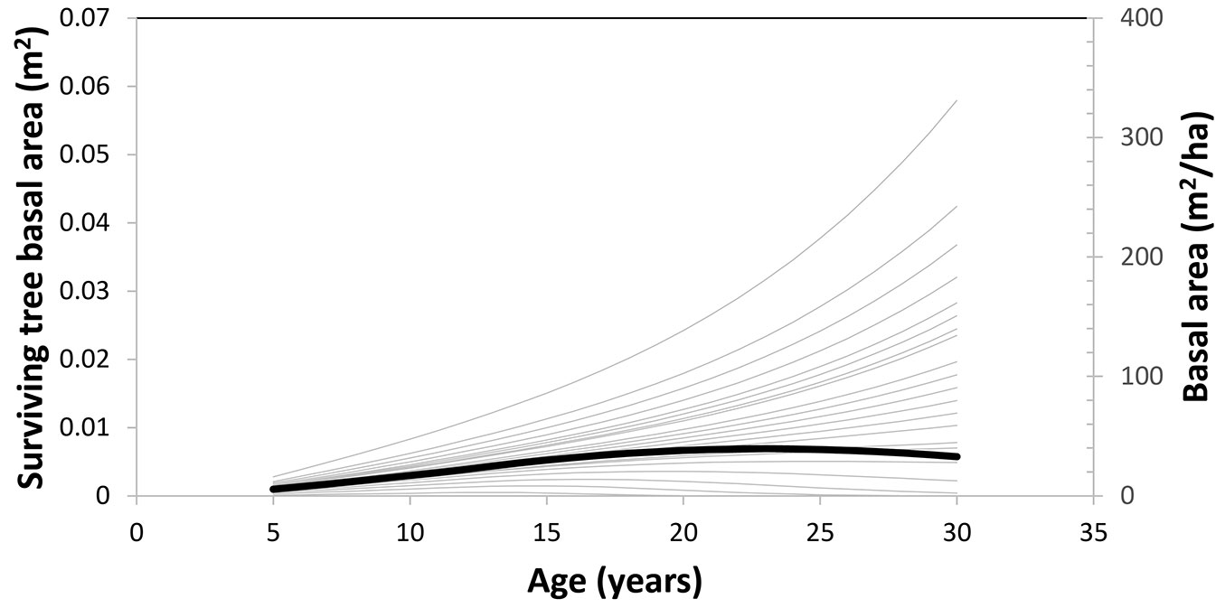
Fig. 3displays the change of tree survival probability over time for various diameter percentiles. This figure is based on the plot located in the Fujian province. In this plot, a tree at each 5% diameter percentile at age 5 was grown to age 30. The graph shows that stand survival rate is equal to tree survival probability at approximately the 20% diameter percentile. A similar graph was drawn for tree survival basal area in Fig. 4. Change in stand basal area over time is therefore a result of two opposing trends: quadratic mean diameter always increases with time, whereas number of trees is unchanged at first, then begins to decrease with time, and finally follows the self-thinning line. Stand basal area, which is a function of the product of N and Q2, increases with time, then stabilizes, and finally decreases (Fig. 4). Surviving tree basal area (computed as survival probability × tree basal area) behaves differently for different diameter sizes; it increases with time for large diameters, or increases, stabilizes, then decreases with time for small diameters.
Fig. 3 - Change of tree survival probability over time (thin curve) for various diameter percentiles, from 0% to 100%, by 5% intervals for a plot in the Fujian province. The lowest thin curve corresponds to the 0% diameter percentile, and the top curve corresponds to the 100% diameter percentile. The dark curve denotes stand survival rate.
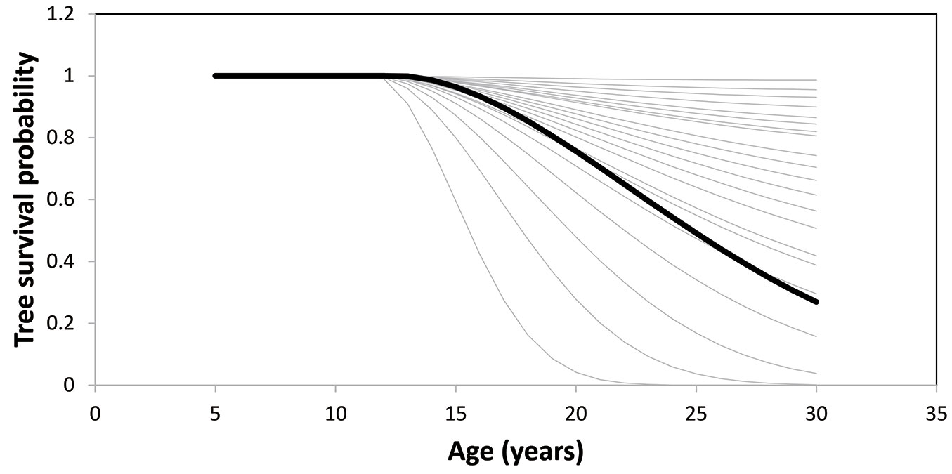
Fig. 4 - Change of tree survival basal area over time (thin curve) for various diameter percentiles, from 0% to 100%, by 5% intervals for a plot. The lowest curve corresponds to the 0% diameter percentile. Tree survival basal area is the product of survival probability and basal area of that tree. The dark curve shows change of stand basal area over time.
Self-thinning usually occurs when the competition for resources (light, nutrient, water, etc.) leads to tree death. Many researchers have used the logistic equation to model tree mortality ([15], [41]). However, if the data sets used to develop mortality equations are from short-term remeasurement data, mortality probabilities predicted without considering the self-thinning rule might be compromised by other factors such as drought, frost, snow, etc., which can lead to an increase in prediction errors. Small changes of tree mortality can profoundly influence forest structure ([40]). Therefore, underestimation of mortality probabilities would cause unreasonably high estimates of forest growth and yield and vice versa. Hann & Wang ([18]) combined the tree mortality equation with the maximum density function of Douglas-fir (Pseudotsuga menziesii (Mirb.) Franco) stands with the objective to produce reasonable tree mortality predictions. Berger et al. ([3]) developed the “Kiwi” model that incorporated the self-thinning rule in studying mangrove forest dynamics, and argued that different self-thinning trajectories must be expected because of competition strength of different tree species. In simulating tree-specific mortality, Monserud et al. ([25]) found that self-thinning controlled mortality and provided feasible model predictions. Tang et al. ([37]) combined the self-thinning and basal area increment models to predict stand density and average diameter, and concluded that the models can be applied to predict stand growth outside the range of the data. Good results were obtained by Ogawa et al. ([28]) and Ogawa ([27]) for leaf biomass models of hinoki cypress (Chamaecyparis obtusa [Sieb. et Zucc.] Endl.), and Zhang et al. ([47]) for stand basal area, quadratic mean diameter, and survival of Chinese fir. In the study by Zhang et al. ([47]), stand basal area increased with time, then stabilized, and finally decreased. This confirmed that productivity loss is balanced by gross productivity during the self-thinning process ([4]). The above literature confirms the benefit of incorporating underlying biological principles such as self-thinning into the development of growth and yield models. Because the system of stand models and their derived tree models in this study was based on the self-thinning rule, it is expected to provide reasonable projections outside the range of the data.
Conclusions
In this study, we developed an integrated system of tree- and stand-level models by deriving tree diameter and survival models from stand growth and survival models. Predictions were reasonable at both stand and tree levels. In addition, the disaggregation approach was applied to provide numerical consistency between models of different resolutions. Compared to the unadjusted approach, predictions from the disaggregation approach were slightly worse for tree survival but slightly better for tree diameter. The advantage of disaggregation in this study lies in achieving numerical consistency between tree- and stand-level models in predicting stand attributes. The stand-level models, based on the self-thinning rule, were compatible with the underlying biological principles. Because they also included climate variables, these stand models and their derived tree-level models formed an integrated system that could offer reasonable predictions for scenarios beyond the data range. Future applications, including those which simulate various climate scenarios, that take advantage of this integrated system could play an important role in managing Chinese fir plantations under climate change.
Acknowledgements
XQ analyzed, conceived, and wrote the draft; QV analyzed, reviewed, and improved the draft; YC analyzed the data; JG conceived the study.
Funding
The study was supported by the National Key Research and Development Program of China (2021YFD2201304) and the National Natural Science Foundation of China (no. 31971645). Partial support for data analysis was received from the National Institute of Food and Agriculture, U.S. Department of Agriculture, Mclntire-Stennis project LAB94379. The authors thank Dr. Aiguo Duan for the field work.
References
Gscholar
Gscholar
Gscholar
Gscholar
Gscholar
Authors’ Info
Authors’ Affiliation
Yancheng Qu
Jianguo Zhang
Key Laboratory of Tree Breeding and Cultivation of the National Forestry and Grassland Administration, Research Institute of Forestry, Chinese Academy of Forestry, Beijing 100091 (P. R. China)
Collaborative Innovation Center of Sustainable Forestry in Southern China, Nanjing Forestry University, Nanjing, 210037 (P. R. China)
School of Renewable Natural Resources, Louisiana State University (USA)
Corresponding author
Paper Info
Citation
Zhang X, Cao QV, Qu Y, Zhang J (2022). Deriving tree growth models from stand models based on the self-thinning rule of Chinese fir plantations. iForest 15: 1-7. - doi: 10.3832/ifor3792-014
Academic Editor
Alessio Collalti
Paper history
Received: Feb 24, 2021
Accepted: Nov 17, 2021
First online: Jan 13, 2022
Publication Date: Feb 28, 2022
Publication Time: 1.90 months
Copyright Information
© SISEF - The Italian Society of Silviculture and Forest Ecology 2022
Open Access
This article is distributed under the terms of the Creative Commons Attribution-Non Commercial 4.0 International (https://creativecommons.org/licenses/by-nc/4.0/), which permits unrestricted use, distribution, and reproduction in any medium, provided you give appropriate credit to the original author(s) and the source, provide a link to the Creative Commons license, and indicate if changes were made.

Web Metrics
Breakdown by View Type
Article Usage
Total Article Views: 12735
(from publication date up to now)
Breakdown by View Type
HTML Page Views: 5961
Abstract Page Views: 3831
PDF Downloads: 2341
Citation/Reference Downloads: 3
XML Downloads: 599
Web Metrics
Days since publication: 1630
Overall contacts: 12735
Avg. contacts per week: 54.69
Article Citations
Article citations are based on data periodically collected from the Clarivate Web of Science web site
(last update: Mar 2025)
Total number of cites (since 2022): 7
Average cites per year: 1.75
Publication Metrics
by Dimensions ©
Articles citing this article
List of the papers citing this article based on CrossRef Cited-by.
Related Contents
iForest Similar Articles
Research Articles
Developing a stand-based growth and yield model for Thuya (Tetraclinis articulata (Vahl) Mast) in Tunisia
vol. 9, pp. 79-88 (online: 23 June 2015)
Research Articles
Long-term effects of thinning and mixing on stand spatial structure: a case study of Chinese fir plantations
vol. 14, pp. 113-121 (online: 08 March 2021)
Research Articles
Modeling stand mortality using Poisson mixture models with mixed-effects
vol. 8, pp. 333-338 (online: 05 September 2014)
Research Articles
Developing stand transpiration model relating canopy conductance to stand sapwood area in a Korean pine plantation
vol. 14, pp. 186-194 (online: 14 April 2021)
Research Articles
Incorporating management history into forest growth modelling
vol. 4, pp. 212-217 (online: 03 November 2011)
Research Articles
Estimation of stand crown cover using a generalized crown diameter model: application for the analysis of Portuguese cork oak stands stocking evolution
vol. 9, pp. 437-444 (online: 02 December 2015)
Research Articles
Spatio-temporal modelling of forest monitoring data: modelling German tree defoliation data collected between 1989 and 2015 for trend estimation and survey grid examination using GAMMs
vol. 12, pp. 338-348 (online: 05 July 2019)
Research Articles
Predicting total and component biomass of Chinese fir using a forecast combination method
vol. 10, pp. 687-691 (online: 17 July 2017)
Research Articles
Modeling of time consumption for selective and situational precommercial thinning in mountain beech forest stands
vol. 14, pp. 137-143 (online: 16 March 2021)
Research Articles
Modelling the carbon budget of intensive forest monitoring sites in Germany using the simulation model BIOME-BGC
vol. 2, pp. 7-10 (online: 21 January 2009)
iForest Database Search
Search By Author
Search By Keyword
Google Scholar Search
Citing Articles
Search By Author
Search By Keywords
PubMed Search
Search By Author
Search By Keyword


