Use of BIOME-BGG to simulate Mediterranean forest carbon stocks
iForest - Biogeosciences and Forestry, Volume 4, Issue 3, Pages 121-127 (2011)
doi: https://doi.org/10.3832/ifor0561-004
Published: Jun 01, 2011 - Copyright © 2011 SISEF
Research Articles
Abstract
BIOME-BGC is a bio-geochemical model capable of estimating the water, carbon and nitrogen fluxes and storages of terrestrial ecosystems. Previous research demonstrated that, after proper calibration of its ecophysiological parameters, the model can reproduce the main processes of Mediterranean forest types. The same investigations, however, indicated a model tendency to overestimate woody biomass accumulation. The current paper aims at modifying BIOME-BGC ecophysiological settings to improve the simulation of the woody compartment in Mediterranean forests. The modified ecophysiological parameter is the whole-plant mortality fraction (WPMF), which directly affects the amount of woody biomass stored. The optimal WPMFs of six main forest types in Tuscany are identified by forcing the model to reproduce the maximum standing volumes found in regional and local forest inventories. The effects of this operation are evaluated by comparing the model outputs produced using the original and modified settings to independent measurements from national forest inventories. The results obtained demonstrate the effectiveness of the modifications introduced and consolidate the methodological basis for extending the use of the modeling strategy to other Mediterranean areas.
Keywords
Mediterranean forest, BIOME-BGC, Stem volume, Current annual increment
Introduction
In the last decades, bio-geochemical models have been used to quantify forest carbon dynamics and monitor the main fluxes and stocks within terrestrial ecosystems ([28]). These models are based on the current knowledge of major ecological/biophysical processes, but generally suffer from high complexity, difficult calibration and great computational intensity ([3], [15]).
These problems are partly overcome by the BIOME-BGC model ([22]) which has been widely applied to quantify water, carbon and nitrogen cycles in different forest ecosystems (e.g., [29], [25]). This model relies on a spin-up phase which defines the local equilibrium conditions for some main biome types (e.g., evergreen needle leaf, deciduous broadleaf, etc.). In general, however, the application of BIOME-BGC to specific ecosystems requires a calibration aimed at properly setting its main ecophysiological parameters ([14]). This is particularly the case for Mediterranean environments, which are characterized by a high spatial heterogeneity of their main properties and by a marked dryness during part of the growing season ([2]).
Recent investigations of our research group showed that BIOME-BGC can be efficiently integrated within a more general modeling strategy for the effective simulation of both water and carbon fluxes and storages in Tuscany forests ([17], [18]). The same studies, however, indicated a model tendency to overestimate woody biomass stocks, which had already been noted by other authors for different European areas (e.g., [20]). This tendency is evidently due to a model deficiency in simulating long-term carbon storages in the woody ecosystem compartment (mostly stems and coarse roots).
The current paper presents an approach to overcome this limitation based on the modification of the model parameter settings which regulate these processes. Specifically, a model parameter which controls biomass storage in woody tissues is adjusted to reproduce the maximum standing volumes measured by regional and local forest inventories. The results of this modification are evaluated by comparison with measurements of forest cover (FC) and current annual increments (CAI) derived from independent inventory sources.
The paper first provides a description of the study region (Tuscany, Central Italy) and of the input data-layers. The methodology section then introduces the modeling strategy based on BIOME-BGC and the procedure applied to improve the model parameter settings. The paper is concluded by the presentation of the results achieved and by a discussion section.
Study area
Tuscany extends over about 9°-12° E long., 42°-44° N lat. The topography of the region ranges from flat areas near the coast-line and along the principal river valleys, to hilly and mountainous zones towards the Apennines chain. Approximately 2/3 of the region is covered by hilly areas, 1/5 by mountains and only 1/10 by plains and valleys. From a climatic viewpoint, the climate ranges from typically Mediterranean to temperate warm or cool according to the altitudinal and latitudinal gradients and the distance from the sea ([21]).
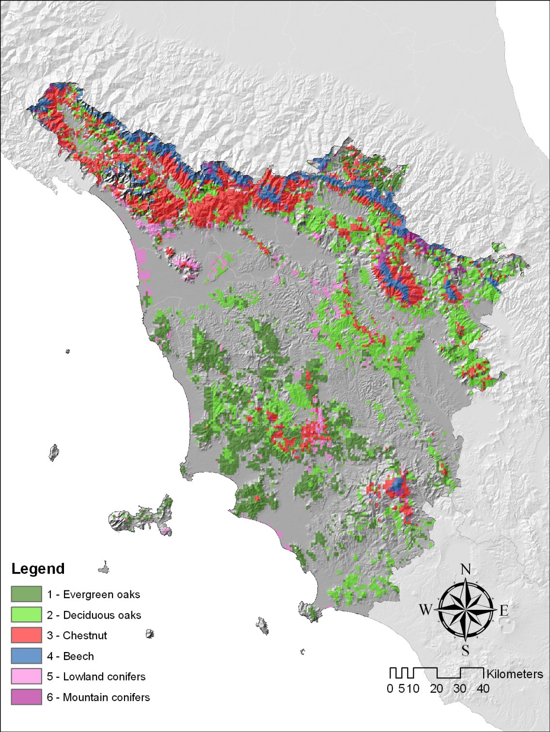
Forests cover approximately half of the regional surface and are mainly located over hilly and mountain areas (Fig. 1). The main forest formations are dominated by various oak forest types (Q. ilex L., Q. pubescens Willd., Q. cerris L.), Mediterranean pines (Pinus pinea L., P. pinaster Ait.), chestnut (Castanea sativa Mill.), beech (Fagus sylvatica L.), silver fir (Abies alba Mill.) and other minor coniferous and deciduous species (Pinus nigra Arnold, Ostrya carpinifolia Scop., Robinia pseudoacacia L., Pseudotsuga menziesii Franco and Cupressus sempervirens L.).
Fig. 1 - Map of Tuscany forests grouped into 6 main forest types (FTs - FT 1: evergreen oaks; FT 2: deciduous oaks; FT 3: chestnut; FT 4: beech; FT 5: lowland conifers; FT 6: mountain conifers), superimposed on a digital illumination model.
Data sources
Forest inventory data
A regional forest inventory (IFT) was carried out in Tuscany during the years 1990-1998 ([1]). This inventory provided point measurements of all main forest attributes collected over a regular 400 m spaced grid. Data from other two local inventories are available for the forests of San Rossore ([8]) and Vallombrosa ([5]).
A more recent national forest inventory (INFC), carried out during the years 2000-2008, provided similar data aggregated on a regional basis for all main forest types in Italy ([12], [13]).
Additional information was derived from CONECOFOR, a project carried out all over Italy aiming at monitoring the status of forests ([11]). In particular, this project reported mean estimates of crown transparency for the main Italian forest classes.
Ancillary data layers
Daily meteorological data were derived from the Tuscany weather network for the years 1996-2008. Distinctively, daily maximum and minimum temperatures and daily total precipitation were collected from 139 and 179 stations spread all over the regional territory, respectively.
A Digital Terrain Model (DTM) of the study region with 1-km spatial resolution was derived from the Regional Cartographic Service of Tuscany. The same Service provided the digital forest map produced by Arrigoni et al. ([1]). This map describes the distribution of 18 different forest classes at 1:250.000 spatial resolution. These classes were regrouped into 6 main forest types (FT) following auto-ecological criteria: evergreen oaks, deciduous oaks, chestnut, beech, lowland conifers and mountain conifers. The main characteristics of the six FTs are shown in Tab. 1.
Tab. 1 - List of the six forest types (FTs) considered with indication of the biome types and of the relevant GPP averages simulated by BIOME-BGC in Tuscany.
| Forest Type |
Dominant forest species |
Biome type (sensu BIOME-BGC) |
GPP (g C/m2/year) |
|---|---|---|---|
| 1 | Evergreen oaks | Evergreen broadleaf forest | 1238 |
| 2 | Deciduous oaks | Deciduous broadleaf forest | 1288 |
| 3 | Chestnut | Deciduous broadleaf forest | 1170 |
| 4 | Beech | Deciduous broadleaf forest | 1016 |
| 5 | Lowland conifers | Evergreen needleleaf forest | 1378 |
| 6 | Mountain conifers | Evergreen needleleaf forest | 1200 |
A regional map of stem volume was produced by Maselli & Chiesi ([16]) by spatializing the measurements of IFT through the processing of Landsat ETM+ images.
Soil information was derived from the Soil Map of Tuscany (1:250.000), produced by the Regional Government during the years 2000-2006 (⇒ http://sit.lamma.rete.toscana.it/websuoli/). This map provided soil depth and texture expressed in sand, silt and clay percentages.
Methodology
Modeling strategy
BIOME-BGC is a bio-geochemical model developed at the University of Montana ([22]) which is able to estimate the storages and fluxes of water, carbon and nitrogen within numerous terrestrial ecosystems assumed to be homogeneous. The original model does not consider specific species composition, but forests are functionally divided into main biome types: evergreen and deciduous needleleaf forest, and evergreen and deciduous broadleaf forest ([29]).
The model requires daily meteorological data (minimum and maximum temperature, precipitation, humidity and solar radiation), and a description of site characteristics (e.g., soil depth and texture, altitude, etc.) and of vegetation ecophysiology.
Unlike its precursor FOREST-BGC ([27]), BIOME-BGC does not require information on leaf area index (LAI) of the examined stands: this is a key-variable which is daily computed and controls the radiation absorption by canopy, water interception, photosynthesis (gross primary production, GPP) and litterfall. The computation of GPP is made by the Farquhar’s equation ([9]); the net primary production (NPP) is then computed by subtracting the autotrophic respirations (both growth and maintenance respiration). More specifically, growth respiration (Rgr) is computed as a function of the amount of carbon allocated to the different pools and maintenance respiration (Rmn) is calculated as a function of the tissue temperature and nitrogen concentration. In addition to NPP, BIOME-BGC is able to compute the net ecosystem exchange (NEE) by subtracting the heterotrophic respiration. This represents the loss of carbon from the ecosystem due to decomposition of litter and soil organic matter by microbial activities; it is controlled both by soil temperature and soil moisture ([22]).
BIOME-BGC works through a spin-up run which enables to find a quasi-equilibrium condition (sensu [19]) with the local eco-climatic features. To this aim, the model uses the daily meteorological data and the site characteristics to define the initial state variables (i.e., the amount of each carbon and nitrogen pool) of the ecosystem. All estimates provided by the model therefore refer to a forest which is in ecosystem equilibrium condition (sensu [19]). Actually, Tuscany forests are far from this condition due to the effects of the numerous disturbances occurred (e.g., thinning and cutting operations, forestation/deforestation phases, forest fires, etc.), and their processes cannot be directly simulated by BIOME-BGC.
To address this issue, Maselli et al. ([17]) proposed to use the ratio between actual and potential forest standing volume as an indicator of ecosystem proximity to equilibrium condition. This ratio can be used to correct the photosynthesis and respiration estimates obtained by the model simulations and compute actual forest NPP (NPPA, g C m-2 month-1) as follows (eqn. 1):
where GPP, Rgr and Rmn correspond, respectively, to the GPP, growth and maintenance respirations estimated by BIOME-BGC (g C m-2 month-1), and the two terms FC A (actual forest cover) and NV A (actual normalized standing volume), both dimensionless, are derived from the ratio between actual and potential stem volumes through the following equations ([17] - eqn. 2, eqn. 3):
where Vol A is actual (measured) standing volume, and Vol max and LAI max are the potential (maximum) standing volume and LAI corresponding to ecosystem equilibrium condition. While LAI max is directly provided by BIOME-BGC, Vol max can be computed as follows (eqn. 4):
where StemC is the maximum stem carbon (g C m-2) simulated by BIOME-BGC, BEF is the volume of above ground biomass/ standing volume, Biomass Expansion Factor (dimensionless), and BWD is the Basic Wood Density (Mg m-3). The values of BEF and BWD are taken from Federici et al. ([10]). The factors 0.5 and 100 are respectively applied to convert from carbon to dry matter content and from g m-2 to Mg ha-1.
As can be easily understood, the maximum stem C simulated by BIOME-BGC directly affects the estimated NVA and FCA and, consequently, the predicted NPPA. Hence, its correct estimation for each FT is crucial for an accurate prediction of actual forest structure and functions, and, particularly, for the simulation of net carbon fluxes.
Modification of BIOME-BGC mortality settings
The model parameter settings provided by White et al. ([29]) had already been adapted to reproduce the behaviour of Mediterranean forest species in Tuscany (see [3], [17]). Even though the calibrated model produced good estimates of the main terms of the carbon cycle (i.e., GPP, NPP and NEE) (e.g., [3], [4]), it tended to overestimate the forest standing biomass measured by ground surveys ([18]). A similar conclusion was drawn by Pietsch et al. ([20]) after applying the original BIOME-BGC version to simulate the behavior of major forest species in Central Europe (i.e., beech, oaks and larch).
To address this issue the BIOME-BGC parameter settings of the six Tuscany forest types were further modified. In particular, attention was focused on the whole annual plant mortality fraction (WPMF), which represents the fraction of the above- and below-ground ecosystem carbon pools that are removed and sent to the litter compartments over the course of each simulation year. By this mechanism woody material (live and dead) does not accumulate within the tree pools and becomes available for the decomposition process. This mortality rate includes both natural tree mortality and mortality due to natural disturbances such as wind-throw. According to the BIOME-BGC logic, this parameter influences the amount of woody biomass that is accumulated yearly ([29]). Consequently, changes of WPMF modify the plant carbon stocks (mainly stem and coarse root carbon stocks) without substantially altering all other pools, which are constrained by higher turn-over rates ([29]). Due to the same logic, WPMF changes do not significantly alter all main BIOME-BGC photosynthesis and respiration estimates ([23]).
The application of the modeling strategy to Tuscany forests required the use of daily meteorological data (minimum and maximum temperatures, precipitation and solar radiation) for each 1-km2 pixel. To this aim, the daily temperature and rainfall data were extended from the weather stations to the regional surface by means of the DAYMET algorithm ([26]). Solar radiation and humidity were then estimated by the use of MT-CLIM ([24]). These meteorological data layers, joint to layers descriptive of forest and soil properties, were used to drive the conventional application of BIOME-BGC on a per-pixel basis (see [4] for details).
After this first run, the maximum standing volumes which are reasonable for the six forest types in Tuscany were identified using the point measurements of IFT and of the other two local forest inventories (San Rossore and Vallombrosa). In particular, the maximum volumes found by these inventories for each FT were conservatively considered to be 90-95% of the volumes which could be potentially sustained by the corresponding sites. The WPMFs of the six forest types were therefore iteratively modified until the standing volumes predicted by eqn. 4 for the corresponding sites exceeded the IFT volume measurements of 5-10%. Next, the model version with the new WPMF settings was reapplied to simulate the behavior of all forest areas in Tuscany.
Validation of BIOME-BGC outputs
The effect of changing the BIOME-BGC WPMF settings was evaluated by comparing the accuracy of the actual forest cover (FCA) and current annual increment (CAI) estimates before and after the modification against independent regional measurements.
As regards the first test, FCA estimates were computed by feeding eqn. 3 with BIOMEBGC outputs and the regional INFC volume averages of the six FTs. The FCA estimates obtained were validated against INFC canopy cover measurements corrected for the mean crown transparencies derived from CONECOFOR, an intensive monitoring programme of forest ecosystems in Italy (CONtrollo ECOsistemi FORestali - [11]).
For the second test, the NPPA estimates of the six FTs were calculated by feeding eqn. 1 with the same data. From these estimates, relevant CAI values (m3 ha-1 year-1) were obtained through the following equation (eqn. 5):
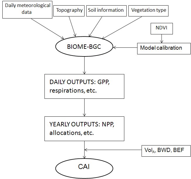
where BEF and BWD are the same as for eqn. 4 and SCA is the Stem C Allocation ratio of BIOME-BGC. These estimates were directly compared to the CAI measurements provided by INFC. A simplified scheme of the steps followed to estimate CAI is indicated in Fig. 2.
Fig. 2 - Simplified scheme of the modeling steps followed to obtain CAI estimates starting from the input data.
Both comparisons were made using the available aggregated data for the six forest types of Tuscany. The overall estimation accuracy over the six FTs was summarized by means of common statistics (i.e., correlation coefficient: r; root mean square error: RMSE; and mean bias error: MBE).
Results
Reproduction of IFT maximum volumes
The last column of Tab. 1 reports the average GPP values estimated for the six Tuscany FTs using BIOME-BGC with the original parameter settings. These GPPs generally follow the auto-ecological characteristics of the ecosystems: the lowest values are typical for mountain forests (FT 4 for broadleaves and FT 6 for conifers), while highest productions are found for lowland coniferous species. These GPPs are also in accordance with the measurements obtained by the eddy correlation technique ([17]).
As regards the carbon stocks estimates, they only partly follow these GPP patterns, due to the different respiration and allocation of the six forest types (Fig. 3). The potential volume estimates are generally higher than the maximum IFT measurements for most FTs. Small differences are found for FT 1 and FT 5, while for FT 2, FT 3, FT 4 and FT 6 the overestimation is very high.
Fig. 3 - Comparison between the reference volumes of the 6 FTs and the volumes estimated using the original and the new WPMFs.
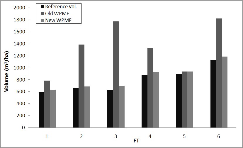
In almost all cases the new WPMFs identified by the current investigation (Tab. 2) are higher than the originals, which implies that woody biomass is accumulated in tree stems and coarse roots for a lower number of years. Exceptions are represented by FT 1, for which WPMF is slightly increased, and FT 5, for which WPMF is unvaried. These WPMF changes have direct consequences on the potential volumes simulated by BIOME-BGC (Fig. 3), while do not introduce significant differences in the predicted GPP (differences lower than 2%): the same is true for all respirations and LAI.
Tab. 2 - Definitive BIOME-BGC parameter settings. Only the model parameters changed with respect to default values are reported. The parameters controlling conductance reduction (leaf water potential and vapour pressure deficit) were reduced to 90% of the default values for the first three ecosystems and were left unchanged for the others. The last column reports the new WPMFs, which replace the default settings (0.005 1 yr-1) proposed by White et al. ([29]) for all forest types.
| Ecosystem type |
Maximum stomatal conductance (m s-1) |
Fraction of leaf N in Rubisco |
New WPMF (1 yr-1) |
|---|---|---|---|
| 1 | 0.0016 | 0.029 | 0.00625 |
| 2 | 0.0020 | 0.090 | 0.01 |
| 3 | 0.0023 | 0.078 | 0.0125 |
| 4 | 0.0045 | 0.090 | 0.01 |
| 5 | 0.0024 | 0.022 | 0.005 |
| 6 | 0.0032 | 0.027 | 0.01 |
Simulation of mean canopy covers and CAIs
The mean FCA and CAI values of the six forest types measured and estimated before and after the WPMF modification are shown in Fig. 4 and Fig. 5 together with relevant ground measurements. As regards FCA, the estimates obtained with the original WPMFs are much lower than the measurements for FT 1 and 2. In the other cases, minor but still significant differences are observed. The use of the new WPMFs strongly reduces the FCA underestimation for the first two FTs, and improves the estimation accuracy also for FT 4 and 6. Overall, this modification results in a notable increase of the correlation coefficient and in a significant reduction in the mean differences between the measured and estimated FCA values.
Fig. 4 - Comparison between actual forest cover (FCA) measured and estimated by the old and the new versions of BIOME-BGC. (*): significant correlation, P< 0.05.
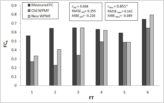
Fig. 5 - Comparison between current annual increments (CAI) measured and estimated by the old and the new versions of BIOME-BGC. (*): significant correlation, P< 0.05.
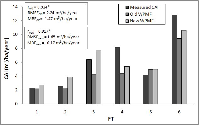
The comparison between measured and estimated CAIs provides similar results. The model with the original WPMFs strongly underestimates INFC CAIs for FT 3, 4 and 6. This problem is partly corrected by the use of the new WPMFs, with the highest improvement obtained for FT 3. As a consequence, the new WPMF settings lead to a substantial reduction of the mean errors: RMSEold = 2.24 m3 ha-1 year-1 and MBEold = -1.47 m3 ha-1 year-1 against RMSEnew = 1.65 m3 ha-1 year-1 and MBEnew = -0.17 m3 ha-1 year-1.
Discussion and conclusion
BIOME-BGC has been shown to be applicable to simulate the behaviour of a wide variety of forest ecosystems, both in terms of eco-physiological processes and accumulated carbon pools (e.g., [20], [17], etc.). Previous investigations in various European forest areas, however, indicated a model tendency to overestimate the stored carbon stocks (e.g., [20], [18]). Specifically, the maximum (potential) standing volumes simulated by the model are mostly higher than the volumes which can be actually found in most European forests. This implies errors in the simulation of net carbon accumulation processes which, in some cases, have been fixed empirically ([18]).
The current paper proposes a more sound approach to address this problem. This approach is based on the modification of a major parameter setting which controls carbon accumulation in the vegetation compartment, WPMF ([23]). The modification is performed by taking as reference values the maximum standing volumes derived from various forest inventories. This operation relies on the evidence that these inventories provide a large number of point measurements for each FT, which should guarantee the representativeness of the volumes found for production conditions close to the potential maxima and not significantly limited by occurred disturbances. The alternative use of parametric methods for the identification of these potential volumes (i.e., using standard deviation intervals from volume averages) has been found to be currently unfeasible, due to the marked non-normality of the volume statistical distributions.
The application of the current method yields new WPMFs which are not descriptive of the ages reachable by the six forest types in all conditions. In fact, the WPMFs identified are related to the average turn-over times which would characterize the existing forests in the absence of disturbing factors. Consequently, these WPMFs are dependent on local environmental factors (fertility, climate, growth form, etc.), and are not directly exportable to all other cases.
As expected, the use of new WPMFs does not modify the original LAI, GPP and respiration estimates but leads to substantial changes in accumulated stem carbon. The new volume averages of the six forest types are mostly lower than the original values and more consistent than these with the estimates provided by different sources ([6], [7]).
The WPMF modification results in a marked improvement in the reproduction of the carbon stocks stored in the woody ecosystem compartment. This improvement is decisive in enhancing the assessment of NVA and FCA. As a consequence, the modification implies a substantial enhancement in the estimation of net production processes (i.e., woody NPP).
These results are particularly relevant when considering that all model simulations have been performed over forests which are very heterogeneous due to the variable climate and site factors and to the different management practices which characterize Tuscany environments. It can therefore be concluded that the use of the new BIOME-BGC versions can significantly enhance the capacity of the modeling strategy to simulate carbon stocks and fluxes across a variety of Mediterranean forest ecosystems.
Acknowledgements
The work was partially carried out under the C_FORSAT project “Modelling the carbon sink in Italian forest ecosystems using ancillary data, remote sensing data and productivity models” (national coordinator: Prof. G. Chirici), funded by the FIRB2008 program of the Italian Ministry of University and Research (RBFR08LM04).
The authors thank Dr. M. Moriondo, Dr. L. Fibbi and Prof. M. Bindi for their assistance in the calibration and application of BIOME-BGC in Tuscany, and Prof. P. Corona for his precious comments on the subject of the paper.
References
Gscholar
Gscholar
Gscholar
Gscholar
Gscholar
Gscholar
Gscholar
Gscholar
Gscholar
Gscholar
Gscholar
CrossRef | Gscholar
Gscholar
Authors’ Info
Authors’ Affiliation
EcoGeoFor - Università del Molise, Contrada Fonte Lappone snc, I-86090 Pesche (IS - Italy)
Corresponding author
Paper Info
Citation
Chiesi M, Chirici G, Barbati A, Salvati R, Maselli F (2011). Use of BIOME-BGG to simulate Mediterranean forest carbon stocks. iForest 4: 121-127. - doi: 10.3832/ifor0561-004
Paper history
Received: Jul 12, 2010
Accepted: Jan 22, 2011
First online: Jun 01, 2011
Publication Date: Jun 01, 2011
Publication Time: 4.33 months
Copyright Information
© SISEF - The Italian Society of Silviculture and Forest Ecology 2011
Open Access
This article is distributed under the terms of the Creative Commons Attribution-Non Commercial 4.0 International (https://creativecommons.org/licenses/by-nc/4.0/), which permits unrestricted use, distribution, and reproduction in any medium, provided you give appropriate credit to the original author(s) and the source, provide a link to the Creative Commons license, and indicate if changes were made.

Web Metrics
Breakdown by View Type
Article Usage
Total Article Views: 60258
(from publication date up to now)
Breakdown by View Type
HTML Page Views: 50067
Abstract Page Views: 3760
PDF Downloads: 4430
Citation/Reference Downloads: 26
XML Downloads: 1975
Web Metrics
Days since publication: 5521
Overall contacts: 60258
Avg. contacts per week: 76.40
Article Citations
Article citations are based on data periodically collected from the Clarivate Web of Science web site
(last update: Mar 2025)
Total number of cites (since 2011): 11
Average cites per year: 0.73
Publication Metrics
by Dimensions ©
Articles citing this article
List of the papers citing this article based on CrossRef Cited-by.
Related Contents
iForest Similar Articles
Commentaries & Perspectives
Reply: “Use of BIOME-BGC to simulate Mediterranean forest carbon stocks”
vol. 4, pp. 249 (online: 03 November 2011)
Research Articles
Simplified methods to inventory the current annual increment of forest standing volume
vol. 5, pp. 276-282 (online: 17 December 2012)
Research Articles
Assessing most relevant factors to simulate current annual increments of beech forests in Italy
vol. 7, pp. 115-122 (online: 31 December 2013)
Research Articles
Modelling the carbon budget of intensive forest monitoring sites in Germany using the simulation model BIOME-BGC
vol. 2, pp. 7-10 (online: 21 January 2009)
Commentaries & Perspectives
Comment on Chiesi et al. (2011): “Use of BIOME-BGC to simulate Mediterranean forest carbon stocks”
vol. 4, pp. 248 (online: 03 November 2011)
Research Articles
Allometric relationships for predicting the stem volume in a Dalbergia sissoo Roxb. plantation in Bangladesh
vol. 3, pp. 153-158 (online: 15 November 2010)
Research Articles
Modeling compatible taper and stem volume of pure Scots pine stands in Northeastern Turkey
vol. 16, pp. 38-46 (online: 22 January 2023)
Research Articles
Use of BIOME-BGC to simulate water and carbon fluxes within Mediterranean macchia
vol. 5, pp. 38-43 (online: 02 April 2012)
Research Articles
Scots pine’s capacity to adapt to climate change in hemi-boreal forests in relation to dominating tree increment and site condition
vol. 14, pp. 473-482 (online: 18 October 2021)
Research Articles
Incorporating management history into forest growth modelling
vol. 4, pp. 212-217 (online: 03 November 2011)
iForest Database Search
Search By Author
Search By Keyword
Google Scholar Search
Citing Articles
Search By Author
Search By Keywords
PubMed Search
Search By Author
Search By Keyword


