Total tree height predictions via parametric and artificial neural network modeling approaches
iForest - Biogeosciences and Forestry, Volume 15, Issue 2, Pages 95-105 (2022)
doi: https://doi.org/10.3832/ifor3990-015
Published: Mar 21, 2022 - Copyright © 2022 SISEF
Research Articles
Abstract
Height-diameter relationships are of critical importance in tree and stand volume estimation. Stand description, site quality determination and appropriate forest management decisions originate from reliable stem height predictions. In this work, the predictive performances of height-diameter models developed for Taurus cedar (Cedrus libani A. Rich.) plantations in the Western Mediterranean Region of Turkey were investigated. Parametric modeling methods such as fixed-effects, calibrated fixed-effects, and calibrated mixed-effects were evaluated. Furthermore, in an effort to come up with more reliable stem-height prediction models, artificial neural networks were employed using two different modeling algorithms: the Levenberg-Marquardt and the resilient back-propagation. Considering the prediction behavior of each respective modeling strategy, while using a new validation data set, the mixed-effects model with calibration using 3 trees for each plot appeared to be a reliable alternative to other standard modeling approaches based on evaluation statistics regarding the predictions of tree heights. Regarding the results for the remaining models, the resilient propagation algorithm provided more accurate predictions of tree stem height and thus it is proposed as a reliable alternative to pre-existing modeling methodologies.
Keywords
Tree Height Model Prediction, Generalized Models, Mixed-Effects Models, Levenberg-Marquardt Algorithm, Resilient Propagation
Introduction
Natural forest areas have continued to decline in the last 30 years while plantations have increased in the same timeframe, now comprising some 7% of the global forest area. Plantations are of great importance in economic and ecological terms. Thus, robust and reliable information on the growth and development characteristics of these species are essential in order to sustainably manage plantations and determine the success of afforestation efforts. Diameter at breast height (d) of trees and total tree-bole height (h) are two basic commonly used parameters in forest inventory, planning and management of plantations. These parameters are fundamental variables in several forest practices such as prediction of standing yield, growth projection, carbon accounting, identification of stand structural diversity, determination of the extent of damage in forest or stands, and to estimate missing tree heights ([15], [1]).
In forest management applications or field inventories, d in trees can be measured rapidly and precisely, while h is costly, more time consuming, and challenging to measure ([45], [66], [53]). It is also known that there is a strong correlation between d and h in the stem of trees. Because of this, models can be created to discover the relationship between d and h based on the tree diameter at breast height and the total stem height of trees that are measured. Ultimately, these models are used to estimate the height of any tree in the stand with unknown height ([60], [35]).
There are many studies describing tree height estimation and prediction models, mainly using well-known classical modeling techniques, such as non-linear regression models ([11], [31]) and Bayesian modeling ([81]), using in most cases allometric models. Further research evaluating more recent and promising modeling methods such as techniques based on the artificial intelligence are warranted to improve efficacy. Previous research on height-diameter (h-d) modeling of cedar plantations in Turkey was conducted by Catal ([9]), although it was based on a limited number of traditional h-d models, without further investigation of the potential efficiency of other modeling approaches.
Generally, h-d models may be simple or generalized. Simple models utilize d to calculate h, as the relationship between the two variables is well-known ([6]). The limitation with simple models, however, is the large sampling effort required ([24]). In contrast, the correlation between d and h (total height) varies among species and can be influenced by stand-specific variables such as stand structure and site productivity ([38]). Models that include measures of stand structure, site productivity and tree social position are commonly referred to as generalized h-d (GM) models. Mehtätalo et al. ([44]) used fixed-effects (FE) and generalized mixed-effects (ME) modeling techniques to show differences between marginal and plot-specific h-d relationships, in a range of different geographical/ecological regions and tree species. The use of additional stand-level variables was previously shown to improve tree height estimates ([75], [38]). For example, Newton & Amponsah ([48]) used dominant height (H0) within a stand to estimate stand-level competition.
Since the estimation and prediction of tree heights are crucial in tree growth and tree volume prediction, alternative and accepted modeling techniques exist such as the generalized, FE and ME models, and artificial neural network modeling techniques, that may be useful in modeling the relationship between h-d and reducing the measurement efforts on the ground. The most basic ([28], [56], [68]) and generalized h-d models ([25], [1], [75], [14], [38], [82], [53]) are available for many tree species. Most research has focused on mixed-models to understand h-d relationships ([7], [66], [38], [50], [53], [24], [25], [44], [2], [6]). In Turkey, h-d equations were developed for some tree species at regional scale ([16], [51], [10]).
Taurus cedar (Cedrus libani A. Rich.) natural range includes the Taurus Mountains of Turkey, where it is an ecologically and economically important component of the forest ecosystems ([5]). The most recent inventory data show that cedar covers an area of approximately 463,521 ha in Turkey, with a total growing stock of 27.4 million m3 ([23]). It is not only an important resource of raw material for the forest product industry, but it also fulfils critical ecological tasks including the reduction of soil erosion and the conservation of water resources, the mitigation of the adverse impacts of climate change, and is essential in the maintenance of biological diversity in Turkey. It has moderate soil requirements and is tolerant to extremes of temperature and drought in summer and to cold temperatures in winter ([61]); therefore, C. libani has great potential for afforestation, especially in areas with semi-arid climates. Given that 35% of Turkey’s territory has semi-arid climate, cedar is a critical tree species for use in afforestation. As of 2000, an area of approximately 110,000 ha was re-afforested with cedar ([32]). However, there is still relatively little information concerning the growth of Taurus cedar plantation compared with the quantity of information available for natural cedar stands. H-d relationship is one of the most important components of growth and yield models for sustainable management of Taurus cedar plantations. Moreover, to our best knowledge, h-d generalized mixed-effects model has not been developed for Taurus cedar plantations.
Until now, the use of artificial neural networks (ANNs) in forest modeling has led to the conclusion that they can be considered as significant alternative techniques for many characteristics of trees growth compared to classical modeling methods, both in classification tasks ([65], [40], [13]), and for estimation and prediction problems ([36], [67], [58], [52], [18], [47], [73], [80], [69]). Specifically, artificial intelligence was successfully implemented to the development of total tree height models as well ([39], [16], [50], [76], [71], [19]). The majority of the ANN modeling studies employed multilayer perceptron architecture combined by the standard backpropagation algorithm.
The incentive for developing an artificial neural network modeling approach in the present work was that ANNs can discover and thus automatically model the relationships underlying input and output variables, a property reflected in the connection weights of the network. Instead, traditional approaches, such as the widely accepted generalized, fixed and mixed-effects modeling methods, require certain assumptions about the form of a fitting function which must be specified in advance, introducing limitations that mainly impact model applicability to different scenarios. In contrast, an ANN model is trained to find this relationship, thus fitting complex nonlinear models. In addition, given that ANNs provide resilience to outliers, the techniques generally perform well where there are missing or inaccurate data; this problem is typically found in forest-data measurements which require substantial effort in-the-field, increasing proneness to errors. Furthermore, this generalization ability enables ANN models to generate reliable predictions with new data sets. ANN modeling techniques, therefore, can overcome problems in basic data gathered in the forest, including nonlinear relationships, multicollinearity, heteroscedasticity, outliers and noise. Although ANNs may suffer from over-fitting of data, this problem can be avoided by selecting a suitable training architecture followed by testing and validation.
The objective of this work was to compare the effectiveness of different modeling approaches in providing accurate predictions of total stem height of C. libani plantations of Turkey. After developing the ANN models, validation was carried out using simple measurements from the forest environment, such as d. Variability between sampling plots was included in the models by recording dominant heights (H0) and diameters (D0) of each sample plot. The adjusted fixed-and mixed-effects models, after being localized using calibration data from one to three sample cedar trees were compared against the prediction abilities of the novel ANN models. For this purpose, two different learning algorithms, that have shown significant ability to cope the known disadvantages and limitations of the most used standard backpropagation learning algorithm ([79]), i.e., the resilient propagation (RPANN) and the Levenberg-Marquardt (LMANN), were applied as innovative modeling strategies in forest model building, with the aim of optimizing the learning process and better exploting the information in real data measurements originating from the forests.
Materials and methods
Site description
Data used for development of models were gathered in cedar plantations. Sample plots were in the Isparta Regional Directorate of Forestry, which includes the Isparta and Burdur provinces (south-western Turkey), at an elevation between 1000 to 1600 m a.s.l. Climate in this region is characterized as transitional from the Mediterranean to continental climate. Annual precipitation varies between 426 to 814 mm, while annual mean temperature ranges from 11.9 to 13.2 °C ([46]). The bedrock of the study site is composed of sedimentary rock including limestone, sandstone, and claystone.
Data collection
To determine diameter-height associations, data were collected from 30 sampling plots randomly distributed among Taurus cedar plantations in Isparta and Burdur Forest Regions. Sample plots were selected to represent a range of age classes, site conditions, and densities for the species in the Mediterranean Region of Turkey. Plot size varied between 270 to 540 m2, depending on density, with a minimum of 30 trees per plot. The age of the sampling plots varied from 17 to 35. Two perpendicular over-bark diameters (di) were measured with a precision of 0.1 cm and averaged to find actual diameter (d, cm) for each tree. A Blume-Leiss hypsometer was used to obtain total heights with precision of 0.5 m. Depending on plot size, dominant heights (H0) and diameters (D0) were obtained as the average heights and diameters of the 100 trees with the thickest diameter at breast height (d) per hectare.
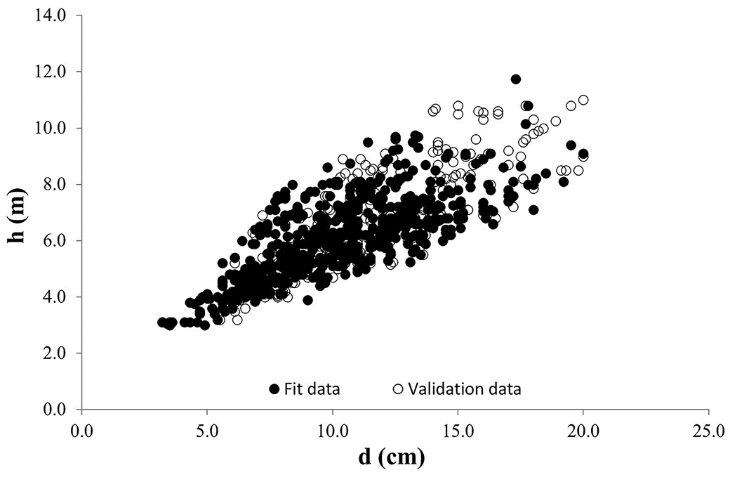
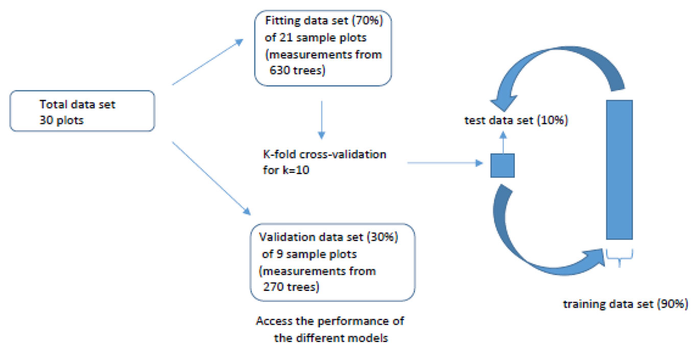
The available Cedar data set was randomly split into two groups; some 21 sample plots (70% of all plots) were randomly selected for the model fitting while the remaining 9 sample plots (30% of all plots) were used for evaluating the models’ performance on this new data set (Tab. 1). The basic descriptive statistics for the dataset used has been given in Tab. 1and illustrated in Fig. 1.
Tab. 1 - Summary statistics for the fitting and the validation data sets. (d): diameter at breast height (1.3 m above the ground); (h): total tree height; (H0): dominant height; (D0): dominant diameter; (G): basal area per hectare; (dm): mean diameter; (hm): mean height; (Dg): quadratic mean diameter; (SD): standard deviation.
| Variable | Fitting data (70%) (630 trees in 21 plots) |
Validation data (30%) (270 trees in 9 plots) |
||||||
|---|---|---|---|---|---|---|---|---|
| Mean | Min | Max | SD | Mean | Min | Max | SD | |
| d (cm) | 10.31 | 3.20 | 20.00 | 3.12 | 11.37 | 5.40 | 20.00 | 3.50 |
| h (m) | 6.12 | 3.00 | 11.75 | 1.42 | 6.66 | 3.20 | 11.00 | 1.81 |
| Age (years) | 26.00 | 17.00 | 35.00 | 6.30 | 31.00 | 23.00 | 35.00 | 4.70 |
| D0 (cm) | 13.96 | 9.72 | 18.30 | 2.38 | 14.86 | 7.82 | 19.24 | 3.49 |
| H0(m) | 7.51 | 5.44 | 10.02 | 1.21 | 8.30 | 5.66 | 10.65 | 1.67 |
| G (m2 ha-1) | 30.30 | 12.75 | 50.70 | 10.86 | 36.96 | 12.01 | 58.25 | 15.02 |
| dm(cm) | 10.29 | 6.68 | 13.53 | 2.02 | 11.35 | 6.74 | 14.64 | 2.51 |
| hm(m) | 6.10 | 4.31 | 7.93 | 1.03 | 6.66 | 4.50 | 8.65 | 1.37 |
| Dg(cm) | 10.57 | 6.98 | 13.92 | 2.08 | 11.60 | 6.77 | 14.92 | 2.59 |
Fig. 1 - Scatter plot of total height (h) against diameter at breast height (d) for cedar pine trees for both fitting and validation data sets.
Generalized height-diameter models (GM)
Twenty-one generalized height-diameter models selected from earlier studies were evaluated using non-linear least squares (NLS - [14], [12]). These models included different stand-level variables such as H0, D0, and quadratic mean diameter, to represent the variation between forest stands.
Fixed-effects model (FE)
A large number of nonlinear model forms with two and three parameters were evaluated for cedar plantations, including those noticed by Huang et al. ([28]) and Lei et al. ([35]) as Curtis, Weibull, Exponential, Chapman-Richards, Gompertz, Schnute, and Korf-Lundgvist. The NLS were fitted to the datasets to determine the most appropriate model for cedar plantations. To evaluate the prediction accuracy of the models, statistical and graphical evaluations were used. Of the models assessed, predictive capability of the Chapman-Richards appeared best to model height-diameter relationships in cedar plantations (eqn. 1):
where hij is the total tree height (m) of the j-th tree in the i-th plot, dij is the diameter (cm), and β1- β3 are model parameters.
To calibrate the FE model, a correction factor k* (eqn. 2) suggested by Temesgen et al. ([70]) was used. Temesgen et al. ([70]) indicated that when the heights of a subsample of nim trees from the i-th stand is known, the predicted heights of the remaining trees from the same stand can be calibrated (eqn. 2):
where hat{h}hi is the predicted height from the FE model (eqn. 1), and hij is the observed value.
The predicted values of height (tilde{h}) for the remaining trees in the same stand can be calculated as follows (eqn. 3):
The influence of the correction factor on the prediction accuracy of a nonlinear FE model was also investigated.
Nonlinear mixed-effects model (ME)
In the ME model structure, parameters of eqn. 1 comprise the plot-specific random-effect parameters and the population level fixed-effect parameters that are common to all trees. In matrix notation, eqn. 1 can be represented as (eqn. 4):
where yi = [hi1, hi2, …, hin]T, di = [di1, di2, …, din]T, εi = [εi1, εi2, …, εin]T, ni is the sample size for tree height values in plot i, and ui and b and are column vectors representing random- and fixed-effects parameters, respectively; εi ~N(0,R) and ui ~N(0,D), where R and D are diagonal matrices. Additionally, it is assumed that ui and εi are independent. SAS procedure NLMIXED ([63]) was used to obtain the parameters of nonlinear ME models (eqn. 4).
The first-order Taylor series expansion can be used to obtain the random-effect parameters ui for the i-th plot ([27], [45] - eqn. 5):
where ûik is an estimate of the random-effect parameters for plot i at the k-th iteration, hat{D} is an estimate of D, the variance-covariance matrix for ui, and Zi is (eqn. 6):
hat{R} is an estimate of R, the variance-covariance matrix for εi, yi is the m × 1 vector of observed tree heights, and m is the number of tree height measurements used to localize the height growth model.
Estimating ui requires an iterative process. In eqn. 5, a null starting value (ûi0=0) was used and repeatedly updated until the absolute difference between ûik and ûik+1 was smaller than a predetermined tolerance limit. For the random effects, the outcome is the approximated empirical best linear unbiased predictor (EBLUP).
ANN models
The most significant advantage of an ANN model is that it is trained from measured data without the need to add further information. That is, after the fitting of the system with the available ground-truth data, the ANN model automatically discovers the existing dependencies, and finally produces a trained model. On the other hand, the net topology, the learning algorithms used, and the learning constrains are specified by the modeler.
Levenberg-Marquardt artificial neural network model (LMANN)
The Levenberg-Marquardt (LM) algorithm was selected for application in the multilayer perceptron learning of ANN ([37], [42]). Past studies showed that the LM algorithm has the ability, on the one hand, to cope with known disadvantages and limitations of the standard backpropagation learning algorithm, such as slow convergence, much off-line training requirements, instability, trapped at local minima ([3], [77], [64], [79]); on the other hand, LM algorithm have showed significant ability on the prediction of environmental variables ([78], [17], [83], [54]).
A detailed description of how the Levenberg-Marquardt algorithm is embedded to neural network training can be found in Hagan & Menhaj ([26]). Concisely, the Hessian matrix (Hm) approximation is introduced by the LM algorithm as ([54] - eqn. 7):
where I is the identity matrix, J is the Jacobian matrix, and μ is the combination coefficient.
The update rule of the LM algorithm is wt+1 = wt - (Hm)-1 JTe, where w are the weights, and e are the biases. The efficiency and convergence of the LMANN models are very sensitive to the configuration of the coefficient value (μ) of eqn. 7. As the value becomes larger, the more weight is given to gradient descent learning with a small step size. The smaller it is, the more weight is given to large step sizes. For μ equal to zero, the algorithm turns to the Gauss-Newton method.
Resilient propagation artificial neural network model (RPANN)
Resilient propagation, known as Rprob, is a neural network algorithm which was fully described by Riedmiller & Braun ([59]) and successfully used ([62], [21]), so that known disadvantages of the standard back-propagation algorithm can be overcome. The back-propagation algorithm has known drawbacks, due to elementary learning processes. The main problems of the learning phase include slow convergence resulting from small changes in weights, and the neural network weights trapping around local optima.
Rprob mainly refers to the gradient direction. The algorithm calculates a delta value (Δij) for each weight that increases when the gradient does not change sign under the prerequisite that the system works on the right direction, or decreases when the gradient does change sign. The learning rule used to calculate delta value which improves the change of the network weights is the following ([59] - eqn. 8):
where 0 < η- < 1 < η+.
Finally, the new weight value wtij between i and j neurons in two consecutive layers on the (t-1) is given by (eqn. 9):
Aspects of ANN model training
In geotechnical engineering, the selection of the proper input variables for ANN model building is usually based on a priori knowledge of the physical problem ([41]). In order to construct a reliable model for total stem height prediction, the sensitivity analysis was used to choose the proper input layer nodes of the ANNs. The analysis was performed on the available variables measured in the field (Tab. 1), that were selected in advance due to the physical problem ([8]).
To avoid overfitting and undertraining of the network in reaching the best possible training efficiency of the model, the training process was initiated with the smallest possible network and no hidden nodes. Then the construction of the model continued by adding any necessary hidden nodes in order the network learning to be completed. Finally, the architecture is reached to an end, when the agreement obtained between ANN model predictions and targets can be considered as satisfactory.
Overfitting avoidance of the ANN models led to acceptable generalization ability of the models. For this reason, the k-fold cross validation resampling method with k=10 was applied ([49], [43]) to both training and testing data sets ([34]), due to its efficiency and easiness to apply. This procedure was not applied in regression model building, where there is little to be gained by separating data into parts ([30]). As described above, the whole data set was randomly divided into two parts. The fitting data set was used for the construction of all different types of models. The validation data set was used only for the evaluation of the predictive capability of all constructed models.
Due to the fact that the ANN model error value is strongly affected by the number of the weights, the credibility and the generalization capability of the model was determined through the mean error rate on the cross-validation examples, and the validation data set, respectively (Fig. 2).
Fig. 2 - The 10-fold cross validation division for the ANN models construction.
As mentioned above, the efficiency and convergence of training of the LMANN models significantly depends on the proper value selection for the combination coefficient (μ in eqn. 7). The initial value of μ was set to 0.001 ([17]) and the final value that led to the lowest sum of square errors model value was found equal to 1.00e-07.
Similar to the LMANN models, training of RPANN models is very sensitive to the value of delta rule Δij(t) (eqn. 8), which is responsible for the sign (positive or negative) of the gradient to show the direction of the adjustment weight. Through this process the iteration of learning stops when the error target is reached. The initial delta value was 0.07, with increment steps of 1.2 and decrease steps of 0.5.
The architecture of both the LMANN and RPANN algorithms finalized after the detection of the correct number of nodes in the hidden layer. This final number was obtained during a trial-and-error process: the process began with one hidden node and was repeated until the desired target error value was reached. During the trial-and-error process, selection of the correct combination of transfer functions was made. The combination of functions that provided the optimal behavior of both the ANN models was: (i) the hyperbolic tangent transfer function (tansig) to transfer knowledge from the input layer to the hidden layer; and (ii) the linear activation function (purelin), transferring information from the hidden layer to the output layer ([20]). The ANN models were constructed using the neural network toolbox of the MATLAB software ver. R2017a ([4]) developed by The Math Works™ Inc.
Evaluation
The evaluation of the different modeling approaches (i) Generalized Model (GM), (ii) non-calibrated fixed-effects model [FE(0)], (iii) calibrated fixed-effect model [FE(1-3)], (iv) calibrated mixed-effects model [ME (1-3)], (v) LMANN, and (vi) RPANN techniques, was made using the mean difference (MD, m), the mean absolute difference (MAD, m), the fit index (FI) and the root square mean error (RSME), which were calculated as follows (eqn. 10 to eqn. 13):
where n is number of plots, ni is number of tree height values for plot i, hij and hat{h}ij are measured and predicted heights, respectively, and bar{h}i is mean height of hij for plot i.
It is worth noting, that the adjusted FE and the calibrated ME models’ parameters were “localized” by the use of a number of sampled heights in each plot. Trincado et al. ([72]) recommended that the number of tree heights measured in each plot ranged from one to three. Finally, to compare and evaluate the generalization ability of the constructed models by the different modeling approaches, the above metrics were computed for the validation data set as well ([53], [6]).
Results
Parametric modeling approaches (generalized models, fixed-and mixed-effects models)
Twenty-one GM models were fitted using the NLS method with the fitting data set, while the predictive capability of the models was evaluated using the validation data set. The final GM model ([33]) including D0 and H0 as additional independent variables, was (eqn. 14):
The model given in eqn. 14 and its modified forms was successfully used by many authors (e.g., [14]). H0 was the most important contributor among stand level variables since it can allow a plot-level adaptation related to many factors, such as genetics, topography, silvicultural regime, and environment ([29]). Further, the accuracy of h-d models can be improved by the incorporation of D0 and H0 as covariates ([14], [57]).
Tab. 2 - Fit statistics for eqn. 1 for different combinations of random parameters.
| Random Parameters | AIC (smaller is better) | BIC (smaller is better) |
|---|---|---|
| None (Fixed-effects) | 2503 | 2522 |
| β 1 | 1617 | 1624 |
| β 2 | 1821 | 1828 |
| β 3 | 1605 | 1612 |
| β1 and β2 | 1540 | 1550 |
| β1 and β3 | 1539 | 1548 |
| β2 and β3 | 1714 | 1724 |
| β1, β2 and β3 | 1656 | 1670 |
A series of parameters from eqn. 1 was implemented (Tab. 2). Model (1) with random components β1 and β3 resulted in the lowest values for both Akaike’s (AIC) and Bayesian (BIC) information criteria. The final ME model was (eqn. 15):
where u1 and u2 are random parameters. Parameter estimates were obtained using the fitting data set for the best models (GM, FE and ME models) and are given in Tab. 3.
Tab. 3 - Parameter estimates and standard errors (in parentheses) for the fixed- and mixed-effects regression models. (σ2): residual variance of the model; (σ2u1): variance of the random-effect u1; (σ2u2): variance of the random-effect u2; (σ2u1 u2): covariance of the random-effects u1 and u2.
| Parameter estimates | Generalized Model | Fixed-effects | Mixed-effects |
|---|---|---|---|
| β 1 | -6.9087 (0.5670) | 7.8237 (0.6187) | 24.7062 (11.3829) |
| β 2 | -0.0294 (0.0045) | 0.1348 (0.0315) | 0.0159 (0.0113) |
| β 3 | - | 1.5604 (0.2998) | 0.8643 (0.0750) |
| σ2 | - | 0.8311 (0.0468) | 0.2216 (0.0129) |
| σ2u1 | - | - | 73.9740 (113.22) |
| σ2u2 | - | - | 0.0448 (0.0176) |
| σ2u1 u2 | - | - | 1.6671 (1.3800) |
According to the predictions, the marginal non-calibrated fixed-effects (FE) response model gave more unsuccessful outcomes, when random parameters of the mixed models were zero and prior height information was not available for model calibration for both datasets (Tab. 4).
Tab. 4 - Fit statistics for the constructed basic h-d mixed-model, generalized h-d model and artificial neural network models (LMANN and RPANN) for (a) the fitting dataset, (b) the validation data sets, and (c) the calibrated adjusted fixed and mixed models, using 1, 2, and 3 sampled trees for calibration. (§): denote the best method for cedar plantations; (*): for p-value <0.05, the null hypothesis (Ho: μ1=μ2) was rejected.
| Dataset | Model | Type | RMSE | FI | MD/two tailed p-value* |
MAD |
|---|---|---|---|---|---|---|
| (a) Fitting data set (630 trees in 21 plots) |
LMANN: 3-2-1 | ANN | 0.5512 | 0.8241 | -0.0407494 | 0.4306 |
| RPANN: 3-2-1 | ANN | 0.5387 § | 0.8353 | 0.0074/0.729 | 0.4155 § | |
| Chapman-Richards (eqn. 1) | Fixed | 0.9116 | 0.5912 | -0.0019833 | 0.7088 | |
| Chapman-Richards (eqn. 15) | Mixed | 0.6316 | 0.8059 | 0.1905/0.000 | 0.4684 | |
| Krumland & Wensel (eqn. 14) | Generalized | 0.5677 | 0.8422 | -0.7526316 | 0.4299 | |
| (b) Validation data set (270 trees in 9 plots) |
LMANN: 3-2-1 | ANN | 0.6839 | 0.8 | -0.1138 | 0.5673 |
| RPANN: 3-2-1 | ANN | 0.6671 § | 0.8176 | -0.0995 § | 0.55 § | |
| Chapman-Richards (eqn. 1) | Fixed [F(0)] | 1.1401 | 0.6017 | 0.2101 | 0.8943 | |
| Krumland & Wensel (eqn. 14) | Generalized (GM) | 0.721 | 0.7825 | -0.2272 | 0.5985 | |
| (c) Validation data (270 trees in 9 plots) after using localization |
Chapman-Richards (eqn. 3) | Fixed-Calibrated, FE(1) | 0.8759 | 0.7649 | 0.3114 | 0.6417 |
| Chapman-Richards (eqn. 3) | Fixed-Calibrated, FE(2) | 0.7427 | 0.831 | -0.1683 | 0.5937 | |
| Chapman-Richards (eqn. 3) | Fixed-Calibrated, FE(3) | 0.7348 | 0.8346 | -0.1778 | 0.5809 | |
| Chapman-Richards (eqn. 15) | Mixed-Calibrated ME(1) | 0.7573 | 0.8243 | 0.2129 | 0.5798 | |
| Chapman-Richards (eqn. 15) | Mixed- Calibrated ME(2) | 0.6799 | 0.8585 | -0.1335 § | 0.5377 | |
| Chapman-Richards (eqn. 15) | Mixed-Calibrated ME(3) | 0.6773 § | 0.8594 § | -0.1523 | 0.5242 § |
Artificial neural network modeling approaches
ANN models used a three-layer architecture that included: (i) one input layer with three variables (diameter at breast height, d; dominant height, H0; and dominant diameter, D0). Sensitivity analysis was performed using the available variables listed in Tab. 1. The three variables given above had significant entry on the target variable configuration, with a value of error ratio higher than one; (ii) one output layer with one target variable (total tree stem height, h) specified by the physical problem; and (iii) one hidden layer, comprising the proper number of hidden nodes specified by the network learning.
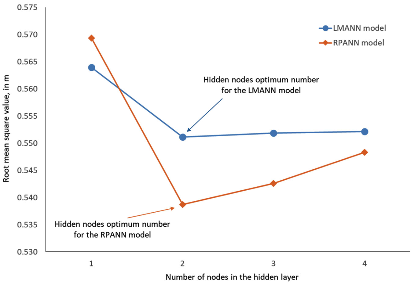
Using the LM algorithm for ANN model learning, the LMANN showing the best adaptation to the fitting data set was 3-2-1/0.5512, i.e., the specific model included a single input layer with the input nodes d, H0 and D0, one hidden layer with two hidden nodes and an output layer with one node (h), with RMSE equal to 0.5512. Using the RP algorithm for ANN model learning, the RPANN showing the best adaptation to the fitting data set was the 3-2-1/0.5387 model, i.e., the specific model comprised one input layer with input variables d, Ho and Do, a single output layer with output node h as in LMANN models building and, between these layers, a single hidden layer with two hidden nodes resulted from the trial-and-error process. The RMSE was 0.5387. For both ANN algorithms, the optimum number of hidden nodes was determined following examination of different numbers of nodes. The optimum values were selected as those leading to the best learning of the ANN models, with the smallest RMSE value (Fig. 3).
Fig. 3 - Optimum number of nodes in the hidden layer for the LMANN and RPANN models.
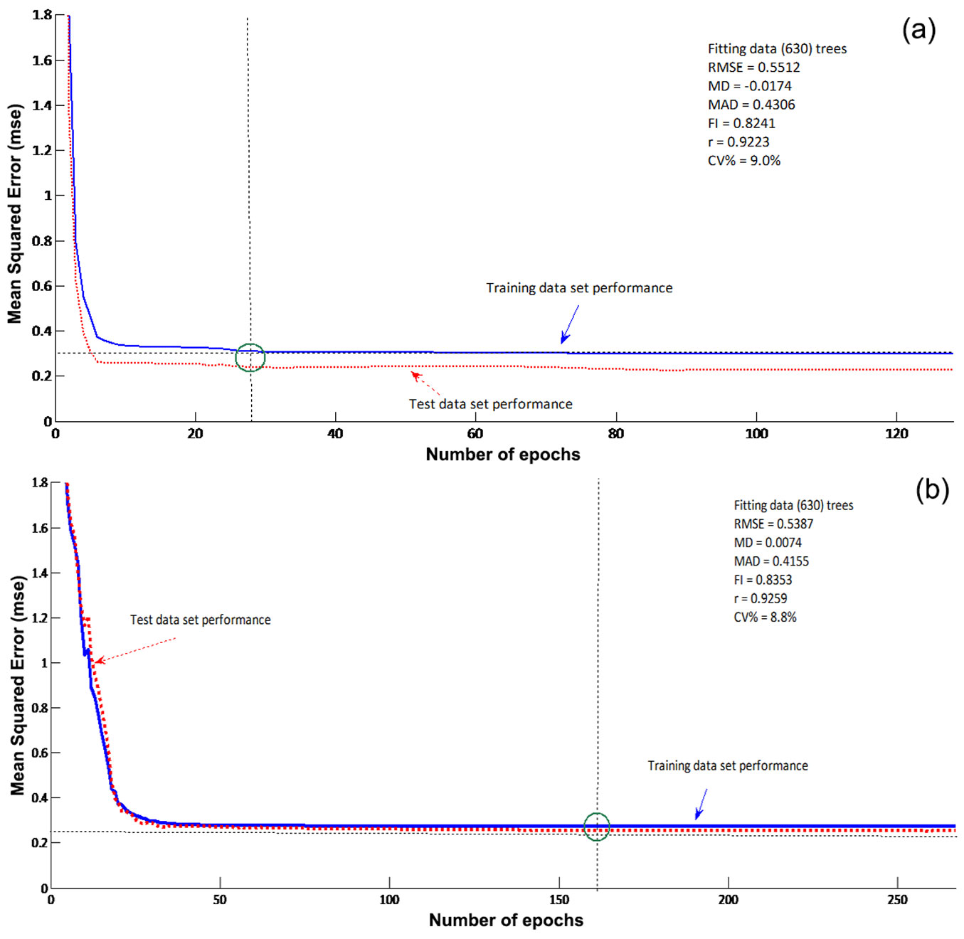
The k=10 cross validation method applied during the learning using the fitting data set for both ANN algorithms for training and testing in the construction phase, ensured the absence of overfitting and increased the ability of the ANNs to generalize. Both networks were trained for as many epochs as required for the models to reach the minimum MSE value (Fig. 4). As shown in Fig. 4, the estimated errors for the training and the test data sets were not significantly different for either ANN model, which indicated the absence of overfitting. The LMANN was stopped after 200 training interactions (epochs) as no influential reduction of the MSE value occurred after 28 epochs, while the RPANN was trained for 500 interactions as there was no influential reduction in MSE after 167 epochs (Fig. 4).
Fig. 4 - LMANN (a) and RPANN (b) models’ training and test performance for the best case of two hidden nodes in the hidden layer, using the fitting data set.
Evaluation of the different modeling approaches
A synopsis of the evaluation statistics calculated with the fitting and validation data sets using the different modeling approaches is given in Tab. 4. The best outcomes among the GM models are reported in Tab. 4. Comparing the MD, MAD, RMSE, and FI values for the fitting data set, both the RPANN and the LMANN models gave the best results (Tab. 4). Further, in order to enrich the conclusions derived from the results for the constructed models using the fitting data set, where the total height approximately normally distributed, the t-paired test was applied. The two-tailed p-values of the test were <0.05 for both the LMANN and the RPANN constructed models, suggesting that there is no mean difference between the observed and the estimated height values. The same conclusion can be derived for both the fixed-effects (FE) Chapman-Richards model (eqn. 1) and the generalized Krumland & Wensel (eqn. 14) model, while the mean error of mixed-effects model (eqn. 14) was found significant (p<0.05) for the fitting data set.
The accuracy of the estimated results from the ANN models was examined further by analyzing the correlation between the observed h values and their predictions from the models ([22]). The Pearson’s correlation coefficient (r) was computed as the ratio between the covariance of the observed heights and the height predictions by the constructed models. The LMANN model’s estimations gave r = 0.9223, while for the RPANN model gave r = 0.9259, indicating a high accordance between observed and predicted values. The variability of the estimation errors (CV% = (RMSE/hat{h} · 100) in relation to the mean of the total tree height for the fitting data set was 9.00% and 8.80% of the mean height for the LMANN and the RPANN models, respectively. The reliability and the predictive capabilities of both ANN models was also examined based on the validation data set taken from 270 trees in 9 plots in the same forest areas. The LMANN model predicted an r value of 0.9318 with a CV% of 10.27%, while the r value for the RPANN model was 0.9336, with a CV% of 10.02%. According to the validation data set, the Chapman-Richards mixed-calibrated model using three trees for calibration showed the next best predictive capabilities, with CV% equals to 10.17% and r = 0.9309, while the non-calibrated generalized model of Krumland & Wensel ([33]) gave similar results as compared to Chapman-Richards mixed-calibrated model, with CV% equals to 10.83% and r = 0.9269. Finally, the Chapman-Richards fixed-model produced the poorest results for the validation data set with CV% equals to 17.13 and r = 0.8140.
Discussion
Important ecosystem services including usable forest products and biodiversity conservation can be obtained through sustainably managed forests. The development of a reliable model that could estimate the total height of trees using easily measurable characteristics of trees, can contribute efficiently to the above goal. Our approach attempts to compare, suggest and finally provide an alternative new methodology to the field of optimal forest management design, which would be able to give reliable predictions of tree heights, as this tree characteristic has great influence on the stand description, site quality determination, and tree and stand wood volume estimation.
Parametric modeling techniques assessment
The adjusted fixed-effects model developed for Taurus cedar stem heights in the present work had a much lower mean deviation (MD) for all calibration alternatives compared to the fixed-effects model. With all calibration parameters tested, the fit index increased at rates varying from 27% to 39%, with a mean increase of 35%. Similar findings were also reported in the literature ([38], [74], [53]). The most effective improvement in predictions, among the tested calibration alternatives, was obtained through the use of 3 trees for calibration in each sampling plot. Different sampling alternatives tested for both adjusted fixed-effects model and ME model, corresponding to number of trees measured in each plot. These tree heights were used to estimate the random parameters of the ME model, to calibrate heights and to calculate the assessment statistics for the validation data set (Tab. 4).
According to the ME model, lower mean deviations were obtained following calibration with 3 trees, when compared with the adjusted FE model. Comparing all calibration alternatives, ME model gave a decrease of 32% and 39% in the mean deviation and mean absolute difference, respectively. Previous studies ([72], [38], [29], [24], [74]) also demonstrated that calibration can significantly improve height predictions. There were no large differences between the calibrations performed with 2 and 3 trees for cedar plantations (Tab. 4) through testing different calibration alternatives with the use of the mixed-effects model, while there were similar trends between different calibration alternatives for MAD and FI values. When the calibrated fixed effect model and the calibrated mixed effect models were compared, for all calibration alternatives, the ME model was more successful than the calibrated FE model in accurately estimating heights in cedar plantations.
The results obtained using the Krumland & Wensel ([33]) model, compared with the outcomes of the FE model, suggest that the GM model gave more accurate results than the FE model. The generalized h-d model gave an average reduction of 17% in MAD values, when compared to the FE model. The GM models exhibited better results than the adjusted FE models for all evaluation statistics, except for MD values. The model of Krumland & Wensel ([33]) includes H0 and D0 as fixed effects at plot level. H0 is preferred to other parameters, as measurement of mean height across plots involves more sampling effort than H0 ([29]). However, Bronisz & Mehtätalo ([6]) did not suggest H0 to be included in the model as a fixed effect predictor when a small sample of H0 values based on a certain number of dominant height measurements is used in the model fitting process. In this case, the inclusion of a similar number of height values could improve model accuracy; otherwise, model outcomes may suffer from large and unpredictable measurement errors impacts on the estimates ([6]). The calibrated basic mixed h-d model produced more accurate tree height predictions than the generalized h-d model for Turkish cedar plantations without the inclusion of other measurements as covariates. This is an important issue with practical implications in forest economics, such as the reduction of time, effort, and cost for collecting additional covariates. Similar conclusions have been reported by Huang et al. ([29]).
The sample size used in model calibration had an impact on prediction accuracy, as height predictions improved depending on the number of trees used in the calibration process ([72], [29], [74], [53]). The accuracy of prediction, however, decreased substantially beyond a certain number of trees. Therefore, the number of trees to be used for calibration should be chosen so as to strike a balance between the costs of inventory and the prediction accuracy. Calama & Montero ([7]) suggested that calibration should be performed with additional trees, thus increasing the success of height predictions. Trincado et al. ([72]) also argued that height prediction accuracy increases with increasing the numbers of trees used for calibration. According to these authors, the prediction accuracy reached to maximum using three calibration trees. Similar outcomes were also reported by Temesgen et al. ([70]). Adame et al. ([1]) tested different calibration alternatives and suggested that the use 2 or 3 trees was necessary and adequate for calibration. Huang et al. ([29]) used between 1 to 9 trees for calibration, obtaining the most accurate results in height predictions when the calibration was performed with a single tree. The results of the present study suggested that there was a minimal improvement in prediction capability of the model when the number of calibration trees was increased above three.
Assessment of artificial neural network modeling techniques
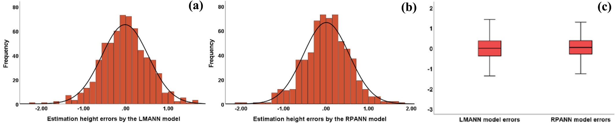
We examined the performances of the LM and RP algorithms in tree height prediction, with the disadvantages and restrictions of the standard back-propagation algorithm ([20], [55], [77]). The low dispersion of predicted values around the 1:1 line throughout the observed range of values (Fig. 5a, Fig. 5b) indicates that both ANN models had similar adjustments to the data used in model construction. Moreover, both ANN models showed better adaptation to the fitting data set than the fixed (Fig. 5c), mixed (Fig. 5d) and generalized (Fig. 5e) models. Furthermore, the statistical evaluation of the null hypothesis (H0: intercept = 0 and H0:slope = 1) for the linear relatonship hobs = intercept + slope · hpred was performed for all models (Fig. 5). The null hypotheses were not rejected at α=0.05 for either ANN models, indicating no significant differences between the 45 degree line and the linear trendline derived by the observed and the estimated height values (Fig. 5a, Fig. 5b). Finally, the RPANN model (Fig. 5b) appeared to provide slightly more accurate fitting to the observed data as compared to the LMANN model (Fig. 5a). The distribution of prediction errors from ANN models (Fig. 6a, Fig. 6b) revealed a frequency peak at zero and a rapid decline of the frequency at larger error values, thus corroborating that both ANN models are well-trained networks. Nonetheless, it is worth noting that the most accurate predictions were obtained by the best RPANN model, with a RMSE value of 2.25% lower than the error obtained from the best LMANN model.
Fig. 5 - Forty-five-degree plots with the linear trendline of height estimations obtained by (a) LMANN, (b) RPANN, (c) fixed, (d) mixed, and (e) generalized models.
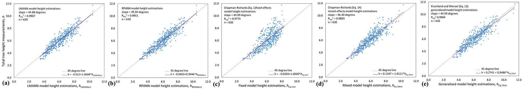
Fig. 6 - Errors histogram for height estimations obtained by the (a) LMANN, (b) RPANN models, and (c) errors box plots for both ANN models using the training data set.
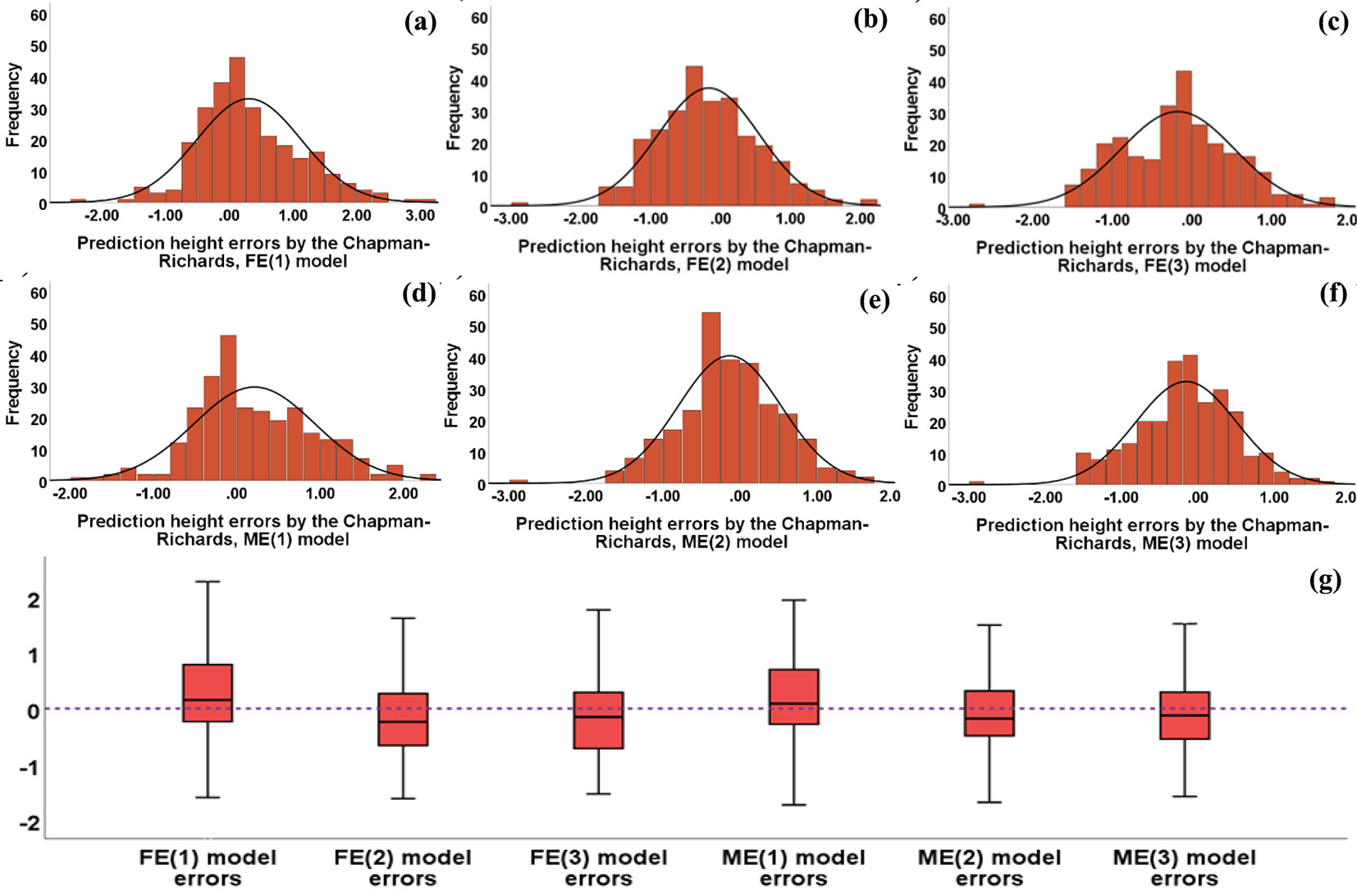
The prediction errors histograms and the relative errors box plots (Fig. 7, Fig. 8), along with the validation statistics presented in Tab. 4, clearly show that the RPANN model provided the most accurate and reliable prediction results as compared to the other models tested. The variability of the prediction errors (CV%) of the RPANN model was approximately 2.43%, which was lower than that of the LMANN model, and 1.47% lower than the variability derived from the Chapman-Richards mixed effect calibrated model [ME(3)]. The distribution analysis of prediction errors for all tested models suggested that the performances of the RPANN model are superior to those of all the other un-calibrated and calibrated models. Therefore, we conclude that the RPANN model provides the best performances in the estimation and prediction of tree height, as compared with fixed, generalized, fixed-calibrated and mixed calibrated models.
Fig. 7 - Errors histograms for height predictions obtained by (a) LMANN, (b) RPANN, (c) Chapman-Richards [eqn. 1 - FE(0)], (d) Krumland & Wensel (eqn. 13 - GM) models, and (e) errors’ box plots for all models using the validation data set..
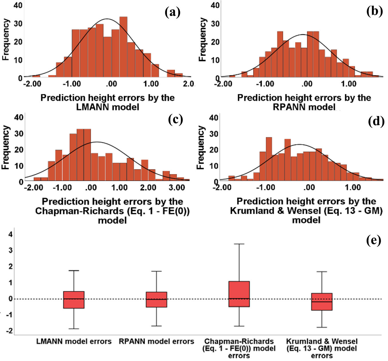
Fig. 8 - Errors histograms for height predictions obtained by the Chapman-Richards (a) FE(1), (b) FE(2), (c) FE(3), (d) ME(1), (e) ME(2), and (f) ME(3) models, and (g) errors box plots for all models using the validation data set.
Conclusions
In this study, equations for height prediction were developed for Cedrus libani plantations, which involved the evaluation of five alternative modeling methods: (i) the Generalized (GM); (ii) the non-calibrated fixed-effects [FE(0)]; (iii) the calibrated fixed-effect, using 1 to 3 calibration trees per plot [FE(1-3)]; (iv) the calibrated mixed-effects using 1 to 3 calibration trees per plot [ME (1-3)]; and (v) the ANNs using two different learning algorithms, the RP and the LM. As compared to the FE, all the constructed models (generalized, adjusted FE, ME, LMANN and BPANN) gave better performance, providing accurate and reliable tree height predictions. As expected, the predictive ability of the adjusted and ME models improved with increasing the calibration sample size. However, increasing the number of trees used for calibration had a minimal effect on the accuracy of the models.
The LMANN and RPANN models constructed in the present work showed reliable abilities to generalize from the input data and gave accurate predictions of the total tree height variable. Both alternatives exhibited similar performance in the construction phases, in addition to the ability to generalize. Based on the cumulative results from all approaches, the resilient propagation algorithm was more effective in predicting total stem height of C. libani growing in Turkey. The effectiveness and efficiency of ANN modeling in general and, specifically of the resilient propagation algorithm, along with the fit to the current dataset, the potential of this modeling approach to forest management, are clear. This direction is being followed in future research.
Author contribution
Y.K.: conceptualization, editing, results evaluation; M.D.: methodology, investigation, formal analysis, writing, review, editing; R.Ö.: methodology, investigation, formal analysis, review, writing, editing; Z.S.: data collection, data curation.
Acknowledgements
We thank the Turkish General Directorate of Forestry for its contribution to field work. We also thank Prof. Steve Woodward from University of Aberdeen for his valuable comments and suggestions for revising the English grammar of the text.
Funding
This work was financially supported by the Scientific Research Project Coordination Unit of the Suleyman Demirel University, Isparta, Turkey (project no. 2262-YL-10).
References
Gscholar
Gscholar
Gscholar
Gscholar
Gscholar
Gscholar
Gscholar
Gscholar
Gscholar
Gscholar
Authors’ Info
Authors’ Affiliation
Ramazan Özçelik 0000-0003-2132-2589
Faculty of Forestry, Isparta University of Applied Sciences, East Campus, 32260 Isparta (Turkey)
Faculty of Agriculture, Forestry and Natural Environment, School of Forestry and Natural Environment, Aristotle University of Thessaloniki, GR-54124 Thessaloniki (Greece)
Ministry of Agriculture and Forestry, VI Regional Directorate, 27002 Burdur (Turkey)
Corresponding author
Paper Info
Citation
Karatepe Y, Diamantopoulou MJ, Özçelik R, Sürücü Z (2022). Total tree height predictions via parametric and artificial neural network modeling approaches. iForest 15: 95-105. - doi: 10.3832/ifor3990-015
Academic Editor
Angelo Rita
Paper history
Received: Oct 04, 2021
Accepted: Jan 11, 2022
First online: Mar 21, 2022
Publication Date: Apr 30, 2022
Publication Time: 2.30 months
Copyright Information
© SISEF - The Italian Society of Silviculture and Forest Ecology 2022
Open Access
This article is distributed under the terms of the Creative Commons Attribution-Non Commercial 4.0 International (https://creativecommons.org/licenses/by-nc/4.0/), which permits unrestricted use, distribution, and reproduction in any medium, provided you give appropriate credit to the original author(s) and the source, provide a link to the Creative Commons license, and indicate if changes were made.

Web Metrics
Breakdown by View Type
Article Usage
Total Article Views: 35915
(from publication date up to now)
Breakdown by View Type
HTML Page Views: 29827
Abstract Page Views: 3252
PDF Downloads: 2215
Citation/Reference Downloads: 7
XML Downloads: 614
Web Metrics
Days since publication: 1547
Overall contacts: 35915
Avg. contacts per week: 162.51
Article Citations
Article citations are based on data periodically collected from the Clarivate Web of Science web site
(last update: Mar 2025)
Total number of cites (since 2022): 4
Average cites per year: 1.00
Publication Metrics
by Dimensions ©
Articles citing this article
List of the papers citing this article based on CrossRef Cited-by.
Related Contents
iForest Similar Articles
Research Articles
The use of tree crown variables in over-bark diameter and volume prediction models
vol. 7, pp. 132-139 (online: 13 January 2014)
Research Articles
Height-diameter models for maritime pine in Portugal: a comparison of basic, generalized and mixed-effects models
vol. 9, pp. 72-78 (online: 11 June 2015)
Research Articles
Exploring machine learning modeling approaches for biomass and carbon dioxide weight estimation in Lebanon cedar trees
vol. 17, pp. 19-28 (online: 12 February 2024)
Research Articles
Estimation of stand crown cover using a generalized crown diameter model: application for the analysis of Portuguese cork oak stands stocking evolution
vol. 9, pp. 437-444 (online: 02 December 2015)
Research Articles
Compatible taper-volume models of Quercus variabilis Blume forests in north China
vol. 10, pp. 567-575 (online: 08 May 2017)
Research Articles
Nonlinear mixed model approaches to estimating merchantable bole volume for Pinus occidentalis
vol. 5, pp. 247-254 (online: 24 October 2012)
Research Articles
Modeling stand mortality using Poisson mixture models with mixed-effects
vol. 8, pp. 333-338 (online: 05 September 2014)
Research Articles
Tree volume modeling for forest types in the Atlantic Forest: generic and specific models
vol. 13, pp. 417-425 (online: 16 September 2020)
Research Articles
Allometric models for estimating biomass, carbon and nutrient stock in the Sal zone of Bangladesh
vol. 12, pp. 69-75 (online: 24 January 2019)
Research Articles
Analyzing regression models and multi-layer artificial neural network models for estimating taper and tree volume in Crimean pine forests
vol. 17, pp. 36-44 (online: 28 February 2024)
iForest Database Search
Search By Author
Search By Keyword
Google Scholar Search
Citing Articles
Search By Author
Search By Keywords
PubMed Search
Search By Author
Search By Keyword


