Compatible taper-volume models of Quercus variabilis Blume forests in north China
iForest - Biogeosciences and Forestry, Volume 10, Issue 3, Pages 567-575 (2017)
doi: https://doi.org/10.3832/ifor2114-010
Published: May 08, 2017 - Copyright © 2017 SISEF
Research Articles
Abstract
Compatible taper and volume models were created for Quercus variabilis Blume (cork oak) forests in North China. 174 trees were felled to obtain stem analysis data. Linear mixed effects analyses were used in modelling. Firstly, a bark thickness model was built. Then diameter at breast height over bark (DBHob) for the inner layers of the 174 trees could be calculated, based on which a total volume model was built. The estimated volume and a specific parameter restriction were then substituted into a polynomial taper model, finally the taper model was fitted and compatible taper and volume models were obtained. Four sets of models based on different data sets were separately built and compared through coefficients of determination (R2), root mean square error (RMSE), value of Akaike’s information criterion (AIC), residuals plots and histograms of residuals. Models based on data of the analyzed stems without ramicorns and simultaneously with relative diameter under 1.5 were chosen as the most precise. Further testing of the chosen models using the jackknife method for the bark thickness and total volume models and a validation data set for the taper model verified that those models can be used to predict bark thickness, diameter at a specific point along the stem, merchantable volume and total stem volume of cork oak forests in North China within specific tree diameter at breast height and height ranges.
Keywords
Quercus variabilis Blume, Dummy Variable, Box-Cox Transformation, Linear Mixed Effects Models, Compatible Taper-Volume Model
Introduction
Compatible taper-volume models are flexible tools for estimating total and merchantable tree volume that can meet the demands of market trends as product specifications change. A compatible taper-volume estimation system contains a taper equation and a total volume equation. The taper equation can provide estimations of diameter at a given height up a tree and merchantable tree volume ([8]), and the total volume equation can easily estimate the total volume of a tree. Both models require diameter at breast height over bark (DBHob) and height as inputs. Compatible taper-volume estimation systems allow the volume computed by integration of the taper equation from the ground to the top of the tree to equal that calculated by a total volume equation.
Taper and volume estimation systems can be divided into two types: Type (1), the total volume model is directly derived through integration of the taper equation; Type (2), equation form of the total volume model is independent from the taper equation. For type (1), two methods can be used to estimate parameters of the two models: Method (1), firstly fit the taper equation, then the volume model with its parameters can be directly obtained by integration ([26]); Method (2), after obtaining the total volume equation through integration of the taper equation, the two models are fitted simultaneously to get their parameters by seemingly unrelated regression (SUR) or full information maximum likelihood (FIML) procedures ([18], [3], [36], [33]). For type (2), there are also two methods to estimate the parameters: Method (1), firstly estimate the total volume equation using the total volume observations, then substitute the estimated total volume from the volume model and a specific parameter restriction into a taper model, so that a compatible taper model can be estimated ([13], [25], [9], [28]); Method (2), simultaneous estimation of parameters of taper and volume models using SUR or FIML ([8]). Type (2) can provide an easily applied total volume model which can rapidly estimate tree volume ([8]), so this type is often preferred. Method (1) for Type (2) was especially useful when simultaneous estimation caused difficulty in achieving convergence, while Method (2) for Type (2) could make a reasonable compromise among the components in the system in the process of minimizing the sum of square errors ([10], [8]). Method (2) for Type (2) is more difficult when equations in the system have different numbers of observations. In this case, weights may be needed ([9], [8]). Some researchers compared the two methods and found that similar results were obtained ([10]). Method (1) for Type (2) also could make the system more flexible in application, i.e., for users who would like to use an existing volume table or volume equation to estimate volume; they can just use the taper model to obtain the diameter predictions ([9]).
A large number of compatible taper-volume systems based on type (1) have been created for oak species in Greece, America, Denmark, Spain and Mexico ([14], [45], [43], [36], [19]). Simple equations ([14], [45], [19]), variable exponent equations ([43]) or segmented-polynomial equations ([36]) were chosen for taper modelling. There has been no similar research for Quercus variabilis Blume, an important broadleaf tree species in North China, prior to the study reported here. The objective of our study was to develop a suitable compatible taper and volume estimation system including a polynomial taper equation and a total volume model basing on type (2) using Method (1), which can describe the stem profile well and provide accurate estimates of the stem volume of Quercus variabilis Blume (cork oak) forests in Northern China.
Material and methods
Measurements
174 trees from 104 plots with an area of 20 × 20 m for cork oak natural forests and plantations in North China were used in this study, 57 of those trees were from plantations (including 31 average trees and 26 dominant trees), and the other 117 trees were from natural forests (including 60 average trees and 57 dominant trees). These plots were created in the following locations with different site conditions and age distributions: Gao-Luo forestry station, Qi-Jiahe forestry station, Bei-Tan forestry station and Heng-He forestry station of Zhong-tiaoshan region in Shanxi province, collective forests of Da-Geliao village in Xingtai city of Hebei province, Si-Zuolou forestry station and Xi-Shan forestry station in Beijing. Measured and computed variables were as follows: (1) single tree variables including diameter at breast height over bark (DBHob), total tree height (H); (2) two perpendicular diameters inside-bark (dib) of every five rings of each disc, starting with the outermost ring, at 0.0, 0.5, 1.3 and 1.5 m above the ground and then every 1.0 m along the remainder of the stem which were measured and averaged. For the outermost layer of those stem analyzed trees, diameters outside-bark at those same heights were also measured; (3) log volumes were calculated using the Huber’s formula ([12]) where the top section was treated as a cone. Inside-bark total stem volumes (vib) were obtained by summing the log volumes and the volume of the top of the tree. Each tree contributed to the data set with as many height-diameter measurements from the stem analysis data as possible. Total stem volume (vib), diameter at breast height over bark (DBHob) and height (H) were repeated for each analyzed stem defined by 5 ring measurements ([30]). The data with DBHob equals to 0 (or H < 1.3 m) were deleted from the data set because the total volume under bark model (vib) would rely on DBHob as an independent variable. Finally, a total of 2358 bark thickness observations, 12814 diameter-height observations and 1299 volume observations from the 174 trees were obtained.
Model building
Four alternative modelling strategies were tried, because (1) a few analyzed stems (“trees”) had ramicorns and (2) some of the small analyzed stems had very high values of relative diameter (Rd, which is equal to dib/DBHib where dib is the diameter under bark at height h in cm, DBHib is the diameter at breast height under bark in cm, and h is the height from ground in m). Therefore, four sets of compatible bark thickness-taper-volume model systems were built, one for each dataset type: (i) System 1, using all the data of the analyzed stems; (ii) System 2, using data of analyzed stems without ramicorns; (iii) System 3, using data of analyzed stems with a Rd less than 1.5; (iv) System 4, using data of the analyzed stems without ramicorns and simultaneously with a Rd less than 1.5. Descriptive statistics for those data sets are shown in Tab. 1. Each model system included three models, i.e., a bark thickness model, a volume model and a taper model. Two dummy variables were used in System 1: Rddummy (Rddummy = 1 when Rd < 1.5, and 0 otherwise) and branch (branch = 1 when the tree has ramicorns, and branch = 0 otherwise). The dummy variable Rddummy was used in System 2, and dummy variable branch was used in System 3.
Tab. 1 - Summary statistics of four data sets used for modelling. (bt): bark thickness; (vib): stem total volume under bark; (dib): diameter under bark at height h; (h): height from ground; (H): total tree height; (DBHob): diameter at breast height over bark, breast height is 1.3 m height above the ground; (Rd): relative diameter, equal to dib/DBHib.
| Model type | Model system |
Sample number |
Range of age (year) |
Range of Rd |
Range of DBHob (cm) |
Range of H (m) |
Range of response variable |
|---|---|---|---|---|---|---|---|
| bt (cm) | 1, 3 | 2358 | 16-84 | 0.01-1.50 | 3.8-39.9 | 5.0-21.0 | 0.0-3.5 |
| 2, 4 | 2059 | 16-84 | 0.02-1.50 | 3.8-22.6 | 5.0-18.2 | 0.0-3.0 | |
| vib (m3) | 1 | 1299 | 5-84 | 1.00 | 0.3-39.9 | 1.4-21.0 | 0.00001-0.649 |
| 2 | 1201 | 5-84 | 1.00 | 0.3-23.1 | 1.4-18.2 | 0.00001-0.224 | |
| 3 | 1035 | 5-84 | 1.00 | 1.6-39.9 | 1.4-21.0 | 0.0002-0.649 | |
| 4 | 937 | 5-84 | 1.00 | 1.6-23.1 | 1.4-18.2 | 0.0002-0.224 | |
| dib (cm) | 1 | 12814 | 5-84 | 0.01-12.00 | 0.3-39.9 | 1.4-21.0 | 0.1-41.0 |
| 2 | 11336 | 5-84 | 0.01-12.00 | 0.3-23.1 | 1.4-18.2 | 0.1-25.5 | |
| 3 | 11419 | 5-84 | 0.01-1.50 | 1.6-39.9 | 1.4-21.0 | 0.1-41.0 | |
| 4 | 9942 | 5-84 | 0.01-1.50 | 1.6-23.1 | 1.4-18.2 | 0.1-25.5 |
For bark thickness models and volume models from the above-mentioned four systems, all data were used for model fitting. Before modelling, some explanatory and response variables (V) were transformed to new variables (tV) by Box-Cox transformation to make frequency distributions of those variables (tV) as close to normal distributions as possible. The following equation expresses a Box-Cox transformation ([40] - eqn. 1):
where V was the original response or explanation variable, tV was the response or explanatory variable after Box-Cox transformation, λ was the parameter in the Box-Cox transformation.
To establish bark thickness models and volume models, linear mixed effects analyses were used on transformed variables with the tree number (tree.no) as random effect. Model form was expressed as in eqn. 2 (see below - [35], [42]). The autocorrelation was addressed using three residual autocorrelation structures: a first-order autoregressive structure [AR(1)], a moving average structure [MA(1)] and combination of first-order autoregressive and moving average structures [ARMA(1.1)]. For bark thickness models of the four systems, tdibn, Rhn, natural, dominant, branch (for System 1 and System 3) and their interaction terms were chosen as possible explanatory variables and tbt is the response variable, where tdibn is equal to (tdib)n (n=1, 2, …, 5), tdib is the transformed diameter under bark at height h by the Box-Cox method (cm), Rhn is equal to (Rh)n (n=1, 2, …, 5), Rh is the relative height and equal to h/H, where h is height from ground (m), H is total tree height (m); natural and dominant are dummy variables to define the forest origin and the tree size, respectively: natural = 1 when the origin was a natural forest, natural = 0 in the case of plantations; dominant = 1 when the tree is dominant, dominant = 0 otherwise); tbt is the transformed bark thickness by the Box-Cox method (cm). The dummy variable Rddummy was not used in System 1 and System 2 because the data used for fitting the tbt model were all with a Rd<1.5 (Tab. 1). For volume models of the four systems, tDBHob, tH, td2h, natural, dominant, branch (for System 1 and System 3), Rddummy (for System 1 and System 2) and their interaction terms were chosen as possible explanatory variables, while tvib was the response variable, where tDBHob, tH, and tvib are transformed diameter at breast height over bark, transformed total tree height and transformed stem total volume under bark by the Box-Cox method, respectively (cm, m, m3), td2h is the transformed d2h by the Box-Cox method, d2h is equal to DBHob× DBHob×H; the other variables have the same specifications as in the bark thickness models. DBHob of inner layers of the 174 trees were calculated by eqn. 3 (see below), where bark thickness (bt) could be obtained from the bark thickness model. Model parameters were estimated by the ordinary least squares method (OLS - eqn. 2):
where Y is the vector of the response variable; X is the vector of fixed-effect regressors; Z is the vector of random-effect regressors; β is the vector of fixed-effect coefficients; μ is the vector of the random-effect coefficients; ε is the vector of errors. DBHob (diameter at breast height over bark, cm) was obtained as follows (eqn. 3):
where DBHib is the diameter at breast height under bark (cm), breast height is 1.3m height from ground, and bt is the bark thickness (cm).
For each model system, an overall merit-based method was used to select model explanatory variables. Regression equations for bark thickness models and volume models with different variable combinations were compared. Four sets of optimal base equations were obtained by examining the coefficients of determination (R2) and root mean square errors (RMSE); then the Akaike’s information criterion (AIC) was used to successively determine the best random-effects combination and the best residual autocorrelation structure for each optimal base model to obtain four sets of optimal tbt models and tvib models. For those optimal models, residual distribution homogeneity and model bias were visually checked by residual plots with loess regression lines overlaid on the plots. For an unbiased model, a loess line should be flat and located at the zero value on the vertical axis in the residual plot ([17]). Normality of residuals was checked with histograms of residuals and by using a Shapiro-Wilk test (probabilities of type I error or p-values < 0.05 indicate a departure from a normal distribution). Finally, bt models and vib models were obtained by back-transforming tbt models and tvib models (see eqn. 4, where exp is the natural exponential function, other notations have the same meanings with those in eqn. 1) and the residuals were also examined (eqn. 4):
For taper modelling of the four systems, a subset of data (80%) from the analyzed stems were randomly selected for the fitting phase, while the remaining data were used for model validation ([28], [3], [33]). Using the fitting data, the estimated total volume by the previously built total volume model (vib model) and a specific parameter restriction (see eqn. 7 below) could be substituted in a polynomial taper model (see eqn. 5 and eqn. 6 below - [13]), then the parameters of the taper models could be fitted by ordinary least squares (OLS - eqn. 5, eqn. 6, eqn. 7):
where dib is the diameter under bark at height h (cm), h is the height above the ground (m), H is the total tree height (m), Vv is the estimated stem total volume under bark from a total volume model (m3), ci terms are model parameters (i=1, 2, 3, …, 6).
To make taper modelling simpler, statistic Y can be calculated according to eqn. 8 (see below) and then the Y models were fitted firstly, i.e., the estimated values of total volume obtained by the vib model and a specific parameter restriction (see eqn. 7) were substituted into eqn. 8 instead of into eqn. 5. Linear mixed effects models (Y) with variables Zn (n=1, 2, ..., 6), dummy variable Rddummy (for System 1 and System 2) and dummy variable branch (for System 1 and System 3) as fixed factors and with tree number (tree.no) and dummy variable natural as random factors were fitted. Whether or not to include any particular estimated parameter was decided by the significance of a t-test. The autocorrelation was also addressed using the above-mentioned three residual autocorrelation structures. Then dib models can be obtained by eqn. 9 and the residuals were also examined (eqn. 8, eqn. 9):
Similarly, the R2, RMSE , AIC value, residual plots with loess regression lines overlaid on the plots and histograms of residuals of the Y models and dib models were tested. Then four sets of optimal regression equations (Y models and dib models) were selected.
To sum up, four sets of data (with a bark thickness model, a volume model and a taper model in each of them) were used for modelling and the most suitable set was then selected using the above-mentioned statistics and residual plots.
Optimal model system evaluation
After the selection of the optimal model system, representing essentially the best dataset, the transformed bark thickness model (tbt) and the transformed volume model (tvib) in it were tested by the leave-one-out Jackknife method ([39], [38]). The residual ranges and prediction ranges of the models and their corresponding jackknife tests were compared. Mean biases (Bias) and mean absolute biases (MAD) of the back-transformed vib model were also assessed for each diameter classes.
For the taper model in the optimal model system, the predictive performance of dib model was evaluated using the validation data set. The residual ranges and prediction ranges based on the validation data set were compared with those based on the fitting data set. Mean biases (Bias) and mean absolute biases (MAD) which were computed respectively using the fit data and validation data were assessed by position (percent relative height, i.e., 5%, 10%, 15%, …, 95%). Finally, the fitting and validation datasets were combined, the taper model (Y and dib) was refitted and the corresponding statistics and plots were examined again ([28]).
Results
Four sets of models
The p-value, R2 and RMSE of eight models (tbt, tvib, Y, bt vib and dib) in each model system are shown in Tab. 2. R2 values were higher than 0.85 for all the models and values of RMSE of all the models were low compared to the ranges of response variables (Tab. 1, Tab. 2). Probabilities of type I errors of all the models were lower than 0.05 (Tab. 2). Overall, models in System 4 had higher R2 and lower RMSE (Tab. 2). The loess curves of models in System 4 were closest to the x-axis, followed by those of System 2, then those of System 3, and models in System 1 with the biggest deviation from the x-axis; this means that models in System 4 had much lower bias than those in the other three systems. Therefore, System 4 was the optimal model system (only some of the residuals plots are shown in this paper, see below).
Tab. 2 - Values of fitting statistics for eight models in four modeling systems. (bt): bark thickness; (vib): stem total volume under bark; (dib): diameter under bark at height h; (tbt) and (tvib): transformed values of bt and vib by the Box-Cox method; (Y): calculated according to eqn. 8; (p-value): probability of type I error in Shapiro Wilks test (for the tbt and tvib models) and probability of type I error in Kolmogorov-Smirnov test (for the Y models); (R2): coefficient of determination; (RMSE): root mean square errors.
| Models type |
Model system |
Transformed models tbt (cm), tvib (m3) or Y |
Back-transformed models bt (cm), vib (m3) or dib (cm) |
|||
|---|---|---|---|---|---|---|
| p-value | R 2 | RMSE | R 2 | RMSE | ||
| bt (cm) | 1, 3 | < 2.2e-16 | 0.90 | 0.22 | 0.86 | 0.24 |
| 2, 4 | 9.646e-13 | 0.94 | 0.15 | 0.92 | 0.15 | |
| vib (m3) | 1 | 3.343e-12 | 0.99 | 0.061 | 0.99 | 0.006 |
| 2 | 9.195e-08 | 0.99 | 0.043 | 0.99 | 0.003 | |
| 3 | 6.921e-09 | 0.99 | 0.066 | 0.99 | 0.006 | |
| 4 | 2.14e-06 | 0.99 | 0.044 | 0.99 | 0.003 | |
| dib (cm) | 1 | < 2.2e-16 | 0.91 | 0.32 | 0.97 | 0.84 |
| 2 | < 2.2e-16 | 0.91 | 0.32 | 0.97 | 0.67 | |
| 3 | < 2.2e-16 | 0.95 | 0.21 | 0.97 | 0.80 | |
| 4 | < 2.2e-16 | 0.96 | 0.20 | 0.98 | 0.61 | |
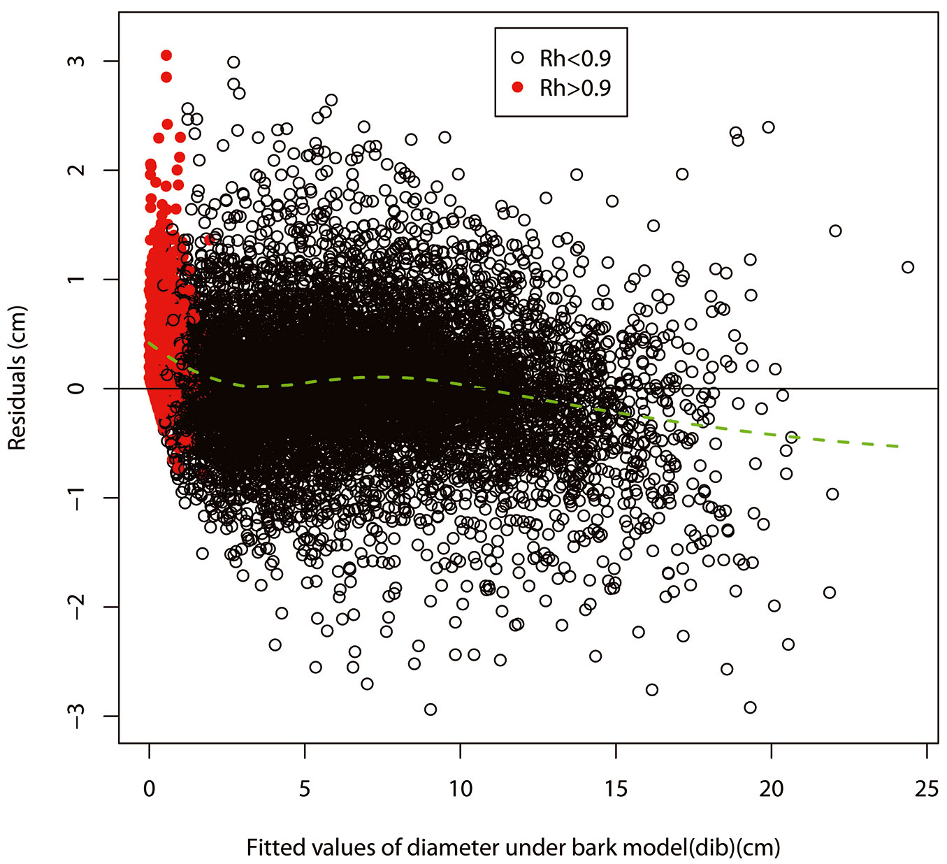
Equation forms, coefficients and standard errors of coefficients of the models in System 4 are shown in Tab. 3, Tab. 4 and Tab. 5. All the coefficients were significant at α=0.001 confidence level and standard errors of coefficients were small compared to the coefficients (Tab. 3, Tab. 4 and Tab. 5). A first-order autoregressive structure [AR(1)], a moving average structure [MA(1)] and a combination of first-order autoregressive and moving average structures [ARMA(1.1)] were respectively elected as the best to address the autocorrelation of the tbt model, tvib model and Y model, respectively (Tab. 3, Tab. 4 and Tab. 5). Predicted value ranges and residual ranges of those models are also shown in Tab. 3, Tab. 4 and Tab. 5. Residual plots of the bark thickness model (bt), volume model (vib) and taper model (dib) in System 4 fitted to the combined datasets are shown in Fig. 1, Fig. 2 and Fig. 3, respectively. In general, the loess lines are represented by flat lines located at the baselines, except for the trees with a relative height (Rh) higher than 0.9 for the residual plot of the taper model. Heteroscedasticity was not obvious in the transformed bark thickness model (tbt), transformed volume model (tvib) and the taper models (Y and dib), while a weak heteroscedasticity could be detected in the back-transformed thickness model (bt) and in the back-transformed volume model (vib). Low p-values of the Shapiro Wilks tests or Kolmogorov-Smirnov tests (Tab. 2) and histograms of residuals (data not shown) suggested that residuals of the models in System 4 did not have a normal distribution. Skewness was not detected in these distributions, but kurtosis was.
Tab. 3 - Summaries for the tbt and bt models in System 4. The type III sum of squares was used in those models. (bt): bark thickness (cm); (tbt) and (tdib): transformed values of bt and dib by the Box-Cox method, i.e., tbt=(bt0.538-1)/ 0.538, tdib=(dib0.716-1)/0.716; (dib): diameter under bark at height h (cm); (Rh): relative height and equal to h/H; (h): height from ground (m); (H): total tree height (m); (natural): dummy variable (natural = 1 for natural forests; natural = 0 for plantations); (ai): model parameters (i=1, 2, 3, ..., n); (SE): standard errors of coefficients; (ρ): the parameter for first-order autoregressive structure [AR(1)]; (σ2): the residual variance; (σai2): the variance for the random effects. (***): p<0.001.
| Model | Equation form | Coefficients (± SE) | Predicted value range/ Residual range |
||
|---|---|---|---|---|---|
| Model (Entire data) |
Jackknife | ||||
| tbt | tbt = a0 + a1 · tdib5/104 + a2 · dib4/103 + a3 · tdib3/102 + a4 · tdib + a5 · Rh + a6 · Rh2 + a7 · Rh3 + a8 · Rh4 + a9 · natural |
a 0 | -0.881 ± 0.058*** | (-1.58, 1.22)/ (-0.61, 0.56) |
(-1.60, 1.24)/ (-0.64, 0.60) |
| a 1 | -0.277 ± 0.071*** | ||||
| a 2 | 0.669 ± 0.160*** | ||||
| a 3 | -0.495 ± 0.101*** | ||||
| a 4 | 0.278 ± 0.018*** | ||||
| a 5 | -3.182 ± 0.201*** | ||||
| a 6 | 8.094 ± 0.882*** | ||||
| a 7 | -8.695 ± 1.426*** | ||||
| a 8 | 3.327 ± 0.745*** | ||||
| a 9 | 0.089 ± 0.022*** | ||||
| ρ | 0.403 | ||||
| σ2 | 0.025 | ||||
| σa02 | 0.013 | ||||
| bt | bt = (0.538 · tbt + 1)(1⁄0.538) | - | - | (0.03, 2.56)/ (-0.60, 0.74) |
- |
Tab. 4 - Summaries for the tvib and vib models in System 4. The type III sum of squares was used in those models; (tvib), (tH) and (td2h): transformed values of vib, H and d2h by the Box-Cox method, i.e., tvib=(vib0.18-1)/0.18, tH=(H0.81-1)/0.81, td2h=[(d2h)0.21 -1]/0.21; (d2h): equal to DBHob·DBHob·H; (DBHob): diameter at breast height over bark (cm); (H): total tree height (m); (vib): stem total volume under bark (m3); (bi): model parameters (i=1, 2, 3, ..., n); (SE): standard errors of coefficients; (θ): the parameter for moving average structure [MA(1)]; (σ2): the residual variance; (σbi2): the variance for the random effects. (***): p<0.001.
| Model | Equation form | Coefficients (± SE) | Predicted value range/ Residual range |
||
|---|---|---|---|---|---|
| Model | Jackknife | ||||
| tvib | tvib = b0 + b1·td2h + b2·tH | b 0 | -4.488 ± 0.007*** | (-4.296,-1.244)/ (-0.218, 0.180) |
(-4.290,-1.233)/ (-0.243.0.216) |
| b 1 | 0.125 ± 0.002*** | ||||
| b 2 | -0.021 ± 0.005*** | ||||
| θ | 0.467 | ||||
| σ2 | 0.002 | ||||
| σb02 | 0.002 | ||||
| vib | vib = (0.18·tvib+1)(1⁄0.18) | - | - | (0.0003.0.245)/ (-0.020, 0.018) |
- |
Tab. 5 - Summaries for Y and dib models in System 4. The type III sum of squares was used in those models. (dib): diameter under bark at height h (cm); (h): height from ground (m); (H): total tree height (m); (Y): calculated according to eqn. 8; (Zn) (n =1, 2, ..., 6): calculated according to eqn. 6; (Vv): estimated stem total volume under bark from stem total volume model (m3); (ci): model parameters (i=1, 2, 3, ..., n); (SE): standard errors of coefficients; (ρ): the parameter for first-order autoregressive structure [AR(1)]; (θ): the parameter for moving average structure [MA(1)]; (σ2): residual variance; (σci2): variance for the random effects (including natural and tree.no.). (***): p<0.001.
| Model | Equation form | Coefficients (± SE) | Predicted value range / Residual range | |||
|---|---|---|---|---|---|---|
| Entire data | Fit data | Validation data | ||||
| Y | Y = c3·Z3 + c4·Z4 + c5·Z5 + c6·Z6 + [8·(1-(c3⁄4)-(c4⁄5)-(c5⁄6)-(c6⁄7))]·Z7 |
c 3 | 33.972 ± 1.545*** | (0.00, 4.04)/ (-1.18, 1.48) |
(0.00, 4.05)/ (-1.19, 1.24) |
(0.00, 3.12)/ (-1.81, 1.45) |
| c 4 | -125.749 ± 8.907*** | |||||
| c 5 | 229.692 ± 18.913*** | |||||
| c 6 | -211.380 ± 17.418*** | |||||
| ρ | 0.738 | |||||
| θ | -0.359 | |||||
| σ2 | 0.043 | |||||
| σc32 | 0.050; 8.117 | |||||
| σc42 | 0.210; 24.145 | |||||
| dib | dib = [(40000·Vv·Y)/(π·H)](1/2) | - | - | (0.00, 24.39)/ (-2.94, 3.03) |
(0.00, 24.40)/ (-2.91, 2.70) |
(0.00, 22.94)/ (-2.60, 3.05) |
Fig. 1 - Loess residual plot of the back-transformed bark thickness model in System 4. The solid horizontal line indicates the baseline, while the red dotted line represents the loess curve.
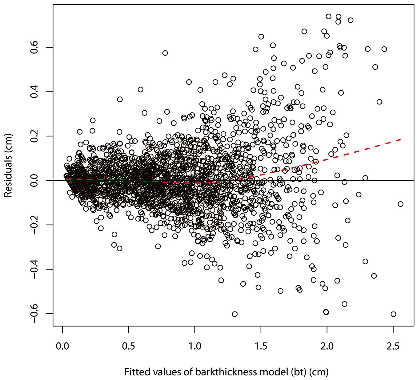
Fig. 2 - Loess residual plot of the back-transformed total stem volume inside bark model in System 4. The solid horizontal line indicates the baseline, while the red dotted line represents the loess curve.
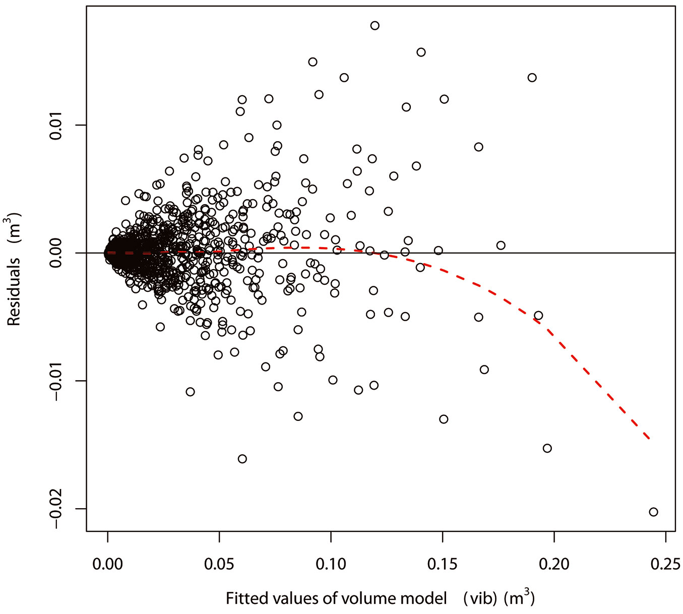
Fig. 3 - Loess residual plot of the back-transformed diameter inside bark model in System 4. The red closed circles represent the residuals under the condition of relative height > 0.9 and the black open circles represent the residuals under the condition of relative height <0.9. The solid horizontal line indicates baseline and the green dotted line indicates loess curve.
Evaluation of the models in System 4
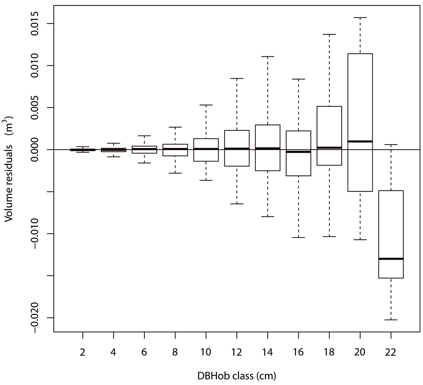
Predicted value ranges and residual ranges from the Jackknife validations for the transformed bark thickness model (tbt) and the transformed volume model (tvib) in System 4 were similar with those obtained from fittings and are shown in Tab. 3 and Tab. 4. Scatter distribution in residual plots from fittings and that from the jackknife validations were similar, as well as the frequency distributions in histograms of residuals (data not shown). Moreover, frequencies, mean bias (Bias) and mean absolute deviation (MAD) of the back-transformed volume model (vib) were tested and the corresponding results are listed in Tab. S7 (Supplementary material). The overall values of Bias and MAD were 0.09·10-3 m3 and 1.76·10-3 m3 (Tab. S7 in Supplementary material). Both Bias and MAD in different DBHob classes had an increasing trend with increasing DBHob. However, all the values of Bias and MAD were very small compared to the magnitudes of predicted values (see Tab. S4 and Tab. S7 in Supplementary material), so the vib model could provide accurate prediction within the DBHob range of 1.6 to 23.1 cm and within the H range of 1.4 to 18.2 m. The box plot of residuals in each diameter class for the vib model is shown in Fig. 4.
Fig. 4 - Box plot of residuals versus diameter at breast height over bark class for the volume inside bark model in System 4.
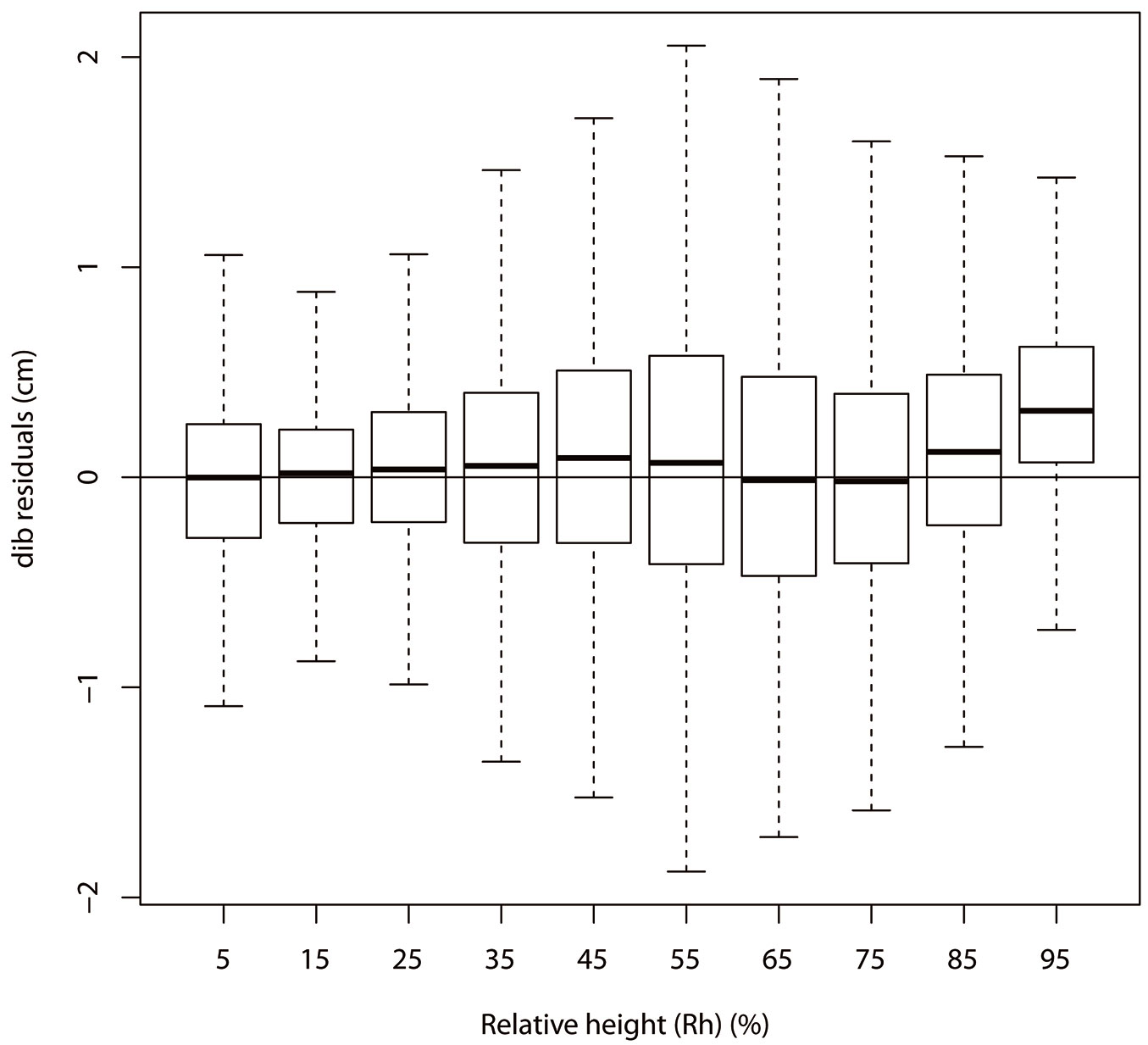
Residual plots, predicted value ranges, residual ranges, Bias and MAD of the taper model fitted with the entire data set and the fitting data set were very close to each other, while the corresponding statistics of the taper model fitted with the validation data set were a little different (Tab. S5 and Tab. S8 - Supplementary material). All the values of the Bias and MAD were small compared to the magnitude of predicted values (see Tab. S5 and Tab. S8 in Supplementary material). For the dib model built using the entire data, the overall values of Bias and MAD were 0.06 cm and 0.45 cm, and the Bias and MAD in different relative height classes (Rhg) respectively ranged from -0.04 to 0.40 cm and from 0.29 to 0.60 cm (Tab. S8 in Supplementary material). This dib model could provide accurate predictions within a DBHob range of 1.6 to 23.1 cm and within an H range of 1.4 to 18.2 m. Fig. 5 shows a box plot of residuals versus relative height (Rh) for the dib model.
Fig. 5 - Box plot of residuals versus relative height for the taper model in System 4.
Discussion
Equation form of total volume model
Various forms of volume models have been reported in the literature, such as the model represented by eqn. 10 (see below) proposed by Schumacher & Hall in 1933 ([1], [9]), eqn. 11 ([25]), eqn. 12 ([8]), eq. 13 ([16]) and eqn. 14 ([28]). These equations are shown below (eqn. 10 to eqn. 14):
where V is the volume, DBH is the diameter at breast height, H is the total height, ai terms are model parameters, e is the base of the natural logarithm. Some of the volume models have a conceptual basis in the geometry of solids of revolution and have a constant form factor ([1]). In fact, the form of a tree depends upon the actual tree size, e.g., there was a downward trend of form factor along with increased tree height in our study. Some volume models in some studies explicitly represented change of a form factor, which was defined as a function of diameter at breast height, total height, stem height at a predetermined fraction of diameter at breast height outside bark, or the ratio of this height to total height ([1], [37]). However, there is always a problem of heterogeneity in those nonlinear volume models. For removing heterogeneity of variance, weighted non-linear regression was usually used to estimate parameters ([28]). However, computing a suitable weighting variable was awkward. Another simple and common way of removing heterogeneity of residual variance is performing a transformation to stabilize variance. In our study, the Box-Cox transformation was used, then the linear mixed effect equation of the transformed volume was built and no heterogeneity was detected. Meanwhile, bias of the back-transformed volume model was found to be small, and so no correction factor was used in this study. Additionally, an overall merit-based method was used to select model explanatory variables for the volume model, so the volume model did not have a conceptual basis in the geometry of solids of revolution and did not explicitly represent change of a form factor.
In the application of a mixed effect model, when a sub-sample of the dataset is available to calculate the random effects, users can calibrate the coefficients of the linear mixed effect model (“lme” - [44]) and then obtain unbiased predictions. However, predicting the random effects is hard for users. Actually, in our study the bias was found small enough, even though just the fixed effect was considered in prediction; thus, there was no need to calibrate the random effect before using the “lme” volume model. Population predictions of volume for a new tree can be obtained using fixed effect coefficients.
Similar features can be found in the bark thickness model, which was also a linear mixed effect equation using variables transformed by the Box-Cox method.
The simple taper model
According to several studies in the literature ([8], [32], [15]), taper equations can be grouped in three types: (1) simple taper equations ([4], [22], [6], [7], [31], [13], [9], [41]); (2) segmented taper equations ([27], [5], [34], [10], [18]); (3) variable exponent taper equations ([20], [29], [2], [23], [21]). Some researchers have pointed out that segmented taper equations and variable exponent taper equations can sometimes provide more flexible descriptions of tree profiles than simple taper equations; variable exponent taper equations usually have the least bias and best predictive abilities among the three kinds of models ([20], [29], [28], [32]). For simpler equations, the presence of larger residuals located in the lower bole (the stump region) is pronounced in some studies ([15]). However, a shortcoming of variable exponent taper equations is that they cannot be analytically integrated to calculate total stem or log volumes ([8], [33]). Additionally, segmented taper equations and variable exponent taper equations suffer from statistical complexity, difficulties in parameter estimation and difficulties of being understood and correctly used by forest managers. Therefore, when simplicity of use is an objective, the simple taper model would be a good choice, despite its lower accuracy in the lower bole ([26]).
A polynomial taper equation ([13]) was used in this study. Larger residuals were only found at about 90% of stem height (Fig. 3, Fig. 5). The poorer performance observed in predictions at the stem top is negligible from a practical point of view ([11], [15]), as the top part of cork oak is usually collected for bio-fuel. As we are interested only in the middle part of the bole, a simple taper model can be used for practical purposes ([32]).
Ramicorns and relative diameter
Branches are an important aspect of tree form because they affect stem utilization. A ramicorn branch is a steep-angled branch diverging less than 30° from the main stem and significantly smaller than the main stem ([46]). In this study, the number of trees with ramicorns was very small. Additionally, the values of relative diameter for most of the computed trees in the data set were under 1.5, which is consistent with those in other studies ([5], [1], [8], [32], [24], [33], [15]). A few small trees estimated from inner rings had very high values of relative diameter (up to 12.0). These were very tiny “trees”, with ages of 5 years and a diameter at breast height under 1.0 cm.
We built four sets of compatible taper-volume model systems using all the data (Model system 1), using data of stems without ramicorns (Model system 2), data of stems with a Rd less than 1.5 (Model system 3) and data of stems without ramicorns and simultaneously with a Rd less than 1.5 (Model system 4). Performances of models using those four datasets were compared though the R2, RMSE, residual plots and histograms of residuals. It turned out that models in System 4 had the best performances, followed by System 2 and System 3, while models in System 1 had the worst performances (Tab. 2). Although a dummy variable (branch) to define ramnicorn trees was introduced in System 1 and System 3, performances of those models were still not good enough, partly because of the small number of sample trees with ramicorns. More data of trees with ramicorns need to be collected in order to get more integrated and accurate models. Performances of models in System 2 were much better than those of System 1 and System 3, and just a little poorer than those of System 4. However, System 2 contained the data of stems with a Rd bigger than 1.5, which were not common in practical application. Therefore, models in System 4 were selected as the most appropriate in terms of precision, lack of bias and practical application. They can be used to predict bark thickness, diameter at a specific point along the stem, merchantable volume and total stem volume of cork oak forests in North China within the specific ranges of DBH (1.6-23.1 cm) or H (1.4-18.2 m).
In System 4, data from four big trees were removed because they had ramicorns. Due to the small sample size for big trees, more big trees should be measured in the future to obtain a compatible taper-volume model system with a larger useable diameter span. It should be noted that if models created using System 4 are used for predictions of stems with ramicorn branches, then errors would be likely greater than those reported here. Therefore, we suggest that models created with System 4 can be used for predictions of stems without ramicorn branches and simultaneously with a relative diameter less than 1.5.
Conclusion
Linear mixed effect equations with tree number as random factor were used for bark thickness and volume modelling using variables transformed by the Box-Cox method to minimise heteroscedasticity. Using the polynomial equation reported by Goulding & Murray ([13]), linear mixed effect equations with tree number and natural (a dummy variable specifying the stand origin) as random factors were fitted during taper modelling.
Four sets of compatible taper-volume models systems using different data sets were established and compared. The models in System 4 had superior coefficients of determination (R2), root mean square errors (RMSE) and lack of bias than models from the other three systems and thus were selected as the most suitable in this study. Furthermore, the models in System 4 had good performances in jackknife validation or independent data set validation. Heteroscedasticity was not obvious in the transformed bark thickness model, transformed volume model and the taper model, while a weak heteroscedasticity could be detected in the back-transformed bark thickness model and back-transformed volume model. Residuals of the models in System 4 did not follow normal distribution. Skewness was not detected in these distributions, but they were slightly kurtotic.
Within the specified ranges of DBH (1.6-23.1 cm) or H (1.4-18.2 m) tested in this study, the compatible taper-volume models system can be used for predicting diameter at a specific point along the stem, merchantable volume and total stem volume of cork oak forests in North China.
Acknowledgements
This research was jointly supported by scientific and research base construction projects of Beijing Municipal Education Commission (SYSBL2009), forestry science promotion project of the State Forestry Bureau (2011-44), open fund project of Beijing Forestry University “985” advantage subject innovation platform (000-1108003), special fund project for forestry public service industry and research (201004021) and China Scholarship Council. We acknowledge the strong support from Zhong Tiaoshan National Forest Authority, Xingtai County Forestry Bureau, Si Zuolou forestry station and Xi Shan forestry station in Beijing.
Conghui Zheng and Yuzhong Wang have equally contributed to this work and should be regarded as co-first authors.
References
Gscholar
Authors’ Info
Authors’ Affiliation
Yuzhong Wang
Hebei Engineering and Technology Center of Forest Improved Variety, Hebei Academy of Forestry, Shijiazhuang 050000 (China)
Liming Jia
Songpo We
Caowen Sun
Jie Duan
Ministry of Education Key Laboratory of Silviculture and Conservation, Beijing Forestry University, Beijing 100083 (China)
School of Forestry, University of Canterbury, Christchurch 8140 (New Zealand)
Corresponding author
Paper Info
Citation
Zheng C, Wang Y, Jia L, Mason EG, We S, Sun C, Duan J (2017). Compatible taper-volume models of Quercus variabilis Blume forests in north China. iForest 10: 567-575. - doi: 10.3832/ifor2114-010
Academic Editor
Rupert Seidl
Paper history
Received: May 16, 2016
Accepted: Feb 22, 2017
First online: May 08, 2017
Publication Date: Jun 30, 2017
Publication Time: 2.50 months
Copyright Information
© SISEF - The Italian Society of Silviculture and Forest Ecology 2017
Open Access
This article is distributed under the terms of the Creative Commons Attribution-Non Commercial 4.0 International (https://creativecommons.org/licenses/by-nc/4.0/), which permits unrestricted use, distribution, and reproduction in any medium, provided you give appropriate credit to the original author(s) and the source, provide a link to the Creative Commons license, and indicate if changes were made.

Web Metrics
Breakdown by View Type
Article Usage
Total Article Views: 51638
(from publication date up to now)
Breakdown by View Type
HTML Page Views: 42318
Abstract Page Views: 3752
PDF Downloads: 4107
Citation/Reference Downloads: 38
XML Downloads: 1423
Web Metrics
Days since publication: 3344
Overall contacts: 51638
Avg. contacts per week: 108.09
Article Citations
Article citations are based on data periodically collected from the Clarivate Web of Science web site
(last update: Mar 2025)
Total number of cites (since 2017): 7
Average cites per year: 0.78
Publication Metrics
by Dimensions ©
Articles citing this article
List of the papers citing this article based on CrossRef Cited-by.
Related Contents
iForest Similar Articles
Research Articles
Nonlinear mixed model approaches to estimating merchantable bole volume for Pinus occidentalis
vol. 5, pp. 247-254 (online: 24 October 2012)
Research Articles
Modeling compatible taper and stem volume of pure Scots pine stands in Northeastern Turkey
vol. 16, pp. 38-46 (online: 22 January 2023)
Research Articles
Analyzing regression models and multi-layer artificial neural network models for estimating taper and tree volume in Crimean pine forests
vol. 17, pp. 36-44 (online: 28 February 2024)
Research Articles
Modelling taper and stem volume considering stand density in Eucalyptus grandis and Eucalyptus dunnii
vol. 14, pp. 127-136 (online: 16 March 2021)
Research Articles
Comparative analysis of taper models for Pinus nigra Arn. using terrestrial laser scanner acquired data
vol. 17, pp. 203-212 (online: 22 July 2024)
Research Articles
The use of tree crown variables in over-bark diameter and volume prediction models
vol. 7, pp. 132-139 (online: 13 January 2014)
Research Articles
Tree volume modeling for forest types in the Atlantic Forest: generic and specific models
vol. 13, pp. 417-425 (online: 16 September 2020)
Research Articles
Height-diameter models for maritime pine in Portugal: a comparison of basic, generalized and mixed-effects models
vol. 9, pp. 72-78 (online: 11 June 2015)
Research Articles
Estimation of stand crown cover using a generalized crown diameter model: application for the analysis of Portuguese cork oak stands stocking evolution
vol. 9, pp. 437-444 (online: 02 December 2015)
Technical Reports
Effects of different mechanical treatments on Quercus variabilis, Q. wutaishanica and Q. robur acorn germination
vol. 8, pp. 728-734 (online: 05 May 2015)
iForest Database Search
Search By Author
Search By Keyword
Google Scholar Search
Citing Articles
Search By Author
Search By Keywords
PubMed Search
Search By Author
Search By Keyword


