
Nonlinear mixed model approaches to estimating merchantable bole volume for Pinus occidentalis
iForest - Biogeosciences and Forestry, Volume 5, Issue 5, Pages 247-254 (2012)
doi: https://doi.org/10.3832/ifor0630-005
Published: Oct 24, 2012 - Copyright © 2012 SISEF
Research Articles
Abstract
The ability to predict cumulative bole volume to any predefined upper stem diameter on a standing tree is essential for estimating current inventory levels and making informed decisions regarding the management of forest resources. Several types of mathematical models have been developed to predict cumulative bole volume, requiring only the collection of low cost data but high accuracy tree measurements. This paper reports on the comparison of a variable-exponent taper model and a volume-ratio model for estimating inside-bark cumulative bole volume to three predefined upper stem diameters using stem analysis data Pinus occidentalis trees in La Sierra, Dominican Republic. Each sampled tree was measured at multiple points on the bole, making observations spatially correlated within the tree. Inference problems due to autocorrelation were addressed by using a nonlinear mixed-effects model fitted by restricted maximum likelihood (REML) and including two random parameter coefficients at tree level in each of the two models tested. Using an independent validation data set, the variable-exponent taper model with two random parameters demonstrated better predictive ability as compared to the volume-ratio model when estimating cumulative bole volume to the three predefined upper stem diameters. The taper model allows flexible volume estimation for the population average as well for specific trees.
Keywords
Nonlinear Mixed-effects Models, Restricted Maximum Likelihood, Taper Model, Volume-ratio Model, Random Coefficients, Calibration, Pinus occidentalis
Introduction
Regression analysis was initiated into forestry research more than 70 years ago. One common use of applying ordinary least squares and non-linear least squares techniques was to fit a regression model to predict volume content in the stem of a standing tree ([14]). The set of explanatory variables included in a volume model is relatively small and comprises tree dimensions that can be easily and accurately measured in the forest, i.e. stem diameter at breast height (D) and total tree or merchantable height (H).
Due to changes in utilization standards within the forest industry, many different bole-volume equations have been developed. Volume prediction to any merchantability limit has been accomplished in many ways, including: (1) a constrained volume equation for different merchantable limits that differed by a fixed amount ([2]); (2) expressing the merchantable volume for a given set of merchantability limits as a proportion of total tree volume, often called the “volume ratio approach” ([1]); and (3) stem profile equations which predict upper stem diameters at any point along the tree bole developed by Kozak ([19]). They can be integrated to give volume content within any portion of the tree bole. The first approach requires a cumbersome procedure. The last two approaches are more common.
Construction of taper and volume-ratio equations entails the compilation of longitudinal data on each tree, resulting in a lack of independence between observations and biased estimates of parameters if ordinary least squared techniques are used in constructing the models ([8]). Observations from the same unit of analysis, the trees, are correlated ([14], [11], [20]).
The fixed effects model that includes explanatory variables accounts for a part of the total variation in tree volume content. There is a residual variability component, representing differences in attributes acting at stand or tree level, that are difficult to observe, encompassing heredity and environmental factors, or even measurement errors, introducing a stochastic level of variability in tree volume content. Calama & Montero ([8]) stated: “The use of mixed models allows us to identify the different sources of stochastic variability that are not explained by the fixed part of the model by dividing the residual variance into different components”.
To properly analyze this type of data, the error structure inherent within the data must be considered in the modeling process. Even though ordinary least squares analysis provides unbiased parameter estimates in the presence of autocorrelation, it does not provide minimum variance estimators ([13]). The violation of the assumption of independence required by the linear regression model would make inferences and test of significance invalid ([30]). The properties of the least square estimators would be affected when observations are not independent, although the approach itself does not make assumption of independent observations.
In addition to being correlated, the data for the construction of taper and volume-ratio models is unbalanced. Each sample tree is measured by short sections and the desired volume (total or merchantable) is determined by summing up the volumes of all the sections in a tree. Often, the number of observations of cumulative bole volume will vary among trees, as short trees tend to have fewer sections than larger trees. The observed sample will be unbalanced by having unequal numbers of observations per subject ([13]).
Two general methods have been proposed to fit continuous, unbalanced, multilevel longitudinal data. The first proposed by Gregoire & Schabenberger ([14]) incorporates random subject effects, while the second models the correlation structure directly ([22]). The former employs nonlinear mixed effects models, inducing the correlations in the marginal distribution of observations from the same tree by random effects that vary across trees, to reduce the impact of autocorrelation. The second approach introduces an assumed correlation structure into a generalized least squares solution ([27]).
Mixed-effects models, consisting of both fixed and random-effects parameters have the advantage to allow for modeling of the variance-covariance matrix of correlated data ([31]). Using random effects to capture tree-to-tree variability allows for modeling the volume of the individual tree stem (subject specific) as well as the volume of the average tree (population specific - [26]). Jones ([17]) pointed out that modeling the variance-covariance structure directly or through random parameters indirectly was often equally effective in accounting for the within-subject correlation.
Pinus occidentalis Sw. is an endemic pine species of Hispaniola Island (Caribbean Sea). In Dominican Republic (DR), it is the single most abundant species with the ability to successfully grow and protect the acidic, shallow and infertile sandy soils which characterized the steeped slopes of the mountain ranges ([4]). In 1995, the species occupied approximately 302 500 hectares in the DR ([10]), representing more than the 95% of the species’ world-wide distribution. In terms of timber production, P. occidentalis is the most important in the DR, comprising approximately 95% of all timber harvested ([3]). The most valuable wood product from P. occidentalis stands is its timber, which is used for construction and furniture manufacturing. Other important wood products derived besides saw timber logs are poles and bars used in the tobacco industry.
Despite its economic and ecologic importance, this species has never been the subject of serious growth and yield studies, making it difficult to estimate current inventory levels and to account for the amount of volume harvested ([5]). Few volume equations are available for the species at a regional level ([23]). Existing equations have been developed to estimate single tree volume from breast height diameter and total height, but they do not enable product classification and did not consider the inherent difficulties derived from high correlation among observations taken on sample trees, since the parameter estimation method employed was solely based on ordinary least squares.
The primary objectives of this study were to: (1) fit both a variable-exponent taper equation and a total volume-ratio model to P. occidentalis data from La Sierra (Dominican Republic) using a mixed-effects modeling approach; (2) compare the accuracy and precision of each model based on evaluation criteria using an independent validation data set; and (3) recommend that best model for estimating merchantable volume for different utilization standards for this species. Parameter estimates along with their respective significance levels and goodness- of-fit statistics of the models tested will be reported.
Material and methods
Data set
The study area is a region of approximately 1800 km2 in the north central portion of Cordillera Central, Dominican Republic. Five natural stands of P. occidentalis were selected from three different ecological zones: two in subtropical dry forest; two from the subtropical very humid forest; and one in the subtropical humid forest.
To validate the models, the original data set was randomly divided into two parts. Eighty percent of the observations (n = 149) were used to develop the taper and volume-ratio models, and 20% (n = 39) to validate them. Summary statistics for both fitting and validation data sets for tree diameter at breast height, total tree height, and various merchantable volume measurements are listed in Tab. 1.
Tab. 1 - Descriptive statistics for the estimation and verification data sets of P. occidentalis trees.
| Datasets | Variables | Mean | St. Dev. | Min | Max |
|---|---|---|---|---|---|
| Estimation (n=149) |
Diameter at breast height (cm) | 29.8 | 8.31 | 11.5 | 53.5 |
| Total height (m) | 21.9 | 5.51 | 8.6 | 35 | |
| Total volume (m3) | 0.6 | 0.45 | 0.03 | 2.49 | |
| Cumulative volume (m3) to 4 cm top diameter | 0.59 | 0.45 | 0.03 | 2.49 | |
| Cumulative volume (m3) to 8 cm top diameter | 0.58 | 0.45 | 0.01 | 2.48 | |
| Cumulative volume (m3) to 14 cm top diameter | 0.54 | 0.46 | 0 | 2.46 | |
| Verification (n=39) |
Diameter at breast height (cm) | 30.32 | 9.13 | 9.2 | 53.1 |
| Total height (m) | 20.99 | 4.33 | 7.9 | 29.4 | |
| Total volume (m3) | 0.55 | 0.42 | 0.03 | 2.08 | |
| Cumulative volume (m3) to 4 cm top diameter | 0.55 | 0.42 | 0.03 | 2.08 | |
| Cumulative volume (m3) to 8 cm top diameter | 0.54 | 0.42 | 0.02 | 2.08 | |
| Cumulative volume (m3) to 14 cm top diameter | 0.49 | 0.43 | 0.01 | 2.04 |
Sample trees identified from the three ecological zones were felled and measured for diameter outside- and inside-bark at predetermined points along a stem; stump height (0.3 m above ground), breast height (1.3 m above ground), and then in equal intervals of 1.0 m thereafter to a 4-cm upper stem diameter. At each point, outside-bark diameter measurements were taken with diameter tape. Measurements were carried out using diameter tapes and bark gauge. Volume was computed for each one meter long bole section using Smalian’s formula ([16]). The top section was computed using the volume formula of a cone. The sum of the individual section volumes provides an estimate of the total volume of each tree in the sample; identical computations were carried out for inside bark volumes.
Taper model development
The development of both the taper and volume-ratio models required the use of multiple measurements of diameters up the stem in each individual sampled tree; therefore the nature of the data violated the assumption of independence and absence of autocorrelation ([26]). To reduce the impact of autocorrelation, nonlinear mixed effect models were fitted. For the taper model, a nonlinear version of Kozak ([18]) variable-exponent taper equation was fitted to the same data set used for the volume-ratio model. The nonlinear model is expressed as follows (eqn. 1, eqn. 2):
where dij represents the j-th diameter measurement inside bark (in cm - j = 1, 2, 3, …) at the i-th tree (i = 1, 2, …); Di is the corresponding diameter at 1.30 m outside bark (cm) for the i-th tree; a0 , a1 , a2 , b1 , b2 , b3 , b4 , b5 are the fixed-effects parameters; g1 , g2 are the random-effect parameters assumed to be independent and identically distributed random variables (iid): N(0, σg2); ε ij are the residual errors assumed to be iid N(0, σε2); and independent of g1, g2; Hi is the corresponding total tree height (m) for the i-th tree; Qij is the relative height above the ground (h/H) at the j-th measurement for the i-th tree. In Xij ahead (eqn. 3), hij is the height above the ground (m) at the j-th measurement for the i-th tree (0 ≤ h ≤ H), and p is the location of the inflection point, assumed to be at 22.5% of total height above the ground (eqn. 3):
Previous studies ([24]) have found that the location of the inflection point has little effect on the predictive properties of the taper model. We assume, as they did, a constant inflection point p = 0.225.
Using a general notation, the nonlinear mixed-effects modeling approach for the taper model equation can be expressed as (eqn. 4):
where xij is a vector of regressor variables and θ is a vector of fixed effects ([26]).
Random effects are denoted by the vector bi, modelers of heterogeneity of observations between trees. The bi are zero mean random variables with variance covariance matrix as expressed in eqn. 6; dij are diameters inside bark observed on a subject tree i, and eij are within three errors with mean 0 and possibly correlated. The extent to which trees vary around the population average response is expressed by the variability of the bi’s. It is assumed that bi’s and the eij’s are normally distributed with (eqn. 5, eqn. 6):
Variations in tree taper can be expressed using matrix notation as follows (eqn. 7):
V can be modeled by setting up the random effects design matrix Z or by specifying covariance structures for G and R ([22]). Studies have shown that within-tree autocorrelation can be successfully removed or reduced by modeling random effects alone. However, Garber & Maguire ([11]) and later Trincado & Burkhart ([28]) demonstrated that the results are not always satisfactory. In this study, autocorrelation was addressed by varying the location of two random effects within the terms of the variable exponent coefficient b1, b2, b3, b4, b5, and choosing the one providing the best fit according to Akaike’s information criterion (AIC) and Schwarz’s Bayesian information criterion (BIC) values. This permitted for the effects of correlation among observations of longitudinal data to be accounted for ([21]).
Volume-ratio model development
To develop the volume-ratio model, we followed the combined modeling approaches first reported by Burkhart ([7]) and later improved by Gregoire & Schabenberger ([13]) to explicitly consider the correlations among the measurements on a single tree bole. We employed nonlinear mixed effect models to simultaneously fit in one single model both a total volume and volume proportion component to estimate merchantable volume of P. occidentalis trees. With this approach, the joint estimation of the parameters would be more efficient in providing estimations of bole volume to specified upper-bole diameters. We used random effects to capture tree-to-tree variability in size and shape to model the volume of the individual tree bole, as well as the volume of the average tree.
The mixed effects model for estimating the cumulative bole volume was specified as follows (eqn. 8):
where Vid j is the cumulative volume of the i-th tree up to an upper diameter d j; Di is the diameter (cm) at 1.30 m outside bark for the i-th tree; Hi is the total height (m) for the i-th tree; dj is the upper diameter at j-th measurement (tij = dj / Di); β0 , β1 , β2 , β3 , β4 , u1i , u2i are fixed and random parameters to be estimated; ε ij is the within-cluster error term for the j-th measurement of the i-th tree.
In the model represented by eqn. 7 above, u1i ~ N(0, σi2), u2i ~ N(0, σi2), cov(u1i , u2i) = σ 12; βk , k=0, …, 4, are fixed parameters; εij ~ N(0, σ); and E[εij εik] = 0 for all distinct pairs. The u1i models random slopes in the total volume equation and the u2i models the rate of change and point of inflection in the ratio term ([26]).
The inclusion of the random effects in the total volume component is due to the variability in size which is reflected in total volume variations and the random effects in the ratio term are included to reflect the variability in shape of the stem profiles ([14]). To chose how to compute the total bole volume content component on the equation above, i.e., β0 + (β1 +u1i) Di2 Hi, several mathematical models were preliminarily examined. The combined variable equation, as it is known in quantitative silviculture, provided a straightforward model capable of relating total volume to easily measurable tree explanatory variables; although the constant variance assumption was expected to be violated due to the fact that a direct measure of stem content was used as the dependent variable in a regression model (stem volume variability of larger trees is usually greater than the variability of smaller trees).
The volume proportion component is always positive and tends to 1 as dj tends to 0. This portion of the model in eqn. 8 is constrained so that volume content up to any specified upper stem diameter is greater or equal to 0, and volume content when the upper diameter is equal to 0 is equivalent to total volume.
The conditional distribution f(y/β)(y/β) is stated as Vidj / ~N (Vi0 Ridj, σ2) where (eqn. 9):
and (eqn. 10):
The distribution of the ui is as follows (eqn. 11):
where i=1, …, n and cov[ui ,uj] = 0.
Parameter estimation
PROC NLMIXED in SAS ([25]) was used to estimate the fixed-effects and variance-covariance parameters associated with the random-effects for the taper and volume-ratio models ([22]).
Fitting the models by nonlinear least squares procedures requires initial estimates of parameters to be input at the start of the iteration procedure. In the case of the taper model, we used the values obtained from the linearized version of the taper equation which has a mathematical value described by the following formula (eqn. 12):
where ln is the natural logarithm and all other variables are as previously defined.
To locate the position of the random parameters (g1 and g2) within the non-linear taper model, every parameter (a0, a1, a2, b1, b2, b3, b4, and b5) was tested individually as being random. The final model was selected based on the achievement of best fit as indicated by the lowest AIC, BIC and -2LL values. For the volume-ratio model, starting values for the parameters (b0, b1, b2 and b3) were chosen as the converged iterates from the RMLE fit base on linearization. The positions of the random effects (u1 and u2) within the model were chosen following the procedure used with the taper model.
Comparative analysis of two volume approaches
Once the taper and volume ratio models were obtained, the fixed-effects parameters from the best linear unbiased predictions were used to predict a mean merchantable volume inside-bark up to three pre-established upper stem diameters (14, 8 and 4 cm), which defined merchantability standards in the study region. Linear interpolation ([16]) was performed to estimate these diameters. The random effects parameters were set to their expected value of 0.
The better model was selected based on its ability to accurately predict merchantable volume to the selected upper stem diameters using an independent verification data set. In the case of the volume-ratio model, best linear unbiased predicted merchantable volumes were directly obtained from SAS output for the selected upper stem diameters. For the taper model, the fixed-effect parameters from the best linear unbiased prediction were incorporated using a procedure developed by ([15]) to obtain the desired merchantable volumes.
To calculate tree merchantable volume (m3) to specified upper stem diameters with the taper model, an iteration procedure was applied using estimated coefficients for P. occidentalis to define Z, the initial relative height above the ground. The iteration process was repeated until the desired precision of having the absolute value of h0 - h1 < 0.00000001 was obtained, where h0 represent an initial value for relative height of diameters up the stem and h1 represents relative height of the defined diameter of the presumed utilization standard. A 4.0 cm top diameter inside bark was assumed. To compute merchantable height and merchantable length, a stump height of 0.30 m was assumed. Then merchantable length was divided into 10 sections of equal length and the height above ground from the middle and the top of each section was computed. Prediction of diameter inside bark at the middle and top of each section was accomplished using the taper equation. The final product of the program allowed computing the merchantable volume of the tree to 4.0 cm top dib and calculating merchantable volume in m3 using Newton’s formula ([16]).
Using the observed and calibrated volumes, goodness-of-fit statistics were used to assess the predictive capability of the selected models ([9]). The following criteria were considered for selection: mean squared error (MSE), coefficient of determination (R2), average bias (B), sum of squared relative residuals (SSRR), root mean square error (RMSE), and mean average deviation (MAD). They were respectively calculated by (eqn. 13-eqn. 19):
where Yi and Ŷi are the observed and estimated volumes for the i-th observation (i = 1, 2, …, n), with n being the total number of trees for volume comparisons; Y is the mean of observed volumes; B is mean prediction error; B% is percent prediction error; R2 is the coefficient of determination; MSE is mean square error of the predictions; RMSE is root mean square error of the predictions; RMSE% is the percent root mean square error of the predictions; and MAD is the mean absolute error of prediction.
Both the mean and percent prediction errors give an average measure of the prediction bias, in absolute and relative terms respectively. MSE combines the mean bias and the variation of the biases, which gives a better measure of model accuracy and was used as a primary criterion for model evaluation.
In the DR, three main products are derived from P. occidentalis boles: “sawlogs” with a small end diameter of 14 cm, “poles” with a small end diameter of 8 cm and “bars” with a small end diameter of 4 cm. The volumes inside-bark to each of those end points was determined and used to develop the models in the study.
Results
The fixed effects parameters of both the taper and the volume-ratio model were used on the validation data set to generate estimates, and to serve as reference for comparing the fitting of both models, including two random parameters. The results in Tab. 2 show the improvement obtained on the AIC, BIC and -2 log likelihood statistic on both models after including in each two random parameters. The models with two random effects have the smallest values for the goodness-of-fit statistics. The fixed effect models consider all observations as independent and the residuals are measured against the population average. On the contrary, the residuals of the model including random parameters take into consideration tree-specific predictions.
Tab. 2 - Akaike’s Information Criterion (AIC), Baye’s Information Criterion (BIC) and minus twice log likelihoods (-2 LL) values for the taper and volume ratio fixed effect models and corresponding models including two random parameters each.
| Model | Random effects | AIC | BIC | -2 LL |
|---|---|---|---|---|
| Taper | None | 14608 | 14689 | 14582 |
| g1 and g2 | 12197 | 12225 | 12179 | |
| Volume-ratio | None | -5931 | -5875 | -5949 |
| u1i and u2i | -14638 | -14617 | -14652 |
The Taper model
The coefficients b1 and b5 of the taper equation were not statistically significant at α = 0.05 and removed from the original model thus; the final taper model was (eqn. 20):
After testing every parameter of the non-linear taper model individually as being random, the best fit (lowest AIC, BIC and -2LL values) was achieved when a2 and b3 were set as random. Fixed parameter estimates for model in eqn. 20, along with their corresponding standard error and p-values, the estimates for the residual variance and the variances of the two random effects are displayed in Tab. 3. Between trees variance of stem form computed with the taper model (eqn. 20), is estimated to be 1.44 cm2, while within tree variance as reflected by the random effects variance components var(g1) and var(g2) is in the order of 0.01 and 0.004 cm2.
Tab. 3 - Parameter estimates, corresponding standard error and P-values for the taper model. (**) = P < 0.01; (****) = P < 0.0001.
| Parameter | Estimate | Standard error | P-value |
|---|---|---|---|
| a0 | 1.058 | 0.201 | **** |
| a1 | 0.894 | 0.082 | **** |
| a2 | 1.001 | 0.003 | **** |
| b1 | Non-significant | ||
| b2 | 0.024 | 0.006 | **** |
| b3 | -1.093 | 0.099 | **** |
| b4 | 0.709 | 0.052 | **** |
| b5 | Non-significant | ||
| Residual variance | 1.443 | 0.035 | **** |
| Var(g1) | 0.017 | 0.002 | **** |
| Var(g2) | 0.004 | 0.001 | ** |
Residuals from the model fitting portion plotted against the predicted diameters inside bark values showed no conspicuous pattern in their distribution. The inclusions of the random effects in the model, which account for a large portion of the variability, have effectively removed the autocorrelation among the observations. The predicted diameters (inside bark) by the taper model were compare to the observed values on the basis of bias and precision (RMSE%). To evaluate these upper stem diameter predictions we measured the bias for the mean response using stem diameter measurements from the verification data set at 10 different relative heights (Fig. 1). No patterns of increasing residual variance with greater relative height were detected, but predictions resulted less accurate for the lower part of the stem. The relative heights were created by dividing heights by total height. At 0.0 (stump) and 0.1 relative height, the taper model underpredicts the diameter slightly, but remains relatively unbiased throughout the upper parts of the bole.
Fig. 1 - Residual values (diameter, cm) from the fitting of the taper model to the validation data set at different relative heights.
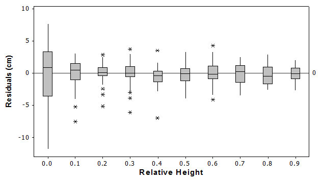
In terms of precision, as measured by the root-mean-square error as a percentage of the mean observed diameter, the corresponding percentages from relative height 0.0 to 0.9 were 10.7, 6.0, 4.8, 5.5, 6.6, 6.5, 8.3, 11.2, 16.4 and 20.6 respectively. These results show low precision at the bottom and top of the stem, being worse at the tip.
The volume-ratio model
For the volume-ratio model (eqn. 8), fixed parameter estimates, corresponding standard error and p-values, the estimates for the residual variance and the variances of the two random effects are displayed in Tab. 4.
Tab. 4 - Parameter estimates, corresponding standard error and p-values for the volume-ratio model (see eqn. 8 in the text). (****): P < 0.0001.
| Parameter | Estimate | Standard error | Pr > |t| |
|---|---|---|---|
| b0 | 0.018 | 0.004 | **** |
| b1 | 0.029 | 0.001 | **** |
| b2 | 10.289 | 0.437 | **** |
| b3 | 5.931 | 0.038 | **** |
| Residual variance | 0.001 | 0.000 | **** |
| Var(u1) | 0.000 | 0.000 | **** |
| Var(u2) | 12.933 | 1.861 | **** |
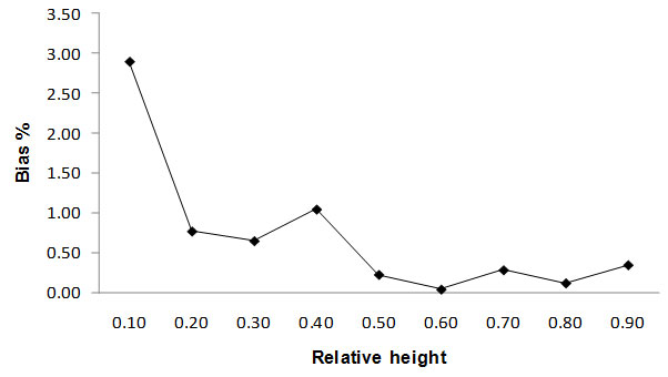
In terms of precision, as estimated by RMSE%, the performance of the volume-ratio model is poorest at the lower portions of the stem and improves towards the top of the tree. RMSE% ranges from a high of 48 % at 0.1 relative heights down to 10 % at the top of the tree. This could be a result of the great variability in bole volume content occurring in the lower portion of the trees due to differences in tree form. The fact that we are interested in predicting volume to upper diameters and RMSE% is below 17 % above 0.5 relative heights makes this lack of fit negligible. The predicted cumulative volumes (inside bark) up the stem with the volume-ratio model were compare to the observed values up to 10 different relative heights. Bias, as percentage of the averaged observed cumulative volume, was computed at each relative height, and may be considered negligible. The greatest lack of accuracy occurred at 0.1 relative height where the bias was 2.89 % (Fig. 2).
Fig. 2 - Bias performance of the volume-ratio model as percentage in the validation data set at different relative heights.
Observed cumulative volume as percentage and superimposed to the corresponding predicted cumulative volume percentages by the fixed effect parameters model and the model including random parameters at different relative heights on three contrasting trees (small, medium and large) of the verification data set were studied. The fixed effect model approximated better the cumulative observed volume between 0.1 and 0.3 relative heights in all three trees. From 0.35 to 0.7 the fixed plus random effects model approximates better the observed cumulative volume percentage and from 0.7 to 0.1 relative heights, at the tip, both models predict similar cumulative volume values.
Cumulative bole volume predictions by the taper and volume-ratio models on verification data set were estimated to three predefined upper stem diameters normally used by forest industries in the study region, employing both the taper and the volume-ratio models. For “saw logs” that upper stem diameter is 14 cm, for “posts” it is 8 cm and for “bars” 4 cm. The predictions were carried out considering both the fixed and the random part of the models. The predicted cumulative volumes were then compared to the corresponding observed cumulative volumes by means of residual analysis. The results are shown in Tab. 5.
Tab. 5 - Goodness-of-fit statistics from the residual analysis performed on the validation data set for cumulative bole volume predictions to three predefined upper stem diameters of 14 cm, 8 cm and 4 cm by the taper and volume-ratio models.
| Goodness- of-fit statistics |
Upper stem diameter | |||||
|---|---|---|---|---|---|---|
| 14 cm | 8 cm | 4 cm | ||||
| Taper | Volume ratio |
Taper | Volume ratio |
Taper | Volume ratio |
|
| MSE | 0.014 | 0.022 | 0.014 | 0.021 | 0.014 | 0.02 |
| RMSE | 0.09 | 0.115 | 0.09 | 0.11 | 0.09 | 0.11 |
| RMSE % | 15.65 | 19.97 | 14.34 | 17.69 | 14.276 | 17.408 |
| Bias | 0.021 | -0.042 | 0.032 | -0.037 | 0.036 | -0.34 |
| Bias % | 3.69 | 7.24 | 5.13 | 5.873 | 5.648 | 5.297 |
| MAD | 0.049 | 0.054 | 0.051 | 0.05 | 0.052 | 0.05 |
| R2 | 0.93 | 0.917 | 0.928 | 0.92 | 0.926 | 0.92 |
When comparing the volume-ratio model to the taper model for their ability to predict merchantable volume to varying merchantability limits using independent data, the taper model proved slightly superior to the volume-ratio model according to most goodness-of-fit statistics. Only for the “bar” product (4 cm upper diameter) the volume-ratio model was slightly better than the taper model in terms of bias and MAD.
Discussion
The selection of the random parameters in the taper models was based on the values of AIC, BIC and -2LL according to the model validation results. The lowest values for the fit statistics above were obtained when the first random coefficient g 1 was added to the intercept term a0 Di1 a2Di, and the second random coefficient g2 was added to the fix parameter β3 accompanying the Z term in the variable-exponent taper model. Both random parameters were statistically significant, demonstrating significant variability in fixed parameters between trees. The correlation coefficient of g1 and g2 was low (0.3) indicating that variation has been accounted by current covariates. Yang et al. ([31]) also incorporated one random parameter into the exponent (b0 parameter) and another for a1 to obtain the best results for several candidate variable-exponent taper equations for lodgepole pine in Alberta, Canada.
Several authors have reported the need to incorporate surrogates of stem form into taper models ([6], [18]) as a means to improve their predictive ability. Garber & Maguire ([11]) and Yang et al. ([31]) found significant functions using D/H ratio (a proxy for tree form) in their taper models for Abies grandis, P. ponderosa and P. contorta in Oregon (the former), and for lodgepole pine in Alberta (the latter). Our results for P. occidentalis shows that D/H ratio was not significant in our model. The effects from this tree form alternative variable may have been captured by the random component on the exponent part of the model.
The location term (i.e., Z) was not significant on its own, although transformed Z functions were statistically significant. The fact that all these terms are functions of the same variable Z may result in the presence of multicollinearity among the independent variables. In our case the predictions were not significantly affected. The inclusion of random effects may have also helped in alleviating autocorrelation problems.
Our taper model had somewhat large prediction bias in the lower portion of the bole (21 % at a relative height Z = 0.1). Higher up the bole, the bias percentage decreases substantially, to values between 5 and 9 %. These results agree with the findings of Garber & Maguire ([11]), but are contrary to what reported by Calama & Montero ([8]). The latter paper found their linear mixed taper model to be less accurate in predicting tree upper stem diameters. However, they developed a linear, rather than nonlinear, mixed model.
Previous studies ([29], [31]) found that including random effects in the modeling process reduces the majority of the autocorrelation among observations. Others report a reduction, but not the complete elimination, of autocorrelation by including random effect parameters ([28]). Our results for P. occidentalis, analogously to what Yang et al. ([31]) found in lodgepole pine, did not reveal obvious trends in the residuals of the variable-exponent equation (Fig. 1), an indication that the inclusion of random effects in the model effectively accounted for the autocorrelation on the observations.
The random effects in the volume-ratio model also take into account the inter-tree variation through the marginal covariance structure. As with the taper model, the random parameters allow individualization of the model fit to each subject tree, accounting for within-tree covariances. The random parameters in the volume-ratio model explain variability in size (total volume) and shape of the volume profile. In this model, the random u 1i term models random slopes in the total volume component of the equation and u 2i models the rate of change of the tree profile.
The improvement of the model fit by the inclusion of the random effect parameters can be verified by the value of the model fit statistics (i.e., AIC, BIC and -2LL) when the random effects are included or not. The model including the two random parameters has the smallest values on the fitting statistics. By excluding the random effect parameters it is assumed that all the cumulative volume observations are independent. In the random effects models, the residuals are measured against the tree-specific predictions, whereas in the fixed effects model, the residuals are measured against the mean tree predictions.
In the present work, we fitted both a variable-exponent taper equation and a total volume-ratio model to P. occidentalis data from La Sierra in the Dominican Republic, using a mixed-effects modeling approach, with the goal of comparing the accuracy and precision of each model based on evaluation criteria using an independent validation data set, and recommend that best model for estimating merchantable volume for different utilization standards for this species in the region. To reach a decision in selecting the best function, caution must be taken. The taper model is superior for predicting merchantable upper stem diameters in terms of the RMSE evaluation. In terms of percent bias, the taper model is superior by 3.55 % and 0.74 % up to 14 and 8 upper stem diameters, respectively; however, the volume-ratio is marginally better by 0.35 % at a 4 cm upper stem diameter.
Unbiased and accurate individual tree volume prediction is useful in determining stand volume in management inventories. Based on this standpoint, the prediction performance by the two models are very similar. However, whenever merchantability standards should change, the taper model would be more flexible to adapt to the new standards and to predict stand volume estimates.
The main concern of these models to predict merchantable volume in P. occidentalis is that they are contrasting with the results found for other pine species when comparing taper and volume ratio to estimate bole volume. In predicting merchantable volume, other studies ([12]) have shown that the total volume-ratio approach have advantages over taper models, because in their development, merchantable cubic-meter volumes and heights are calculated directly. In contrast, taper models are developed using inside diameters which are indirectly related to volume content. Moreover, taper equations are fitted with the purpose of diameter prediction, contrary to the volume-ratio model, which is used to optimize the prediction of volume.
Nonetheless, it is important to point out that, despite the inconsistent results obtained, the methodology proposed in the present work could be useful. The improvement of the predictions by both models (eqn. 8 and eqn. 20) is significant when random effect parameters are used in conjunction with a nonlinear mixed procedure. The random effects allow to individualize the fit of the model to each subject tree and to explain the inter-tree variation by means of the marginal covariance structure. Garber & Maguire ([11]) found that the inclusion of random parameters only was not enough to address autocorrelation in finding variable-exponent taper models for Abies grandis (Douglas ex D. Don) Lindl., Pinus contorta Dougl., and Pinus ponderosa Lawson & C. Lawson. They had to directly model the autocorrelation by adding a variance-covariance matrix in addition to the random parameters.
Conclusions
We fitted a variable-exponent taper equation and a total volume-ratio model to P. occidentalis stem data from La Sierra, Dominican Republic, employing a nonlinear mixed-effects modeling approach. From a financial perspective, the most important part of a tree bole is within the first half of the height. In the Dominican Republic, the most valuable product from P. occidentalis, is the log with a top diameter of 14 cm. After comparing the accuracy and precision of each of the models tested based on robust evaluation criteria in an independent validation data set, we concluded that the bias and precision of the nonlinear mixed taper model is superior to the volume-ratio model for that portion of the bole. Therefore the model represented in eqn. 20 should be used to estimate inside-bark volume content of P. occidentalis, up to the different utilization standards studied, namely top inside diameters of 14 cm, 8 cm and 4 cm.
Due to the fact that the country is mostly mountainous and soils are very fragile for agriculture production, it is clear that forest production should probably be the most important economic activity in the study region and in the country. The soils in the study area are generally poor and shallow, with great extensions of terrain severely degraded and eroded due to deforestation and migratory agriculture. These areas were once populated by our endemic species P. occidentalis, which is the only species in the country capable of prospering in these types of soils. Forest stands not only provide cover to keep soils stable and habitat for wildlife, but they also produce wood and generate rural employment, bringing along important benefits to the social ecosystem.
To maintain and increase P. occidentalis populations, so that the species continues to serve its role as the only one capable of growing in the shallow and infertile soils in the country, as well as continue being the main commercial tree species, it becomes imperative that forest management in the Dominican Republic dispose of the tools developed in the present study. They will permit the prediction of cumulative bole volume to any predefined upper stem diameter on P. occidentalis standing trees, which is essential for estimating current inventory levels and making informed decisions regarding the management of this forest resource. They have allowed the determination of the productive capacity of the three main ecological zones where the species is intensively managed. Further processing of the information on volume content suggest that the amount of inputs committed and silvicultural concepts applied to the management of these forest stands should be more intense in the humid zone and gradually become more extensive from the intermediate to the dry zone.
The productive capacity of the humid zone calls for dedicating its fragile soils to the production of wood, especially P. occidentalis, mixed with plantings of different broadleaf species to help in the protection of water ways and steep terrain. Forest stands of the species in the dry zone have worse shape and lower commercial value; nonetheless, they should be kept under the cover of P. occidentalis. To manage the species, clear cutting as a reproduction method should be avoided because of soil conditions. These shallow and poor soils would favor the occupancy of the terrain by very aggressive shrub species, impeding the successful establishment of regeneration. Establishing new plantations in this zone requires that a big effort be put into site preparation, both in terms of resources and of costs.
Acknowledgements
This investigation was carried out thanks to contributions from FONDOCYT, a research grant from the Dominican Republic government administered by the Ministerio de Educación Superior de Ciencia y Tecnología. We would like to express our gratitude to Ralph D. Nyland, Lianjun Zhang and Edwin H. White. The contribution from the J. William Fulbright Foreign Scholarship Board (FSB) was highly appreciated. Other significant contributors were the Pontificia Universidad Catolica Madre y Maestra, the Graduate Assistantship program at the State University of New York, College of Environmental Science and Forestry and the Collegiate Science and Technology Entry Program (CSTEP) chapter at SUNY_ESF, the Program on Latin America and the Caribbean at Syracuse University, Cooperativa San Jose, Plan Sierra Inc., and PROCARYN.
References
Gscholar
Gscholar
Gscholar
Gscholar
Gscholar
Gscholar
Gscholar
Gscholar
Gscholar
Gscholar
Gscholar
Gscholar
Online | Gscholar
Gscholar
Gscholar
Gscholar
Gscholar
Gscholar
Gscholar
Authors’ Info
Authors’ Affiliation
Vicerrectoría de Investigaciones e Innovación, Pontificia Universidad Católica Madre y Maestra, Autopista Duarte km 1.500, Santiago de los Caballeros (República Dominicana)
State University of New York, College of Environmental Science and Forestry, 1 Forestry Drive, 13210 Syracuse, NY (USA)
Corresponding author
Paper Info
Citation
Bueno-López S, Bevilacqua E (2012). Nonlinear mixed model approaches to estimating merchantable bole volume for Pinus occidentalis. iForest 5: 247-254. - doi: 10.3832/ifor0630-005
Academic Editor
Marco Borghetti
Paper history
Received: Sep 07, 2012
Accepted: Oct 01, 2012
First online: Oct 24, 2012
Publication Date: Oct 30, 2012
Publication Time: 0.77 months
Copyright Information
© SISEF - The Italian Society of Silviculture and Forest Ecology 2012
Open Access
This article is distributed under the terms of the Creative Commons Attribution-Non Commercial 4.0 International (https://creativecommons.org/licenses/by-nc/4.0/), which permits unrestricted use, distribution, and reproduction in any medium, provided you give appropriate credit to the original author(s) and the source, provide a link to the Creative Commons license, and indicate if changes were made.

Web Metrics
Breakdown by View Type
Article Usage
Total Article Views: 63482
(from publication date up to now)
Breakdown by View Type
HTML Page Views: 52581
Abstract Page Views: 3934
PDF Downloads: 5312
Citation/Reference Downloads: 20
XML Downloads: 1635
Web Metrics
Days since publication: 4998
Overall contacts: 63482
Avg. contacts per week: 88.91
Article Citations
Article citations are based on data periodically collected from the Clarivate Web of Science web site
(last update: Mar 2025)
Total number of cites (since 2012): 8
Average cites per year: 0.57
Publication Metrics
by Dimensions ©
Articles citing this article
List of the papers citing this article based on CrossRef Cited-by.
Related Contents
iForest Similar Articles
Research Articles
Modeling compatible taper and stem volume of pure Scots pine stands in Northeastern Turkey
vol. 16, pp. 38-46 (online: 22 January 2023)
Research Articles
Compatible taper-volume models of Quercus variabilis Blume forests in north China
vol. 10, pp. 567-575 (online: 08 May 2017)
Research Articles
Comparative analysis of taper models for Pinus nigra Arn. using terrestrial laser scanner acquired data
vol. 17, pp. 203-212 (online: 22 July 2024)
Research Articles
Analyzing regression models and multi-layer artificial neural network models for estimating taper and tree volume in Crimean pine forests
vol. 17, pp. 36-44 (online: 28 February 2024)
Research Articles
Estimation of stand crown cover using a generalized crown diameter model: application for the analysis of Portuguese cork oak stands stocking evolution
vol. 9, pp. 437-444 (online: 02 December 2015)
Research Articles
Modelling taper and stem volume considering stand density in Eucalyptus grandis and Eucalyptus dunnii
vol. 14, pp. 127-136 (online: 16 March 2021)
Research Articles
The use of tree crown variables in over-bark diameter and volume prediction models
vol. 7, pp. 132-139 (online: 13 January 2014)
Research Articles
Height-diameter models for maritime pine in Portugal: a comparison of basic, generalized and mixed-effects models
vol. 9, pp. 72-78 (online: 11 June 2015)
Research Articles
Modeling stand mortality using Poisson mixture models with mixed-effects
vol. 8, pp. 333-338 (online: 05 September 2014)
Research Articles
Diameter growth prediction for individual Pinus occidentalis Sw. trees
vol. 6, pp. 209-216 (online: 27 May 2013)
iForest Database Search
Search By Author
Search By Keyword
Google Scholar Search
Citing Articles
Search By Author
Search By Keywords
PubMed Search
Search By Author
Search By Keyword


