Three-dimensional forest stand height map production utilizing airborne laser scanning dense point clouds and precise quality evaluation
iForest - Biogeosciences and Forestry, Volume 10, Issue 2, Pages 491-497 (2017)
doi: https://doi.org/10.3832/ifor2039-010
Published: Apr 12, 2017 - Copyright © 2017 SISEF
Research Articles
Abstract
In remote sensing, estimation of the forest stand height is an ever-challenging issue due to the difficulties encountered during the acquisition of data under forest canopies. Stereo optical imaging offers high spatial and spectral resolution; however, the optical correlation is lower in dense forests than in open areas due to an insufficient number of matching points. Therefore, in most cases height information may be missing or faulty. With their long wavelengths of 0.2 to 1.3 m, P-band and L-band synthetic aperture radars are capable of penetrating forest canopies, but their low spatial resolutions restrict the use of single-tree based forest applications. In this study, airborne laser scanning was used as an effective remote sensing technique to produce large-scale maps of forest stand height. This technique produces very high-resolution point clouds and has a high penetration capability that allows for the detection of multiple echoes per laser pulse. A study area with a forest coverage of approximately 60% was selected in Houston, USA, and a three-dimensional color-coded map of forest stands was produced using a normalized digital surface model technique. Rather than being limited to the number of ground control points, the accuracy of the produced map was assessed with a model-to-model approach using terrestrial laser scanning. In the accuracy assessment, the standard deviation was used as the main accuracy indicator in addition to the root mean square error and normalized median absolute deviation. The absolute geo-location accuracy of the generated map was found to be better than 1 cm horizontally and approximately 40 cm in height. Furthermore, the effects of bias and relative standard deviations were determined. The problems encountered during the production of the map, as well as recommended solutions, are also discussed in this paper.
Keywords
Airborne Laser Scanning, Forest Stand Height Map, First Echo, Last Echo, NDSM
Introduction
Over the past few decades, remote sensing techniques that provide three-dimensional (3D) geo-information have become indispensable, particularly for land-related research that analyzes the Earth’s surface. Forest modeling is an area that requires repetitive and costly terrestrial measurements for the creation of an inventory based on single tree-related parameters, such as tree species and their distribution, timber volume and the mean tree height ([10]). Today, information on most of these parameters is obtained by generating 3D height models with remotely sensed data. However, the accuracy of these models remains an open question. This study was partially designed to provide an answer to this question by producing high resolution (25 cm) 3D maps of forest stand height using an effective remote sensing method, namely airborne laser scanning (ALS), and validating the produced map through model-to-model visual and statistical methods. The term 3D height model involves three forms of the main triangular irregular network: a digital surface model (DSM), a digital elevation model (DEM) and a digital terrain model (DTM). In the field of forestry, the DSM demonstrates the canopy of forest at the look-angle of the remote sensing instrument, which includes the X and Y planimetric coordinates and the altitude, Z. DEMs and DTMs also represent bare earth underlying the terrain of forest. Information obtained from a DEM and a DTM are very similar, with the only difference that the DTM provides additional information from hard and soft break-lines and mass points measured with triangular irregular networks.
In flat and open areas, the 3D earth modeling potential of remote-sensing techniques is comparable to that of terrestrial measurements; however, remotely sensed data may be distorted in inclined or forest-covered topographies, due to imaging geometries and limited sensing capabilities. 3D earth modeling that uses passive remote-sensing data derived from space-borne stereo optical imaging and photogrammetry is an operator-dependent semi-automatic process. Even if digital images have very high spatial and spectral resolution, the performance of area-based automatic image-matching algorithms is limited and the operator must visually assign additional matching points to stereo images to improve the accuracy of the final products. Moreover, in dense forest areas, due to low optical correlation, the functionality of the operator becomes even more significant, and due to the lack of details (such as information on constructions, break-lines and fire ways), the operators can only identify a limited number of matching points. Despite the availability of image enhancement methods based on band combinations, such as false color and the normalized difference vegetation index, they are not sufficient to improve the accuracy of the final 3D product to a satisfactory level. On the other hand, synthetic aperture radar (SAR) imagery offers a fully automatic process for generating DSMs and has the advantage of utilizing interferometric synthetic aperture radar (InSAR) technology. However, the long-wavelength penetrative bands (P and L) of SAR do not meet the spatial resolution required for studies of single-tree based forest inventory. The remaining SAR imaging bands (such as S, C and X) fail to penetrate forest canopies and obtain accurate and sufficient information about the underlying bare topography. Due to these limitations, ALS has gradually become the primary technique for mapping forest areas, which offers rapid and highly accurate 3D topographic point clouds that have traditionally not been provided by competing remote sensing technologies ([4], [6]). With its forest penetration capability, achieved through the detection of multiple echoes per laser pulse and dense point clouds, ALS is considered by the scientific community as an effective solution for generating DEMs ([13], [15], [16], [14], [3], [12], [1]).
In this study, a 3D map of forest stand height was created in a forest-covered area located on the main campus of the University of Houston, which utilized a normalized digital surface model (nDSM) alias canopy height model technique. The nDSM is a differential model of the generated DSM and DTM, and it is one of the most reliable and frequently used techniques employed to estimate forest stand heights ([18], [17]). Unlike many studies published in the literature, we identified the most crucial and error-prone points in nDSM generation using dense ALS point clouds, and offer suggestions of how to obtain an accurate model. Moreover, rather than using ground control points (GCP), the accuracy of the generated map was controlled using a model-to-model approach based on the reference nDSM obtained from the terrestrial laser scanning (TLS) data.
This paper is organized as follows: first, the study area and materials are described followed by the methodology section, which gives details about the production of a 3D forest stand height map and accuracy assessment. Later, the generated 3D map and the results of geo-location accuracy assessment are presented, followed by the conclusion.
Materials and methods
Study area and materials
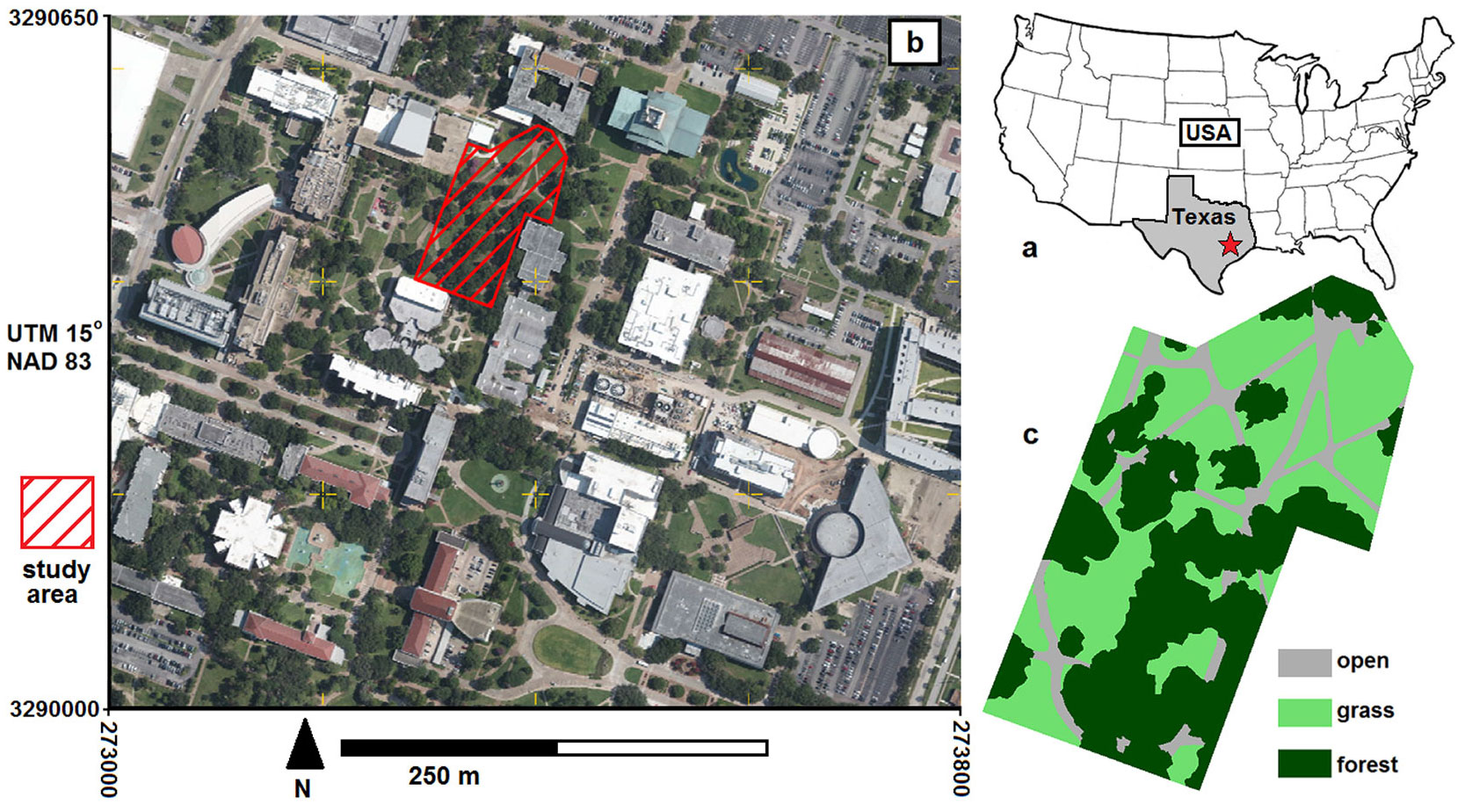
Considering the requirements of this analysis, a forest-covered area located in the main campus of the University of Houston in Texas, USA was chosen as the study area. The study area is 13.000 m2, and it is comprised of three different land classes: open, grass and forest. The orthometric height of the area ranges from 10 to 33 m. Fig. 1 presents the location and land classes of the study area.
Fig. 1 - Location and land classes of the study area: (a) Houston indicated by a red star; (b) sample plot in the main campus of the University of Houston; (c) land classes.
The ALS flights used in this study were completed by the National Center for Airborne Laser Mapping (NCALM) based at the University of Houston. During the flights, the entire area of the main campus (3 × 9 km = 27 km2) was covered and an Optech Gemini airborne laser terrain mapper was used to collect very high-resolution (VHR) point clouds. Due to the intensity of the point clouds, and considering the capability of the computers and software used, the data was divided into 27 tiles of size 1 × 1 km. The TLS measurements were obtained with a Riegl VZ-400® instrument (RIEGL Laser Measurement Systems GmbH, Horn, Austria). The characteristics of the instruments and measurements are listed in Tab. 1.
Tab. 1 - Characteristics of used instruments and measurements.
| Parameter | ALS | TLS |
|---|---|---|
| Instrument | Optech Gemini ALTM | Riegl VZ-400 |
| Date | 23/06/12 | 13/11/13 |
| Point density (m2) | 45 | ≈10000 points ≤ 10m horizontal distance |
| Pulse rate (kHz) | 167 | 300 |
| Wavelength (nm) | 1064 | 1550 |
| Scan frequency (Hz) | 0-70 | n/a |
| Beam divergence (mrad) | 0.25 | 0.35 |
| Field of view (°) | -25 to +25 | 360 horizontal/-40 to +60 vertical |
| Flight altitude (m) | 1000 | n/a |
| Number of returns | 4 | ~Unlimited |
As shown in Tab. 1, the ALS and TLS data were not collected during the same period of the year. However, since the trees in the study area are primarily live oaks, they maintain foliage all year. Therefore, there was no need to collect leaf-on and leaf-off data, and except for some minor differences due to vegetation, we did not expect to see a significant difference between the ALS and TLS data. This was confirmed by visual inspection of the point clouds, which indicated only minimal and smaller changes than observed in the nDSM assessment.
Methodology
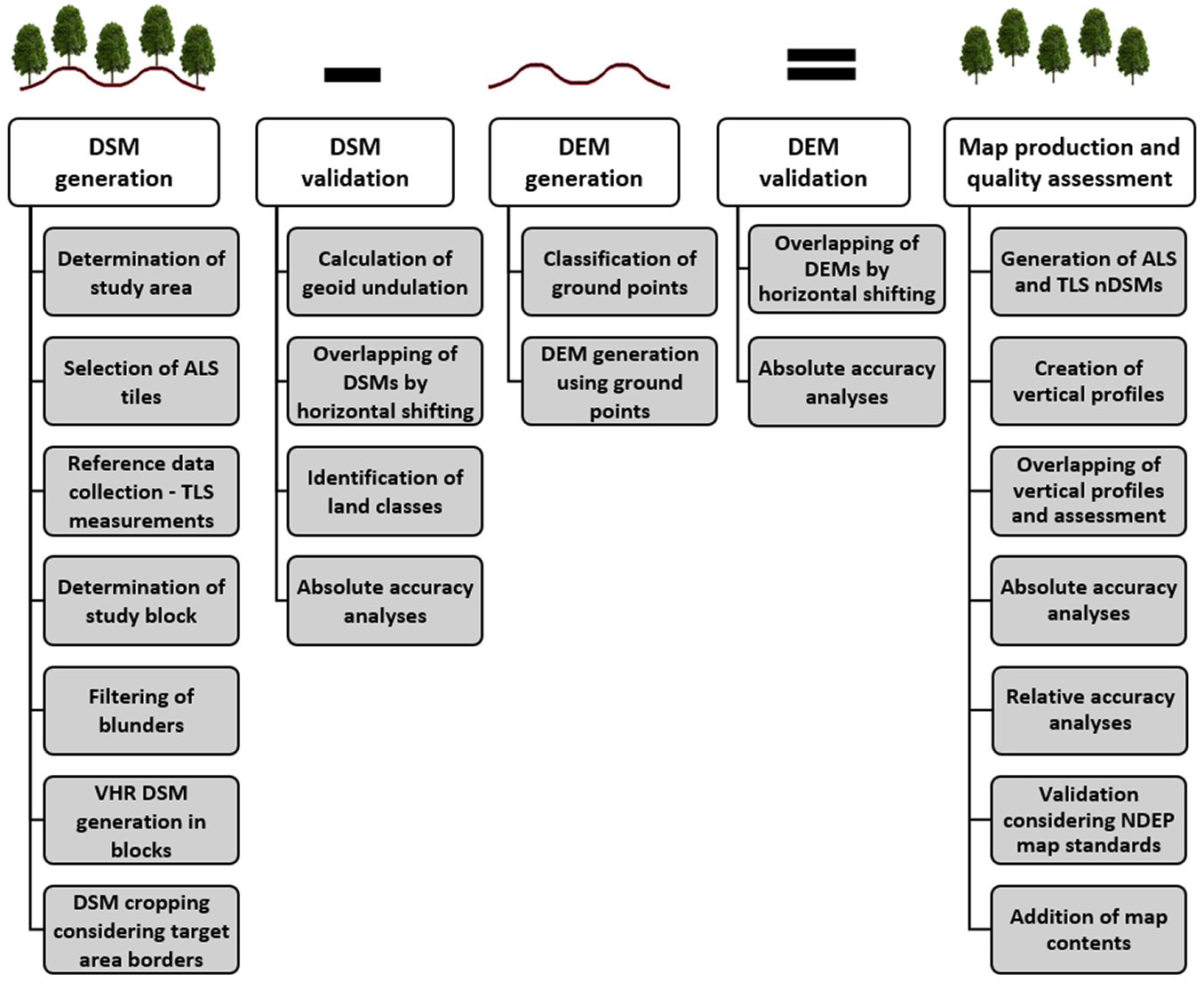
The production of a 3D map of forest stand height, and the assessment of its accuracy, were performed in five main stages, as presented in Fig. 2. Prior to the procedure, NCALM completed the post-processing and calibration of the collected ALS data to render the rough data processable ([5]). In the study, the Terrascan, BLUH (Bundle block adjustment Leibniz University Hannover), Surfer, and LISA software were used to process the ALS data, to generate the DSM, DTM and 3D forest stand maps and to validate the accuracy of the produced models and map. In addition, the Universal Transverse Mercator 15° coordinate system and the North American Datum 1983 were utilized.
Fig. 2 - Stages of the production of a 3D forest stand height map and accuracy assessment.
Generation of the DSM and DTM
In the related ALS data tiles, a study block which covered the study area was identified. The study block had to be wider than the study area over all the border lines to prevent erroneous edges in the DSM and DTM. Due to the lack of sufficient points in the search radius during interpolation, misleading results may be obtained from border lines. To eliminate blunders (isolated and below-ground points) from the point clouds, a three-stage filtering process (Fig. S1a in Supplementary material) was performed. First, the main top and bottom height levels of the area, according to the first and last signal echoes, were determined by drawing vertical profiles. Then, a DSM class was created, and any points that remained between the vertical profile levels were incorporated into this class. This way, any blunder points were excluded from the DSM class. Similar steps were performed to filter the DTM by only using ground points to obtain the most accurate bare topography.
Considering the nature of DSMs and DTMs, and the location geometry of ALS and TLS point clouds, different interpolation techniques were utilized in the generation of the models. During DSM generation with the ALS and TLS data, one problem was related to the presence of perpendicular objects such as trees and walls. When generating a raster DSM by considering the visible surface (top view) of the objects, several points with varying elevations were located in the same pixel due to VHR (Fig. S1b in Supplemetary material). We overcame this issue by using the maximum point elevation within a pixel, rather than averaging, with the help of the data metrics interpolation method. In DTM generation using only ground points, the nearest neighbor interpolation method was applied. After the generation of the DSM and DTM, both the TLS and ALS models for each study block were cropped to fit the pre-determined boundaries of the study area.
Production of a 3D map of forest stand height
A 3D map of forest stand height was produced by calculating the nDSM, which is the differential calculus of a DSM and a DEM or DTM (eqn. 1):
According to the basic principle, when bare topography is removed from the visual surface of the buildings or vegetation, what remains is the elevation of the object (Fig. S1c). In ALS, the nDSM can be summarized as the difference between the surfaces identified with the first and last backscattered echoes of the laser signal. The most significant issue in nDSM generation is the 100% horizontal overlapping of the DSM and DTM that are used. The horizontal offsets (separately in the x and y directions) between these models, which also give the horizontal geo-location accuracy of an ALS, create an insubstantial nDSM due to the calculation of wrong differentials. Due to this effect, the horizontal offsets between the generated DSM and DTM were eliminated by shifting based on an area matching cross-correlation.
Accuracy of the produced map
Accuracy assessment is one of the major processes in the production of a map created from remotely sensed data. This assessment can be performed by various techniques, which can determine the usefulness of the map according to pre-determined accuracy standards. The accuracy of 3D products generated using remotely sensed data was validated mainly by point-based comparison approaches that utilize GCPs collected by Global Navigation Satellite Systems (GNSS) measurements. However, and particularly for rough terrains, a limited number of GCPs is not adequate to assess the accuracy of 3D raster maps generated with VHR ALS point clouds, which can result in misleading numerical results and interpretations. To achieve the most reliable results, we aimed to include all the pixels of an ALS raster map in the accuracy calculation. In this context, the most eligible technique is the model-to-model comparison of the test data with reference data ([11], [9]). When selecting the reference data, the following criteria should be fulfilled: (i) the reference data should cover the whole study area without any remarkable distortions; (ii) the resolution of the reference data has to be equal to or higher than the test data; and (iii) the absolute accuracy of the reference data should be superior to that of the test data. Considering particularly conditions (ii) and (iii), and the available mapping technologies, in the accuracy validation of a generated ALS 3D map, the TLS data was chosen as the most appropriate. The TLS point clouds were collected from four independent stations and their geo-reference adjusted with a minimum of three external targets. The precise locations of these targets were then determined through long (> 1 hour) static surveys that used dual frequency GNSS receivers. TLS is a multi-return instrument and is therefore able to obtain measurements from all levels of the vegetation canopy, with an average point spacing of 1 cm. The dense TLS sampling and multi-return capability (sometimes > 5 returns per outgoing pulse) allowed to model the top of the canopy well with 5 mm absolute geo-location accuracy and 3 mm relative accuracy within a range of 100 m.
During the analyses, geoid undulation was applied at 27.284 m according to Geoid 12A, and the vertical geo-location accuracies were determined from the absolute standard deviation (SZ) of the height differences (eqn. 2):
To estimate the effects of terrain tilt on SZ, a terrain tilt function was also calculated as follows (eqn. 3):
where SZtt is SZ expressed as function of terrain tilt, tan (α) is the tangent of terrain tilt and b is a multiplicative factor.
In addition to the main indicator SZ, the root mean square error (RMSZ - eqn. 4) and the normalized median absolute elevation (NMAD) derived from median absolute deviation (MAD - eqn. 6 and eqn. 7) were used in the assessment of the absolute accuracy. In eqn. 6, i is the median of the height discrepancies between the reference and test data. SZ represents the average, while the RMSZ is influenced by the systematic bias. The influence of systematic bias is equal to the arithmetic mean of the height differences (µ) between the reference and test data. eqn. 5 presents the relation between the SZ and RMSZ based on bias. Due to its squared-sum nature, the SZ is strongly affected by larger discrepancies. The NMAD is based on the median, and therefore it does not change significantly if the error frequency does not correspond to a normal (symmetric) distribution. For a normal distribution, the SZ and NMAD should be almost identical ([7]), whereas in asymmetrical cases, the error frequency description of the NMAD is superior to the SZ. Contrary to the RMSZ, it is possible to validate and identify outliers using the SZ and NMAD. In the analysis, any systematic bias that was a linear function of Z between the test and reference models was determined via linear regression, where we calculated the vertical shift and scale differences. The absolute vertical accuracies were calculated with the systematic bias eliminated (eqn. 4 to eqn. 7).
The interior integrity of the produced map was determined by calculating the relative standard deviation (RSZ) based on the relationship between neighboring pixels (eqn. 8). The RSZ was estimated by separately grouping pixels and considering the distance of the current point to a reference point for both height differences dZ [difference of Z(reference) - Z(compared point in the distance group)], when they were available (eqn. 8):
where Dl<D<Du. Hence, the height discrepancies of neighboring points were compared, and the dependency (correlation of dZ) was checked. In this way, local random errors and random errors could be separated. In the case where differences were found in the independent heights (correlation = 0), RSZ was identical to SZ, and if the correlation coefficient was 1.0, RSZ would be zero. Under normal conditions, the RSZ had a value between zero and SZ. In extreme cases of a negative correlation, the RSZ may be larger than SZ. In normal conditions, the RSZ of active remote sensing systems such as radars and lasers are superior to their absolute accuracies ([8], [9], [2]). In eqn. 8, D represents the distance groups (the distance of the current point to a reference point, when height differences are available for both) and Dl and Du are the lower and upper distance limits, respectively. In this study, the distance groups varied from the 1st to the 10th pixel (0.25 to 2.5 m, considering the 0.25 m pixel size of the reference TLS data), since for each pixel 10 neighboring pixels were used in the calculation. The term nx is the number of point combinations in the distance group, and n is the total number of differences between the reference and actual values. The term nx is multiplied by a factor of 2 in order to normalize RSZ to the size of SZ. If the height differences of the points in a distance group are independent, corresponding to error propagation, the RMS will be √2 times larger than SZ. This is represented by 2 × nx.
Results
Generated models and maps
Fig. 3 presents the DSM and DTM generated with ALS using a color scale for height. Only ground points were used in DTM generation and all non-terrain objects were eliminated. The last echo of a laser signal may not always return from the bare earth depending on the number of returns of the laser scanner. Sometimes, the last echo may return from a level of understory trees or low vegetation such as bracken or grass. This is why the point density is expected to be lower in the ground layer. As a consequence, the influence of interpolation can be seen more clearly in the DTM due to the use of further points. The solution for increasing the point density on the ground layer is to use a laser scanner which enables more returns of the signal; however, this increases the point density in all layers that results in large amounts of unnecessary data.
Fig. 3 - Models generated with ALS: (a) DSM; (b) DTM.
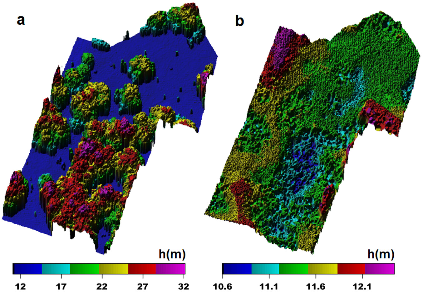
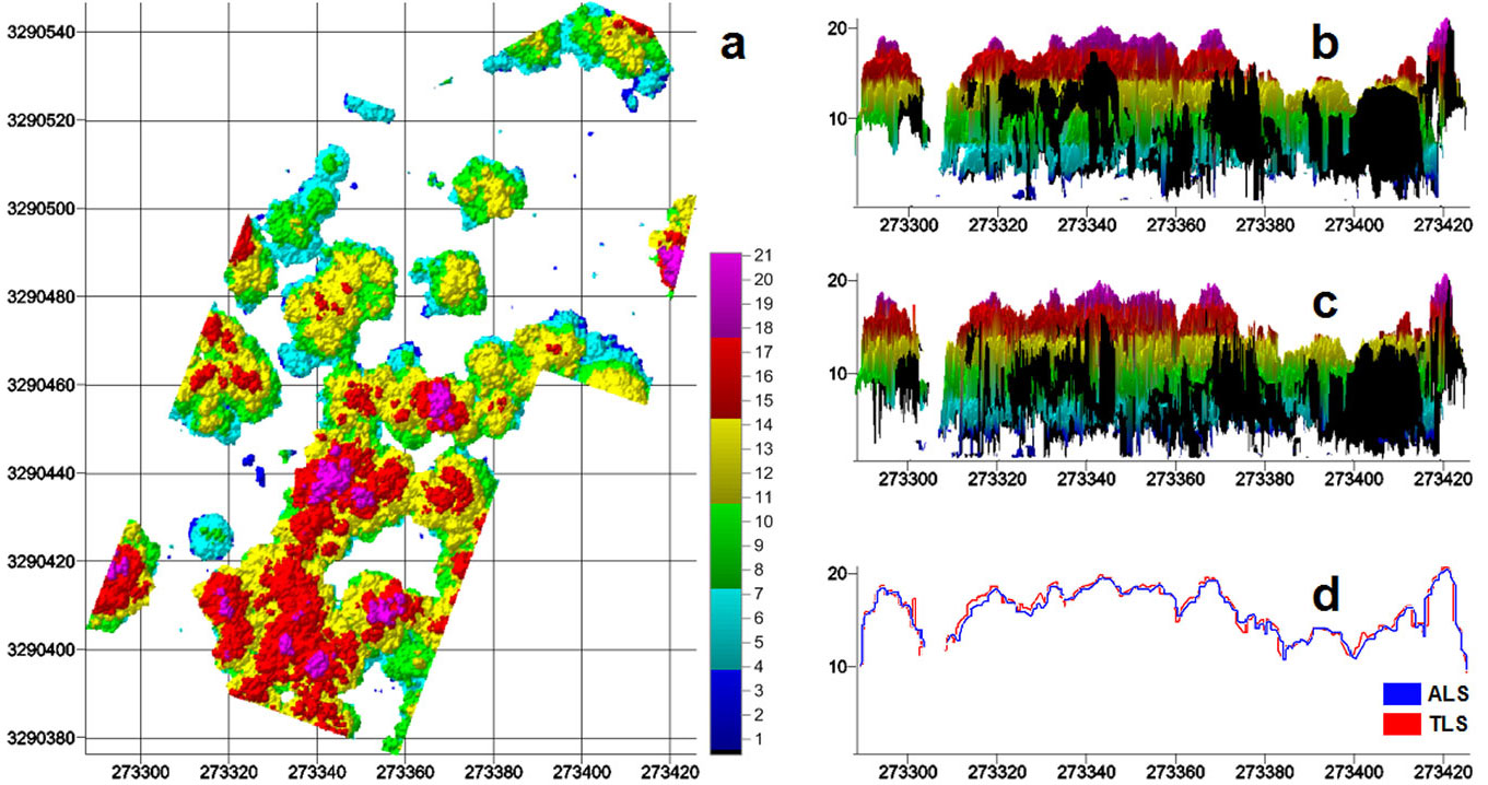
Fig. 4 illustrates the produced 3D map of forest stand height using a color-coded scale. For the comparison of the produced map with the reference TLS map, the vertical profiles of the ALS and TLS maps are plotted in the Y direction. It is clear that the produced map matches the reference map in almost every part of the canopy except for small disparities due to vegetation growth. In addition, the ALS map has a systematic tendency to estimate the heights of the crowns and the terrain to slightly lower values than are present in the reference TLS map. The amount of this systematic bias was determined and eliminated in the vertical accuracy assessment. In the interpretation of the data, the up-down and down-up scanning views of ALS and TLS should not be overlooked.
Fig. 4 - Comparison of the produced (ALS) map with the reference (TLS) map: (a) the ALS map; (b) vertical profile of the ALS map in the Y direction; (c) vertical profile of the TLS map in the Y direction; (d) comparison of the vertical profiles.
Accuracy of the generated models and map
Tab. 2 presents the absolute horizontal and vertical accuracies of the produced map in relation to the reference map including standard deviation of X and Y discrepancies (SX, SY), SZ, SZ as function of terrain tilt (SZtt), RMSZ and NMAD. The horizontal accuracy of the produced map is very high, and ranges from 0 to 9 cm. The vertical accuracies are given with and without the effects of systematic bias. The systematic biases varied for the DSM, DTM and nDSM comparisons between the ALS and TLS due to using different interpolation techniques in their generation. The elimination of systematic bias was found to have a significant effect on the absolute vertical accuracy, particularly on the excluded points, which resulted in a height difference >1 m between the produced map and the reference map. The DSM and DTM assessment system, BLUH, only compared data that were available in both models, and if the test data corresponded to a gap in the reference data, this pixel was identified and excluded. As expected, in the produced map (nDSM), the vertical accuracy was lower compared to the results of the DSM and DTM due to the map only covering the forest layer and ignoring open and flat areas. In this study, the accuracy of the ALS data was evaluated according to the standards developed by the American Society for Photogrammetry and Remote Sensing ([2]) for large-scale maps based on contour interval (Tab. 3). The produced map almost fulfills the horizontal and vertical geo-location requirements for 1/2000-scaled topographic maps, which means that it can be presented at this scale.
Tab. 2 - Absolute horizontal, absolute vertical accuracies and percentage of excluded points.
| Reference model |
Tested model |
SX (cm) |
SY (cm) |
Bias (m) |
RMSZ (m) |
SZ | NMAD | SZtt | Excluded points (%) |
|---|---|---|---|---|---|---|---|---|---|
| TLS DSM (0.25m) | ALS DSM (0.25m) | 0.31 | -0.22 | -0.48 | 0.498 | 0.149 | 0.071 | 0.461 + 0.16·tan(α) | 10.14 |
| 0.00 | 0.179 | 0.179 | 0.085 | 0.109 + 0.18·tan(α) | 7.72 | ||||
| TLS DTM (0.25m) | ALS DTM (0.25m) | 8.02 | 9.61 | -0.23 | 0.270 | 0.135 | 0.134 | 0.270 + 0.35·tan(α) | 0.02 |
| 0.00 | 0.135 | 0.135 | 0.132 | 0.182 + 0.35·tan(α) | 0.01 | ||||
| TLS nDSM (0.25m) | ALS nDSM (0.25m) | 0.01 | 0.89 | -0.36 | 0.521 | 0.376 | 0.368 | 0.429 + 0.17·tan(α) | 29.94 |
| 0.00 | 0.422 | 0.422 | 0.419 | 0.415 | 21.27 |
Tab. 3 - Map accuracy requirements according to map scale and contour interval ([2]). (1): 95% confidence level (1.96×RMS).
| Map scale | Contour interval (m) |
Horizontal | Vertical | ||
|---|---|---|---|---|---|
| RMS (cm) |
Accuracy 1 (cm) |
RMS (cm) |
Accuracy 1 (cm) |
||
| 1:500 | 0.5 | 0.28 | 0.55 | 4.60 | 9.10 |
| 1:1000 | 1 | 0.56 | 1.10 | 9.25 | 18.2 |
| 1:2000 | 2 | 1.12 | 2.20 | 18.5 | 36.3 |
| 1:5000 | 5 | 2.79 | 5.47 | 46.3 | 90.8 |
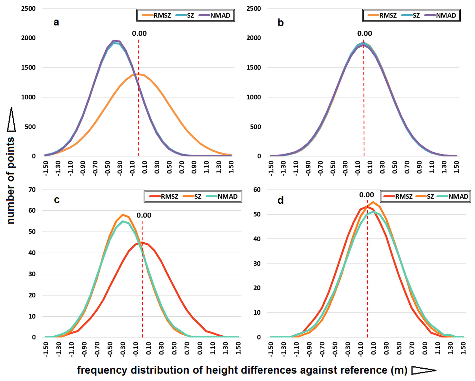
The frequency distribution of height differences between the produced map and the reference map is shown in Fig. 5a and Fig. 5b with and without the effect of systematic bias, respectively. The height differences are normally (symmetrically) distributed for all accuracy indicators. In Fig. 5a, the SZ and NMAD clearly demonstrate the effects of bias. With the elimination of the systematic bias, all accuracy indicators are almost at the same level. Fig. 5c and Fig. 5d show the frequency distribution of height differences in zero slope points with and without systematic bias, respectively. A comparison of Fig. 5a and Fig. 5c gives the negative influence of terrain tilt. Without the effects of bias, the modes of all accuracy indicators are at similar levels, which are close to zero.
Fig. 5 - Frequency distribution of height differences between the produced map and the reference map with and without systematic bias according to (a, b) terrain slope and (c, d) zero slope.
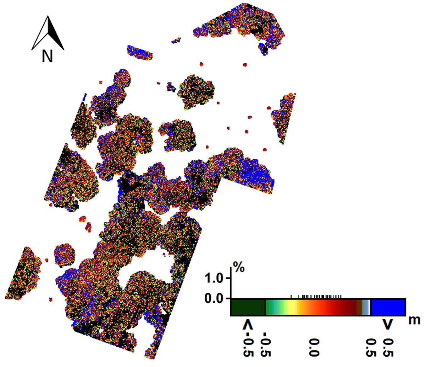
The accuracies of the produced map and the frequency distribution of heights are given above; however, the locations of these differences also need to be presented on the map. Therefore, a differential nDSM (Fig. 6) was generated to demonstrate the color-coded locations of differences. In the differential model, the threshold was determined as |50| cm for this product, and height differences were divided into three classes: from -50 to 50 cm; below -50 cm; and above 50 cm. Tab. 4 shows the RSZ of the produced map with and without systematic bias. As mentioned earlier, the RSZ was separately calculated for each distance group of neighboring pixels. This way, the height discrepancies of the neighboring points are compared. As shown in Tab. 4, the RSZ varies between 30 and 40 cm, and it is not larger than the SZ, which means that normal conditions apply. The analysis of the trends of RSZ with and without systematic bias indicated that there were no outliers.
Fig. 6 - Differential nDSM including the color scale of height discrepancies (dark green = below -50 cm; blue = above 50 cm; changing colors = from -50 to +50 cm).
Tab. 4 - Relative standard deviations of produced map with and without bias.
| Number of neighbored pixel |
RSZ with BIAS (m) |
RSZ without BIAS (m) |
|---|---|---|
| 1 | .29 | .33 |
| 2 | .33 | .37 |
| 3 | .34 | .39 |
| 4 | .35 | .40 |
| 5 | .35 | .40 |
| 6 | .36 | .41 |
| 7 | .36 | .41 |
| 8 | .36 | .41 |
| 9 | .36 | .41 |
| 10 | .37 | .41 |
Conclusions
In this study, a 3D map of forest stand height was produced using an effective remote sensing method, ALS. This method offers very high-resolution point clouds and can penetrate forest canopy through the detection of multiple echoes per each laser pulse. A suitable study area with a forest coverage of approximately 60% was selected at the University of Houston. The geo-location accuracies of the produced map were analyzed using a model-to-model, rather than a point-based, approach. The TLS data were deemed convenient as the reference data for calculations. SZ was chosen as the main accuracy indicator in addition to the use of the RMSZ and NMAD for the prediction of absolute accuracy. Furthermore, the effects of terrain tilt on the accuracy of the results were evaluated. The results demonstrate that the geo-location accuracy of the produced map is better than 1 cm horizontally and approximately 40 cm in height. According to the ASPRS standards, this accuracy is sufficient for the production of a 1/2000 scale topographic map. Another important result was about the significant effects of systematic bias on accuracy. The differences between the produced map and the reference map in terms of height frequencies were normally distributed with no outliers. The locations and the magnitudes of the height discrepancies were shown using a differential nDSM. In addition, as expected for active remote sensing systems under normal conditions, the RSZ was superior to the absolute standard deviation.
Overall, the results clearly demonstrate that ALS data can be effectively used to produce 3D maps of forest stand height up to the 1/2000 scale.
Acknowledgements
We would like to thank the Scientific and Technological Research Council of Turkey, University of Houston, NCALM and Bulent Ecevit University. We would also like to thank Dr. Karsten Jacobsen, who supported us with the software BLUH.
References
Gscholar
Gscholar
Online | Gscholar
Online | Gscholar
Authors’ Info
Authors’ Affiliation
Department of Geomatics Engineering, Bulent Ecevit University, 67100 Zonguldak (Turkey)
Department of Forest Engineering, Faculty of Forestry, Bartin University, 74100 Bartin (Turkey)
Corresponding author
Paper Info
Citation
Sefercik UG, Atesoglu A (2017). Three-dimensional forest stand height map production utilizing airborne laser scanning dense point clouds and precise quality evaluation. iForest 10: 491-497. - doi: 10.3832/ifor2039-010
Academic Editor
Piermaria Corona
Paper history
Received: Mar 03, 2016
Accepted: Jan 27, 2017
First online: Apr 12, 2017
Publication Date: Apr 30, 2017
Publication Time: 2.50 months
Copyright Information
© SISEF - The Italian Society of Silviculture and Forest Ecology 2017
Open Access
This article is distributed under the terms of the Creative Commons Attribution-Non Commercial 4.0 International (https://creativecommons.org/licenses/by-nc/4.0/), which permits unrestricted use, distribution, and reproduction in any medium, provided you give appropriate credit to the original author(s) and the source, provide a link to the Creative Commons license, and indicate if changes were made.

Web Metrics
Breakdown by View Type
Article Usage
Total Article Views: 50177
(from publication date up to now)
Breakdown by View Type
HTML Page Views: 41043
Abstract Page Views: 3622
PDF Downloads: 4110
Citation/Reference Downloads: 17
XML Downloads: 1385
Web Metrics
Days since publication: 3386
Overall contacts: 50177
Avg. contacts per week: 103.73
Article Citations
Article citations are based on data periodically collected from the Clarivate Web of Science web site
(last update: Mar 2025)
Total number of cites (since 2017): 6
Average cites per year: 0.67
Publication Metrics
by Dimensions ©
Articles citing this article
List of the papers citing this article based on CrossRef Cited-by.
Related Contents
iForest Similar Articles
Research Articles
Determining basic forest stand characteristics using airborne laser scanning in mixed forest stands of Central Europe
vol. 11, pp. 181-188 (online: 19 February 2018)
Technical Advances
Forest stand height determination from low point density airborne laser scanning data in Roznava Forest enterprise zone (Slovakia)
vol. 6, pp. 48-54 (online: 21 January 2013)
Research Articles
Integrating area-based and individual tree detection approaches for estimating tree volume in plantation inventory using aerial image and airborne laser scanning data
vol. 10, pp. 296-302 (online: 15 December 2016)
Review Papers
Accuracy of determining specific parameters of the urban forest using remote sensing
vol. 12, pp. 498-510 (online: 02 December 2019)
Research Articles
Are we ready for a National Forest Information System? State of the art of forest maps and airborne laser scanning data availability in Italy
vol. 14, pp. 144-154 (online: 23 March 2021)
Research Articles
Integration of tree allometry rules to treetops detection and tree crowns delineation using airborne lidar data
vol. 10, pp. 459-467 (online: 04 April 2017)
Technical Reports
Remote sensing of american maple in alluvial forests: a case study in an island complex of the Loire valley (France)
vol. 13, pp. 409-416 (online: 16 September 2020)
Research Articles
Comparing image-based point clouds and airborne laser scanning data for estimating forest heights
vol. 10, pp. 273-280 (online: 23 February 2017)
Review Papers
Remote sensing-supported vegetation parameters for regional climate models: a brief review
vol. 3, pp. 98-101 (online: 15 July 2010)
Research Articles
Identification and characterization of gaps and roads in the Amazon rainforest with LiDAR data
vol. 17, pp. 229-235 (online: 03 August 2024)
iForest Database Search
Search By Author
Search By Keyword
Google Scholar Search
Citing Articles
Search By Author
Search By Keywords
PubMed Search
Search By Author
Search By Keyword


