Determining basic forest stand characteristics using airborne laser scanning in mixed forest stands of Central Europe
iForest - Biogeosciences and Forestry, Volume 11, Issue 1, Pages 181-188 (2018)
doi: https://doi.org/10.3832/ifor2520-010
Published: Feb 19, 2018 - Copyright © 2018 SISEF
Research Articles
Abstract
This study focused on the derivation of basic stand characteristics from airborne laser scanning (ALS) data, aiming to elucidate which characteristics (mean height and diameter, dominant height and diameter) are best approximated by the variables obtained using ALS data. The height of trees of different species in four permanent plots located in the Slovak Republic was derived from the normalised digital surface model (nDSM) representing the canopy surface, using an automatic approach to identify local maxima (individual treetops). Tree identification was carried out using four different spatial resolutions of the nDSM (0.5 m, 1.0 m, 1.5 m, and 2.0 m) and the number of trees identified was compared with reference data obtained from field measurements. The highest percentage of tree detection (69-75%) was observed at the spatial resolutions of 1.0 and 1.5 m. Absolute differences of tree height between reference and ALS datasets ranged from 0 to 36% at all spatial resolutions. The smallest difference in mean height was obtained using the higher spatial resolution (0.5 m), while the smallest difference in the dominant height of the relative number of thickest trees (h10% and h20%) was observed using the lower spatial resolution (2 m). The same trends also apply to diameters. The average errors at resolution of 1.0 and 1.5 m was 8.7%, 5.9% and 9.7% for mean height, h20% and h10%, respectively. ALS-derived diameters (obtained using regression models from reference data and ALS-derived individual height as predictor) showed absolute errors in the range 0-48% at all spatial resolutions. The deviation in mean diameter at a resolution of 0.5 m ranged from -12.1% to 15.3%.
Keywords
Forestry, Airborne Laser Scanning, Mixed Forest, Height of Forest Stand, Diameter of Forest Stand
Introduction
Quantitative information on stand and tree characteristics, such as the number of trees, height, diameter and volume, is basic to make decisions in forest management ([35], [34]). Data on these characteristics and the forest environment can be obtained using traditional (ground) methods or by remote sensing (RS) techniques ([25], [36]). Currently, ground methods are being more and more replaced by automated data collection based on aerial and satellite images or data from airborne laser scanning (ALS - [15]), thanks to their cost and time efficiency. Photogrammetry methods have been applied to forest mapping for long time, and ground geodetic methods were used only in cases where details were not achievable from orthophotos ([36]). The main advantage of ALS lies in the 3D point cloud obtainable by laser impulses passing through tree crowns ([26]). The development of ALS started during the 1970s and 1980s, and suitable scanning methods were derived during the 1990s. The first applications were topographically oriented. Since then, the development of this technology was fast and ALS are currently used in a wide range of applications, including forestry ([2], [13]). The history of the development and use of ALS in forestry are described in Hyyppä et al. ([6]).
The number of trees and their position on the ground is the most important information achievable from ALS data ([27]). The best results are obtained for dominant trees in the canopy layer: in younger stands and trees in the understorey layer, the number of trees is likely to be underestimated ([21], [5]). A multitude of algorithms and procedures for the identification of individual trees have been proposed in the literature ([8], [10], [11], [28], [32]), which can be grouped in two basic approaches: (i) an area-based approach where forest characteristics are estimated using statistical analyses and models between ALS data and terrestrial measurements; and (ii) an individual tree-based approach whereby individual trees are identified from ALS data, visually or by segmentation processes, and dendrometric parameters are extracted for individual trees ([2], [10], [32]). Accuracy of tree detection is usually higher in conifer stands as compared to stands with deciduous trees ([27]). The correct identification of trees and their number is critical to derive further tree and stand characteristics such as height, diameter at breast height (DBH), volume, biomass, etc. ([28], [31]).
Tree height can be directly obtained from ALS data, though it is often underestimated as tree tops do not always reflect the laser impulses, particularly when a low scanning density is used ([17]). On the other hand, tree height is likely to be overestimated in terrain with great slopes and mountain areas ([2]). In order to accurately assess tree height a suitable density of the point cloud is crucial. Takahashi et al. ([30]) recommended a density of at least 8.8 points per m2 in order to achieve a deviation in height estimates lower than 1 m; Andersen et al. ([1]) reported a minimum number of 4-5 points per m2 to correctly identify the tree tops. With old trees having large crowns, a density of two points per m2 is assumed to be sufficient. Nevertheless, if quality results are to be achieved, 10 or more points per m2 are appropriate for data extraction ([10]).
While tree height and crown diameter can be measured directly from ALS data, DBH and volume have to be derived following known relations ([2], [6]). The DBH can be derived by regression analysis using data measured on the ground ([12], [34]) or formulas derived from existing relationships ([15], [16]). One of the methods commonly used to derive tree DBH from ALS data is its calculation using the derived height and crown size as predictors. However, crown sizes automatically obtained from ALS data are often inaccurate, and therefore their use may lead to a fairly significant degree of uncertainty ([10]). Moreover, the drawback of a large number of derived relationships between tree height and diameter is their strict dependence on specific stand structures and local natural conditions.
In this paper an automatic approach for tree identification and estimation of their dendrometric characteristics is presented, aimed at assessing the influence of spatial resolution of ALS data on both tree identification and the determination of tree parameters. Tree identification was done at four different spatial resolutions. The height of trees was determined automatically from the normalised digital surface model (nDSM) obtained from ALS data. Determination of the tree diameter was obtained by regression analysis based on reference (ground) data. ALS-derived tree parameters were then compared to those calculated from reference data obtained from field measurements. The aim was to find dependencies between ALS-derived tree parameters and the spatial resolution of ALS data.
Methodology
Study area
The study area is a part of the University Forest Enterprise at the Technical University in Zvolen, Slovak Republic (48° 37′ N, 19° 04′ - Fig. 1). The whole territory is a part of an ancient eruptive region (Kremnické vrchy) characterized by a broken relief with different climatic characteristics.
Fig. 1 - Geographic location of the four permanent research plots in the University Forest Enterprise of the Technical University in Zvolen (Slovak Republic).
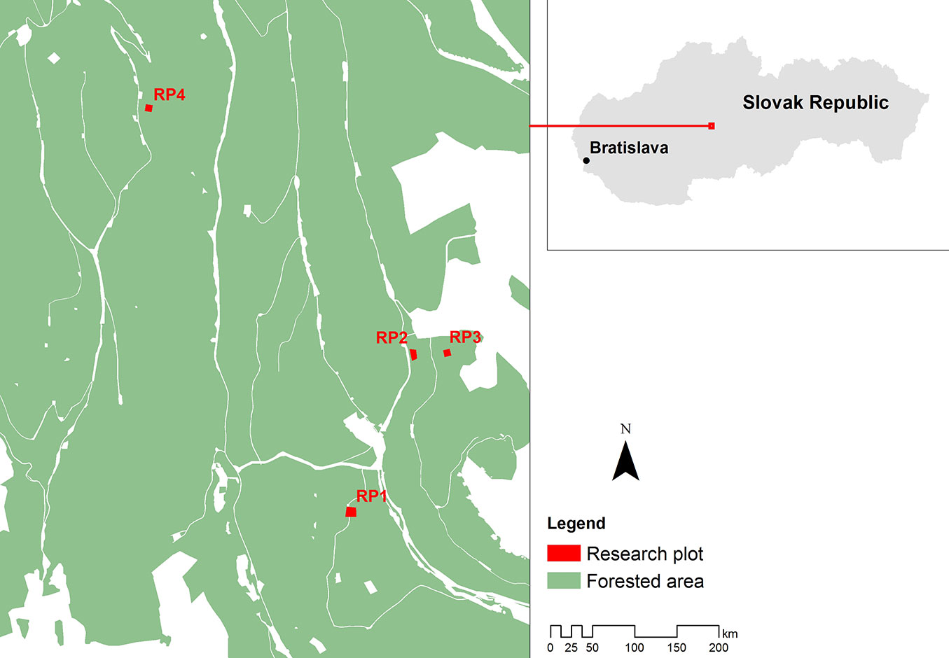
The study area contained four permament research plots (RP). RP 1 is located in the northern part of stand 350a. The stand is 105 years old, with an area of 0.5 ha and average slope of 23.3%. The most abundant tree species in RP1 is the European beach (Fagus sylvatica L.), representing almost 40% of standing trees. The share of broadleaved and coniferous trees was 92% and 8%, respectively. RP2 (area = 0.3 ha; average slope = 34.6%; stand age = 100 years) is located in the northern part of stand 314, where European silver fir (Abies alba Mill.) is the most abundant tree species (almost 36% of extant trees). The share between broadleaved and coniferous trees was 57% and 43%, respectively. RP3 (northern part of the stand 304b) has stand age of 90 years, an area of 0.25 ha and average slope of 7.1%. European silver fir and Norway spruce (Picea abies Karst.) were the most abundant species (31% and 30%, respectively), with a share of broadleaved trees of 39%. RP4 is located in the central part of stand 518a (150 years old; area = 0.25 ha; average slope = 23.7%). European beech represents 100% of trees here.
Terrain slope was calculated from the digital terrain model (DTM - see below), while the tree composition was obtained by field measurement. Stand age was obtained from the Forest management plan (see [24] and [3] for more details).
Data
ALS data were provided by a vendor in September 2011. The airborne laser scanner employed was a Riegl L-680i® (Riegl Laser Measurement Systems Gmbh, Horn, Austria), with a flight altitude of 700 m and a 50° field of view, PRR 320 kHz and SR 122 Hz. The resulting RMSE of the absolute data position was 0.047 m. The ALS data provided by the vendor were recorded as ground points and non-ground points (representing vegetation, buildings and other objects). ALS data were processed using the software Microstation V8 with the application TerraScan® by the vendor. The main characteristics of the ALS dataset are reported in Tab. 1. The images used for the manual vectorisation of data were also taken during the flight. The camera employed was a Vexcel UltraCamX® (Vexcel Imaging GmbH, Graz, Austria). GrafNav® (Waypoint, Novatel Inc., Calgary, Canada) and AEROoffice® (IGI mbh, Kreuztal, Germany) software were used for data processing. The image orthorectification was performed at the Department of Forest Management and Geodesy (Technical University in Zvolen, Slovak Republic) using the Inpho® software package (Trimble Geospatial Inc., Sunnyvale, CA, USA). The spatial resolution of the orthophotos was 10 cm.
Tab. 1 - Characteristics of the ALS dataset used for tree identification. (RP): research plot; (DSM): digital surface model; (DTM): digital terrain model.
| Parameter | RP1 | RP2 | RP3 | RP4 | ||||
|---|---|---|---|---|---|---|---|---|
| DSM | DTM | DSM | DTM | DSM | DTM | DSM | DTM | |
| No. of points | 111,353 | 36,897 | 119,823 | 22,419 | 106,902 | 14,859 | 121,522 | 25,294 |
| Minimum Z | 382.340 | 382.34 | 385.280 | 385.28 | 421.390 | 421.39 | 609.95 | 609.95 |
| Maximum Z | 435.05 | 405.18 | 439.530 | 402.8 | 459.050 | 424.17 | 657.04 | 623.79 |
| Average point distance [m] |
0.218 | 0.378 | 0.165 | 0.38 | 0.153 | 0.407 | 0.144 | 0.319 |
Field measurement was conducted in each RP. The position of the RP centre was measured using the Global Navigation Satellite System (GNSS) and further corrected by visual analysis based on the normalized digital surface models. After manual correction, a sub-meter horizontal accuracy was expected for all RP. The position, height and diameter at breast height (DBH) of each tree were measured using FieldMap® (IFER Ltd., Jilove u Prahy, Czech Republic). The position in the storey of each tree was also identified. Depending on the covering exerted by tree crowns in the upper canopy layer, a metric was set for the potential visibility of each tree from above (i.e., its visibility by the ortophotos). Trees were classified in two categories: (0) no visibility (tree crown covered from above by other trees); (1) visible trees (tree crown not or partially covered from above). Most trees classified as category (0) were supressed trees in the understorey and not visible from orthophotos. Therefore, only trees classified in category (1) were taken into consideration for further analyses.
ALS data processing
ALS data were processed in the OPALS environment ([18]) that was developed at the Institute of Photogrammetry and Remote Sensing, Dept. of Geodesy and Geoinformation at the University of Technology in Vienna (Austria). The margin of each plot was extended by 15 m to eliminate the errors occurring at the plot margin during data processing. This step ensured the integrity of crowns partly falling outside the RP. The process of tree identification was carried out at spatial resolutions ranging from 0.5 to 2 m with a 0.5 m step. The required spatial resolution was defined using the Cell module in OPALS. The Cell module derives models through accumulating the selected attribute parameters. Laser height was used as the attribute and the highest attribute value was used as the “max” parameter. Subsequently, two digital surface models (DSM) were created with a grid equal to the spatial resolution that was set in the previous step. To enable DSM creation, non-ground points were imported into OPALS and stored in the OPALS data manager (ODM - for more information see [19] and [14]). The first DSM was created using the interpolation method of moving planes with the quadrant selection mode. Hereby a grid dataset was created representing the sigma 0 of the grid post adjustment (i.e., the standard deviation of the unit weight observation). The second DSM was created by the aggregation of the max values for laser height, which was set as an attribute. The final DSM was created by combining these two DSMs and the sigma 0 raster layer using the Algebra module. The Algebra module is designed to derive a new grid dataset by combining multiple input grid datasets ([18]). The logical condition is explained by the relation (eqn. 1):
where r[0] is the DSM derived by the moving planes interpolation method; r[1] is the DSM with an aggregated parameter; r[2] is the raster layer representing sigma 0; and d is the defined value.
The DTM was derived using the moving planes interpolation method with the quadrant selection mode. The grid has the same resolution as the DSM. Interpolation was made from the ground points stored in the ODM. The normalised DSM (nDSM) was created by subtracting the DSM and the DTM. Statistical filtering was performed on the nDSM using the StatFilter module from OPALS. The shape of the kernel environment was a circle and the max value was set as parameter, i.e., the cell with highest value inside the defined area, where the output grid corresponds to the input grid. The result was the identification of local maxima in the RP. Grids representing the nDSM and local maxima were combined using the Algebra module from OPALS. The result was a grid representing the positions of the trees in the RP. The cell values on this grid represent the height of individual trees.
Accuracy assessment
To assess the accuracy of tree identification using ALS data, two methods were used. The first one consisted of comparing the number of identified trees using ALS data with the number of trees measured in the field survey. The second method involved counting the omission and commission errors. To accomplish this, a reference layer of the crowns for all RP was created through vectorisation using the orthophotos with a spatial resolution of 10 cm. Three dimensional vectorization was carried out on the PLANAR system in the software environment Summit Evolution™ ver. 6.4 (DAT/EM Systems International, Anchorage, AL, USA). A commission error (C) occurs when the number of tree tops identified through ALS data is higher that the tree crowns in the reference layer, or when other objects (different from trees) were identified as trees. Contrastingly, an omission error (O) occurs when a tree top present in the reference layer was not identified based on ALS data. The detection ratio (DR) and accuracy index (AI) were calculated ([22], [29]) as follows (eqn. 2, eqn. 3):
where N is the total number of trees in the plot, O is the number of omission errors, and C is the number of commission errors. The accuracy of tree identification by counting the omission and commission errors was assessed only for the spatial resolution which gave the best results in terms of tree identification.
Calculation of dendrometric characteristics
Mean stand height and diameter were calculated separately for broadleaved and coniferous species. The reason for this was the high occurrence of beech and spruce.
Stand height
Two dendrometric parameters were calculated based on ALS data: (i) the average height, calculated as the average height of all trees identified in the RP; (ii) the maximum height found within each RP. Reference data were used to calculate four different parameters for each RP ([25]): (i) the mean height (hd), determined as the height corresponding to the diameter based on Weise’s rule; (ii) the dominant height calculated as the average height of the thickest 10% of trees in the RP (h10%); (iii) the dominant height calculated as the average height of the thickest 20% of trees in the RP (h20%); (iv) the average height (hA), calculated as the average height of all trees in the RP. These four parameters were calculated using only the trees classified in the visibility category 1 (visible trees - see above). Finally, the mean height values determined using ALS data were compared with those obtained by the reference data from the field measurement.
Stand diameter
The diameter from the ALS data was derived according to the regression models developed from the reference data. The variables in the regression analysis were height and DBH of trees measured in each RP during field measurement. Regression analysis was performed separately on broadleaves and conifers by pooling data from all the RPs.
ALS-derived diameter values were obtained using the above regression equation and ALS-derived height of individual trees as predictor, and then averaged over each RP. Additionally, the reference data was used to calculate the following three diameters in each RP ([25]): (i) the mean diameter (dw), according to the Weise’s rule; (ii) the dominant diameter based on the thickest 10% of trees in the RP (d10%); (iii) the dominant diameter based on the thickest 20% of trees in the RP (d20%). These three dendrometric parameters were calculated using only trees belonging to visibility category 1 (visible trees). Finally, the diameter values determined using ALS data were compared with those obtained from the reference data.
Results
Tab. 2 reports the number of trees identified in the four research plots based on ALS data at four different spatial resolutions, along with the reference number of trees obtained from field measurements. The number of trees identified using ALS data decreases as the spatial resolution increases from 0.5 to 2 m. This is because at 0.5 m of spatial resolution the nDSM is extremely detailed, while a spatial resolution of 2 m yielded a “smoothed” nDSM. At the resolution of 0.5 m, the number of trees determined from the ALS data is extremely overestimated. The most suitable resolution for tree identification was 1.0 m for plots RP2 and RP3, and 1.5 m for RP1 and RP4. In these cases, the accuracy in tree identification was equal to or above 84%. The expectation that conifer trees are more easily identified than broadleaves based on ALS data was not confirmed here. Indeed, considering just conifers, there was an overestimation of 2 trees in RP1 using ALS data. In RP2 and RP3 the number of trees was underestimated by 17 and 9, respectively. Considering just broadleaved species, the estimate obtained was correct in RP4, while in RP1, RP2 and RP3 the number of trees was underestimated by 16, 1 and 11, respectively. The accuracy in tree identification by counting the omission and commission errors is shown in Tab. 3. The assessment was carried out for a spatial resolution of 1.0 m in the case of plots RP2 and RP3, and 1.5 m for plots RP1 and RP4.
Tab. 2 - Number of trees identified in the four research plots (RP) based on ALS data at different spatial resolutions and their comparison with the number of trees based on field measurements (Reference data). (‡): Most accurate results used in the accuracy analysis (see Tab. 3).
| Plot | Reference data |
Spatial resolution of ALS data (m) | |||
|---|---|---|---|---|---|
| 0.5 | 1.0 | 1.5 | 2.0 | ||
| RP1 | 107 | 1385 | 293 | 93 ‡ | 85 |
| RP2 | 109 | 676 | 91 ‡ | 53 | 35 |
| RP3 | 69 | 342 | 49 ‡ | 45 | 30 |
| RP4 | 55 | 527 | 111 | 55 ‡ | 46 |
Tab. 3 - Accuracy of tree identification using ALS data at the spatial resolutions yielding the most accurate number of trees (see Tab. 2). (RP): research plot.
| Statistics (%) | RP1/1.5m | RP2/1.0m | RP3/1.0m | RP4/1.5m |
|---|---|---|---|---|
| Omission | 25 | 31 | 30 | 30 |
| Commission | 28 | 22 | 6 | 47 |
| Detection ratio | 75 | 69 | 70 | 70 |
| Accuracy index | 48 | 48 | 64 | 23 |
Comparing the height values derived from ALS data with those obtained from the reference dataset (Tab. 4), the error increases as the spatial resolution decreases (from 0.5 to 2 m). The same trend was also observed with the average height, except for conifers in RP1. The range of errors in the mean height (at resolution of 0.5 m) was -4.5 to 10.4%. For conifers the error range was -4.5 to 2.1%, and was larger for broadleaves (-3.1 to 10.4%). The largest error was in RP4 which is the oldest stand, with big crowns showing complicated surfaces. In this plot, the errors of the average height ranged from -6.1 to 18.9% (at resolution of 0.5 m). For conifers, the error in RP1 was -6.1% at a resolution of 0.5 m, and for all other resolutions the error was ± 1%. Hence, using a low resolution led to height values derived from the ALS data affected by larger errors as compared with those obtained using a high spatial resolution. However, this trend was not recorded in RP2 and RP4, where (in both cases for broadleaves) the best results were obtained using a spatial resolution of 0.5 m.
Tab. 4 - Mean tree height (in m) calculated from ALS data at different spatial resolutions (0.5 to 2.0 m) compared with tree height values obtained from reference data. (RP): research plot; (h10% ): dominant height based on the thickest 10% of trees in the RP; (h20%): dominant height based on the thickest 20% of trees in the RP.
| Dataset | Variable (Resolution) | RP1 | RP2 | RP3 | RP4 | |||
|---|---|---|---|---|---|---|---|---|
| broadleaved | conifers | broadleaved | conifers | broadleaved | conifers | broadleaved | ||
| ALS data | Mean height (0.5 m) | 28.2 | 34.1 | 27.1 | 29.2 | 22.5 | 27.7 | 31.9 |
| Mean height (1.0 m) | 30.6 | 35.9 | 29.2 | 32 | 24.6 | 31.1 | 32.4 | |
| Mean height (1.5 m) | 31.3 | 36.1 | 30.1 | 32.7 | 27.2 | 31.8 | 33.1 | |
| Mean height (2.0 m) | 31.9 | 36.5 | 29.4 | 34.3 | 30.1 | 32.2 | 34.1 | |
| Reference data |
Mean height (hd) | 29.1 | 34.9 | 27.9 | 28.6 | 22.1 | 29 | 28.9 |
| Dominant height (h10%) | 33.5 | 40.8 | 26.5 | 35.9 | 28.0 | 33.3 | 30.7 | |
| Dominant height (h20%) | 31.9 | 39.9 | 25.9 | 34.9 | 26.1 | 31.1 | 31.4 | |
| Average height (hA) | 27.7 | 36.3 | 22.8 | 27.4 | 22.9 | 28.7 | 28.7 | |
The errors across all resolutions ranged from -19.6 to 16.2% for h10% and from -16.3 to 15.3% for h20%. Underestimation of h10% occurred at all spatial resolutions and ranged from 3.3% at the lowest resolution to 18.7% at the highest. As for height h20%, underestimation occurred in RP1 and RP2 (ranging from 1.7% at the lowest to 16.3% at the highest resolution), whereas in RP3 underestimation only occurred when a spatial resolution of 0.5 m was used. To determine h10% the most suitable spatial resolution was 2 m, resulting in an error range of -10.5 to -3.3%. Regarding h20%, the 2 m data resolution performed better in RP1 and RP2, but in RP3 the resolution of 1.5 m gave better results, with errors ranging from -8.5 to 2.2%. Determination of h10% and h20% in broadleaves did not always result in dependencies as is the case in conifers. In RP1 the error increased from the highest to the lowest spatial resolution, whereas the opposite trend was detected in RP4. In RP2 and RP3 there was no increase in errors from the highest spatial resolution to the lowest nor vice versa. Comparing the distribution of height values derived from ALS data with those obtained from reference data, we observed similar ranges in the case of conifers (Fig. 2). Contrastingly, close height intervals were observed for broadleaved trees only in RP1, while larger differences were recorded in the other plots.
Fig. 2 - Tree height values calculated from reference data and tree height derived from ALS data at spatial resolution from 0.5 to 2 m.
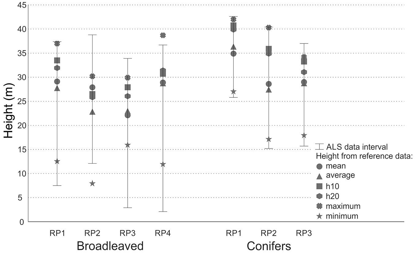
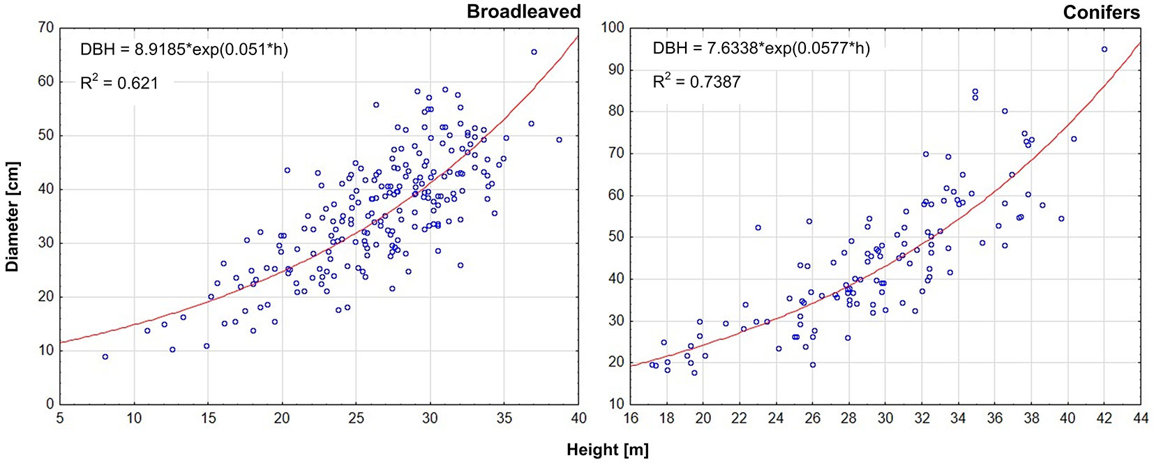
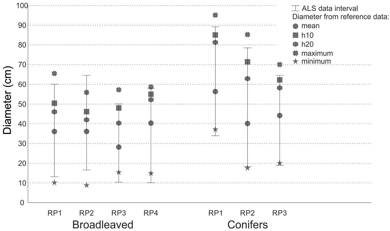
Fig. 3 shows the equations used to predict the tree diameter using ALS-derived individual height. Comparing the diameters obtained using ALS data with the diameters from reference data (Tab. 5), a trend similar to that observed for height estimation was observed. Indeed, errors in diameter estimation increased from the highest to the lowest spatial resolutions. Considering the parameters d10% and d20% the trend was the opposite. In the case of conifers, ALS-derived diameter values obtained at resolutions giving the most accurate identification of the tree number, closely approximated the mean diameter obtained from reference data. In the case of broadleaved species, the results were contradictory, as ALS-derived diameter was close to d20% in RP1, RP2 and RP4, while it was closer to the mean diameter from reference data in RP3. As expected, errors in diameter estimation using ALS data were greater than those observed for the height determination. For the mean diameter (dw), 29% of errors were <10% of the reference mean and 32% of errors were >20%. For the diameter d20%, 36% of errors were <10% and 35% of errors were >20%. Regarding d10% the situation was different: only 11% of the errors were lower than 10% from the reference mean, and 60% were greater than 20%. The errors in the mean diameter ranged from -12.1 to 15.3% at a resolution of 0.5 m (-12.1 to 5.3% for conifers, up to 15.3% for broadleaves). In the case of d10% the diameter was underestimated by 7-41%. These results were similar for both conifers and broadleaves in RP1, while better results were obtained for broadleaves in RP2 and for conifers in RP3. In the case of d20% of broadleaved species, overestimation was detected only in RP3 at a spatial resolution of 2 m, and close estimates were obtained in RP2 at a spatial resolution of 1.5 m. In all other cases d20% was underestimated. The range of errors was between -33.3 to 3.4%. Better results were obtained for broadleaves, where the error range at the spatial resolution of 2 m was between -4.2 to 3.4%. In the case of conifers, errors ranged from -10.4 to 21% at the spatial resolution of 2 m. A comparison of the diameter ranges derived from ALS data with reference data is shown in Fig. 4. In the case of conifers, there was an underestimation of the diameter, and there were no ALS-derived diameter values close to the reference maximum diameter. In the case of broadleaves, the situation was different in each RP.
Fig. 3 - Regression analysis between height and diameter based on data from field measurement. The equations used for deriving the diameter of individual trees (DBH) using the ALS-derived tree height (h) are shown for conifer and broadleaved species.
Tab. 5 - Mean tree diameter (in cm) calculated from ALS data at different spatial resolutions (0.5 to 2.0 m) compared with tree diameter values obtained from reference data. (RP): research plot; (d10%): dominant diameter based on the thickest 10% of trees in the RP; (d20%): dominant diameter based on the thickest 20% of trees in the RP.
| Dataset | Variable (Resolution) | RP1 | RP2 | RP3 | RP4 | |||
|---|---|---|---|---|---|---|---|---|
| broadleaved | conifers | broadleaved | conifers | broadleaved | conifers | broadleaved | ||
| ALS data | Mean diameter (0.5 m) | 38.3 | 56.0 | 35.9 | 42.2 | 29.1 | 38.8 | 46.5 |
| Mean diameter (1.0 m) | 42.8 | 61.6 | 39.9 | 49.6 | 31.9 | 46.5 | 47.8 | |
| Mean diameter (1.5 m) | 44.2 | 62.4 | 42.0 | 51.6 | 35.9 | 48.3 | 49.0 | |
| Mean diameter (2.0 m) | 45.5 | 64.2 | 40.2 | 56.3 | 41.7 | 49.2 | 51.0 | |
| Reference data |
Mean diameter (dw) | 36.1 | 56.3 | 36.0 | 40.1 | 28.1 | 44.2 | 40.3 |
| Dominant diameter (d10%) | 50.4 | 85.0 | 46.2 | 71.4 | 47.9 | 62.2 | 55.1 | |
| Dominant diameter (d20%) | 46.0 | 81.2 | 42.0 | 62.9 | 40.3 | 58.2 | 52.1 | |
Fig. 4 - Tree diameters calculated from reference data and tree height derived from ALS data for spatial resolution from 0.5 to 2 m.
Discussion
The basic step in deriving stand characteristics from ALS-collected data is identifying the trees, counting their number and locating their position. In this study ALS data were processed using an automatic approach and a spatial resolution ranging from 0.5 to 2 m. Our results confirmed the conclusions of Mikita et al. ([16]) that the spatial resolution of the raster layers significantly influences the identification of trees as well as the estimation of tree and stand dendrometric characteristics. In this study, when using the highest spatial resolution (0.5 m), the number of trees was overestimated by several hundred percent. This is due to the fact that many local maxima are usually identified when the crown surface obtained from the 3D cloud is highly detailed. On the other hand, using a low spatial resolution involves a generalization or “smoothing” of the DSM, leading to underestimate the number of extant trees on the ground.
The accuracy of tree identification was strictly dependent on the spatial resolution used: 1.0 m was the best resolution in RP 2 and RP 3, whereas 1.5 m was best in RP 1 and RP 4. The highest accuracy in each RP was above 84%. Vauhkonen et al. ([32]) stated that the accuracy of tree identification in Scandinavia and Central Europe is more than 70%. In broadleaved stands, the identification accuracy is lower (50%-60%) due to the complex nature of stand canopy and structure. Jing et al. ([8]) achieved a tree identification accuracy of 83% in mixed stands and 66% in broadleaved stands. The detection ratio for the spatial resolutions giving the highest number of identified trees (1.0 and 1.5 m) was in the range 69-75%. These results are similar to those achieved by Kaartinen et al. ([10]) and Vauhkonen et al. ([32]) testing several algorithms, while Zawawi et al. ([35]) obtained an identification accuracy of 24-56%.
Regarding the tree detection ratio, Reitberger et al. ([23]) reported values ranging from 56-94%, while Sterenczak & Miscicki ([28]) achieved a detection ratio of almost 82% for spruce. Yu et al. ([34]) obtained the highest detection ratio of 96% (though with an average value of 69%), and Khosravipour et al. ([11]) reported a mean value of 82%.
The vertical structure of the stand also affects tree identification using ALS-derived data. In this study, we considered only dominant trees with the crown in the upper canopy layer, as the identification of trees in the understorey layers using ALS-data is often difficult. Previous studies reported a percentage of trees identified in the understorey varying from 3-21% ([23]) to 40-45% ([21], [5]). On the other hand, Strîmbu & Strîmbu ([29]) stated that 95% of the trees in the understorey layer were identified in their study.
Tree height derived from ALS data is expected be underestimated since the laser impulses do not always reflect from the highest point of the canopy ([5], [33]). On the other hand, several studies reported an overestimation of tree height using ALS data. For example, Farid et al. ([4]) mentioned an overestimation of 77% when determining the tree height of young cottonwood (Populus fremontii S. Wats.) and mesquite (Prosopis velutina Wooton). The authors assume that the overestimation was caused by the reflection of laser impulses from higher trees located close to each other. Heurich ([5]) achieved a mean deviation between the height derived from ALS data and ground measurements of -0.54 m. Wezyk et al. ([33]) obtained slightly better results, from -0.12 to -0.9 m.
Kaartinen & Hyyppä ([9]) compared several methods from various countries, obtaining a tree height deviation in the range from -1.53 to 3.88 m. Similar results can be found also in Kaartinen et al. ([10]), where the models compared in the study of Kaartinen & Hyyppä ([9]) were extended. In the same study, it is mentioned that the best models achieved a RMSE of 0.6-0.8 m. Zawawi et al. ([35]) stated that the lowest estimated value of tree height from ALS data was 5.5 ± 1.5m. Mikita et al. ([16]) achieved a RMSE of 1.4-1.6 m, after excluding the trees in the understorey layer, while Latifi et al. ([12]) achieved a relative RMSE of 5.5%. In this study, the mean height derived from the ALS data (using the spatial resolution that resulted in the most accurate identification of trees, 1 m and 1.5 m) had an average deviation from reference data of 8.7%. The average differences were lower for h20% (5.9%) and higher for h10% (9.7%). Our results showed a lower precision when compared with those obtained by the aforementioned authors, though they are within the range indicated by Kaartinen & Hyyppä ([9]) and Kaartinen et al. ([10]). Further, we found that the differences in the identified height among different spatial resolutions ranged from 0 to 36%. The smallest differences in mean height were obtained using higher resolutions, and using lower resolutions in the case of h10% and h20%.
Tree height can be straightly obtained from the ALS data. On the contrary, the diameter has to be derived using existing relationships between tree height and diameter ([5], [2]). According to Persson et al. ([20]), it is possible to achieve an estimation of the diameter from ALS data with a difference of 10%. Latifi et al. ([12]) achieved a relative RMSE of 7.2% and a bias of -0.1% when estimating tree diameter from ALS data. Yu et al. ([34]) reported a RMSE of 10.32% for two coniferous wood species (Picea abies Karst. and Pinus sylvestris L.), while Järnstedt et al. ([7]) obtained a worse RMSE (25.3%) for the same tree species using a denser point cloud. In the present study, the diameter was derived from the regression models obtained using reference data collected in the individual plots. The mean diameter derived from ALS data (at the spatial resolution giving the most accurate tree identification - 1 and 1.5 m) was overestimated by 15.8%, on average, while d20% and d10% where underestimated by 14.1% and 21.7%, respectively. The difference in the mean diameter using a resolution of 0.5 m ranged from -8.7 to 10.7%. In general, however, the average difference of diameters is higher than the 10% mentioned by Persson et al. ([20]). Absolute differences in the derived diameters across all spatial resolutions range from 0 to 48%. As already mentioned, the smallest differences was detected using higher spatial resolutions for the mean diameter and lower resolutions for d10% and d20%.
Conclusions
Airborne laser scanning (ALS) is being more and more applied in forestry for tree detection and measurement. However, spatial resolution of ALS data can deeply affect the estimates of tree and stand characteristics. Using low spatial resolutions (0.5 m) we found that the number of trees in the stands is largely overestimated, while the opposite holds for high spatial resolutions (2.0 m). At intermediate resolutions of ALS data (1.0 m, 1.5 m) tree identification accuracy was over 84%.
The expectation that the most suitable spatial resolution for tree identification would be also the best for determining their height was not fulfilled. Compared with reference data (field measurements), ALS-derived mean height at resolution 0.5 m showed a deviation ranging from -3.1% to 10.4%. Optimal resolution for h10% and h20% estimation in conifers was 2.0 m, while contradictory results were obtained for broadleaved species. ALS-derived tree diameters were inferred using the regression analysis based on reference data. A spatial resolution of 0.5 m was the most suitable for determining mean tree diameter, with errors ranging from -8.7 to 10.7%. However, this method is not suitable for estimating d10% and d20%, as revealed by the large deviations found (sometimes >20%).
In this study, we applied an automatic approach for tree identification and estimation of tree dendrometric characteristics, which requires minimum interventions of the operator. Our results demonstrate that this approach is feasible and leads to mean tree height and diameter estimates which are consistent with similar studies. The main disadvantage is the need of a more generalized model for the relationships between tree diameter and height to be used for ALS-derived diameter estimation. Further analyses of larger datasets are needed to further test the feasibility of the adopted approach for the detection of tree dendrometric characteristics from ALS data.
Acknowledgements
This research was supported by the projects: Centre of Excellence “Decision support in forest and country”, ITMS: 26220 120069, supported by the Research and Development Operational Programme funded by the ERDF (50%); and by the Slovak Research and Development Agency, project APVV-15-0393 “Innovations in the forest inventories based on progressive technologies of remote sensing” (50%).
References
Gscholar
Gscholar
Gscholar
CrossRef | Gscholar
CrossRef | Gscholar
Gscholar
Online | Gscholar
Gscholar
Gscholar
Online | Gscholar
Gscholar
Gscholar
Online | Gscholar
CrossRef | Gscholar
Online | Gscholar
Gscholar
Gscholar
Authors’ Info
Authors’ Affiliation
Martina Levická
Ján Tuček
Department of Forest Management and Geodesy, Technical University in Zvolen, T. G. Masaryka 24, 960 53 Zvolen (Slovakia)
Soil Science and Conservation Research Institute, Gagarinova 10, 827 13 Bratislava (Slovakia)
Department of Forest Policy, Economics and Forest Management, National Forest Centre
The Institute of Foreign Languages, Technical University in Zvolen, T. G. Masaryka 24, 960 53 Zvolen (Slovakia)
Corresponding author
Paper Info
Citation
Smreček R, Michnová Z, Sačkov I, Danihelová Z, Levická M, Tuček J (2018). Determining basic forest stand characteristics using airborne laser scanning in mixed forest stands of Central Europe. iForest 11: 181-188. - doi: 10.3832/ifor2520-010
Academic Editor
Agostino Ferrara
Paper history
Received: Jun 13, 2017
Accepted: Dec 13, 2017
First online: Feb 19, 2018
Publication Date: Feb 28, 2018
Publication Time: 2.27 months
Copyright Information
© SISEF - The Italian Society of Silviculture and Forest Ecology 2018
Open Access
This article is distributed under the terms of the Creative Commons Attribution-Non Commercial 4.0 International (https://creativecommons.org/licenses/by-nc/4.0/), which permits unrestricted use, distribution, and reproduction in any medium, provided you give appropriate credit to the original author(s) and the source, provide a link to the Creative Commons license, and indicate if changes were made.

Web Metrics
Breakdown by View Type
Article Usage
Total Article Views: 48668
(from publication date up to now)
Breakdown by View Type
HTML Page Views: 40446
Abstract Page Views: 3144
PDF Downloads: 3824
Citation/Reference Downloads: 27
XML Downloads: 1227
Web Metrics
Days since publication: 3056
Overall contacts: 48668
Avg. contacts per week: 111.48
Article Citations
Article citations are based on data periodically collected from the Clarivate Web of Science web site
(last update: Mar 2025)
Total number of cites (since 2018): 5
Average cites per year: 0.63
Publication Metrics
by Dimensions ©
Articles citing this article
List of the papers citing this article based on CrossRef Cited-by.
Related Contents
iForest Similar Articles
Research Articles
Three-dimensional forest stand height map production utilizing airborne laser scanning dense point clouds and precise quality evaluation
vol. 10, pp. 491-497 (online: 12 April 2017)
Technical Advances
Forest stand height determination from low point density airborne laser scanning data in Roznava Forest enterprise zone (Slovakia)
vol. 6, pp. 48-54 (online: 21 January 2013)
Research Articles
Integrating area-based and individual tree detection approaches for estimating tree volume in plantation inventory using aerial image and airborne laser scanning data
vol. 10, pp. 296-302 (online: 15 December 2016)
Review Papers
Accuracy of determining specific parameters of the urban forest using remote sensing
vol. 12, pp. 498-510 (online: 02 December 2019)
Research Articles
Integration of tree allometry rules to treetops detection and tree crowns delineation using airborne lidar data
vol. 10, pp. 459-467 (online: 04 April 2017)
Research Articles
Are we ready for a National Forest Information System? State of the art of forest maps and airborne laser scanning data availability in Italy
vol. 14, pp. 144-154 (online: 23 March 2021)
Technical Reports
Remote sensing of american maple in alluvial forests: a case study in an island complex of the Loire valley (France)
vol. 13, pp. 409-416 (online: 16 September 2020)
Research Articles
Prediction of stem diameter and biomass at individual tree crown level with advanced machine learning techniques
vol. 12, pp. 323-329 (online: 14 June 2019)
Research Articles
Comparing image-based point clouds and airborne laser scanning data for estimating forest heights
vol. 10, pp. 273-280 (online: 23 February 2017)
Review Papers
Remote sensing-supported vegetation parameters for regional climate models: a brief review
vol. 3, pp. 98-101 (online: 15 July 2010)
iForest Database Search
Search By Author
Search By Keyword
Google Scholar Search
Citing Articles
Search By Author
Search By Keywords
PubMed Search
Search By Author
Search By Keyword


