Remote sensing of american maple in alluvial forests: a case study in an island complex of the Loire valley (France)
iForest - Biogeosciences and Forestry, Volume 13, Issue 5, Pages 409-416 (2020)
doi: https://doi.org/10.3832/ifor3237-013
Published: Sep 16, 2020 - Copyright © 2020 SISEF
Technical Reports
Abstract
Due to their particular topographic position between land and river, riparian forests are ecosystems rich in biodiversity. In France, along the Middle Loire (from Nevers to Angers), Black poplar (Populus nigra L.) forests are often in mixtures with the American maple (Acer negundo L.), introduced into the country in the 18th century. We tested the detectability of American maple by LiDAR and very high-resolution multispectral imagery on an island complex. We found that coupling the point cloud height standard deviation with a vegetation index in the red, green and blue spectrums discriminated American maple with a success rate of more than 90%.
Keywords
Acer negundo, American Maple, Box Elder, Populus nigra, Black Poplar, Airborne Laser Scanning, Remote Sensing, Exogenous Woody Species, Loire River
Introduction
Riparian forests are a key component of river ecosystems due to their position at the interface between water and land ([28], [13]). In the anabranch river landscape of the Middle Loire in France (around 400 km between Nevers and Angers), alluvial forests represent a significant part of the vegetation biomass ([12]). Because of their vulnerability to anthropomorphic impact ([31]), riparian forests are considered to be habitats of Special Community Interest in the Habitats Directive 92/43/CEE (EUNIS: G1.11 - [4]). In these habitats, groundwater reduction due to channel digging ([11]), water pollution and the introduction of exogenous woody species have perturbed the natural colonization by Salicaceae of river banks and islands ([1]). For example, the American maple (Acer negundo L., AC) was introduced in France in 1732 ([10]) and is now commonly found in native Black poplar (Populus nigra L., PN) stands ([3]). In addition, the reintroduction of the European beaver in the 1970’s indirectly favored colonization by the introduced species since beaver consumes the Black poplar but not the American maple.
In view of the above-mentioned elements, regular monitoring of riparian forests is important for their conservation and management, all the more so in a context of global warming, as these forests vary with the water level from one year to another and present multiple aspects. Thus, mapping these alluvial forests and updating the maps on a near-annual basis are the most appropriate tools to ensure quality monitoring. Currently, cartography has made tremendous progress thanks to Geographic Information Systems (GIS) software and satellite or aerial imagery ([9], [17]). In France, the National Forest Inventory carries out a permanent inventory of forest resources and provides a great deal of data, including interactive maps. Data are collected at both the stand and tree levels. At the stand level, the forest cover type is interpreted from infrared aerial images at a 50-cm resolution. The final product is a vector layer (BD Foret V2) with polygons of 0.5 ha minimum attributed to 32 categories of species composition. However, neither AC nor PN has a category of its own, so this data cannot be used to monitor their spatial dynamics. At the tree level, many parameters are recorded on the NFI sample plots in different scientific domains such as dendrometry, botany and pedology ([15]). Tree data include diameter, species and position, and height for a sub sample. However, precise plot locations are not publicly available, which prevents cross-analysis with external geographical data. Furthermore, plot density is 1 plot/2km2 with surveys only every 5 years, thus making the data unsuitable for statistical analysis of small areas.
Aerial imagery provides only two-dimensional images that do not enable direct measurement of the vertical components of the forest canopy. However, in the beginning of the twenty-first century, technological advances in drones and active remote sensing, in particular through the development of new sensors, opened promising perspectives for accessing forest structures ([5]). For instance, UAVs (Unmanned Aerial Vehicles) with Light Detection and Ranging (LiDAR) provide a three-dimensional geo-referenced point cloud corresponding to the surface objects that intercept the laser pulses from a scanner mounted on an aircraft ([2]). Though the first uses of LiDAR were mainly devoted to digital terrain models ([34]), numerous applications in forestry have since been investigated.
An overview of the bibliography reveals that there are two main approaches to tree crown delineation from LiDAR data. The first one aims to model tree shape directly in the LiDAR cloud, but this process is quite complex ([26], [18]). The second approach involves reducing the LiDAR cloud from 3D to 2D. This simplification is interesting because rasters have a longer development history than other approaches ([25], [35]). The 3D-to-2D approach relies on the detection of treetops in the canopy height model (CHM). Then, the crowns are delineated with the watershed algorithm, which reverses the image and considers the crown envelope as a basin ([23], [20]).
To ensure proper delineation of the trees, the algorithm’s parameters must be carefully chosen in order to correspond to tree allometries, which are often species- and structure-specific. Applying watershed theory to the forest requires some intrinsic parameters for tree architecture, such as the distance to the nearest treetop, crown size, etc.
Our main goal was to test the ability of the various parameters in the tree segmentation function of the “lidaRtRee” package ([27]) running on free R software to predict American maple stands in Black poplar island forests. Another objective of this technical paper is to assess the ability of combined LiDAR data and multispectral data acquired by unmanned aerial vehicles (UAVs) to distinguish American maple from Black poplar at the tree level. The test site was located in a French National Nature Reserve along the Loire River. We focused on the use of open-source software tools with visual interpretation for training and validation steps to ensure that the method could be applied to larger areas.
Material and methods
Study area
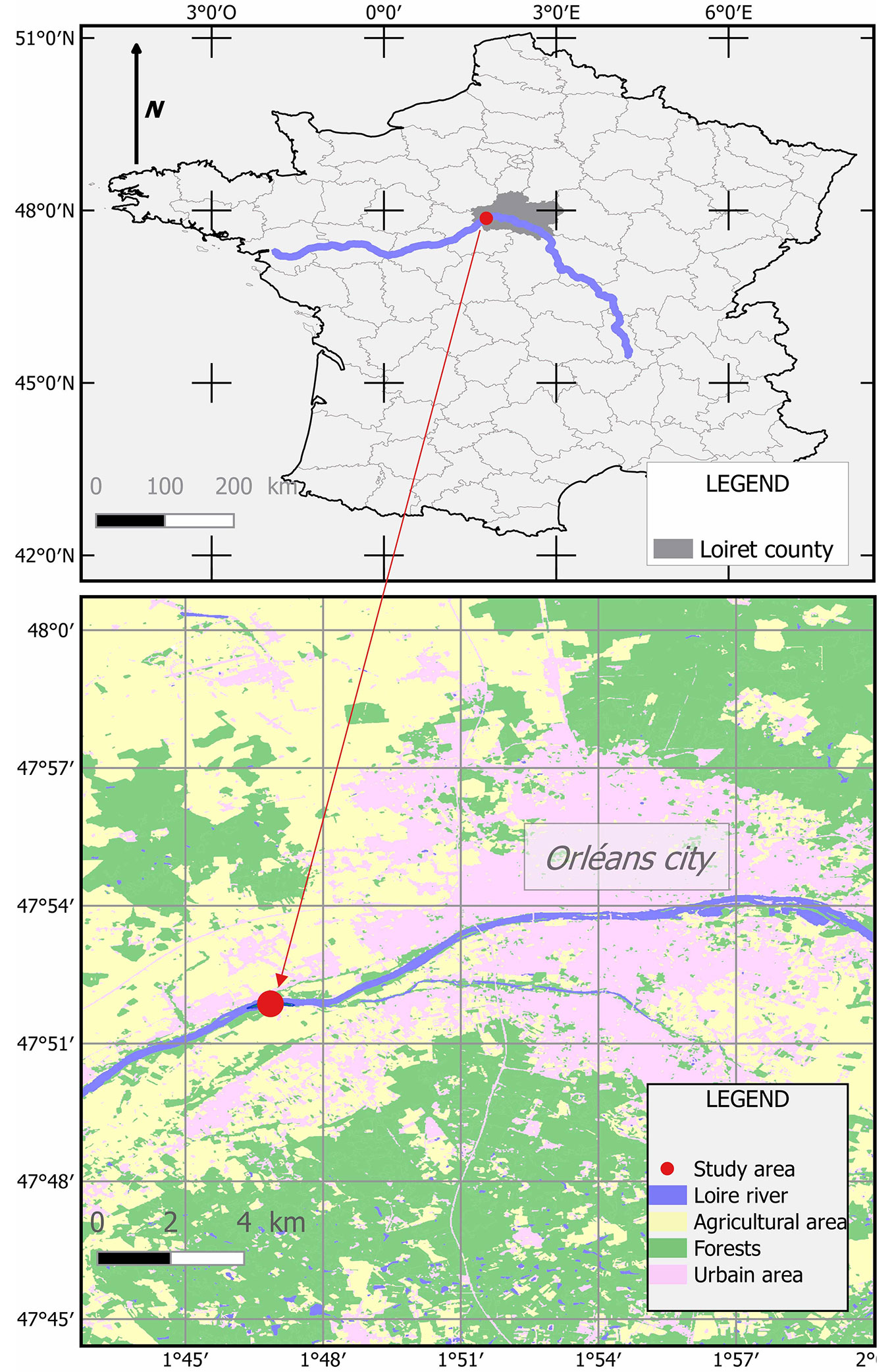
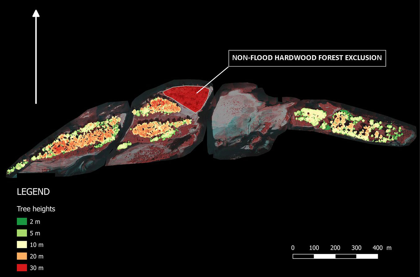
The research was conducted in central France in the Loiret county, on the Mareau-aux-Prés islands in the Loire River (within the boundaries of the Saint-Mesmin National Nature Reserve) near the village of Mareau-aux-Prés (Fig. 1), approximately 10 km downstream from the city of Orléans (47° 51′ 51.88″ N, 01° 46′ 52.84″ E). The total area of the experiment was about 10 ha and elevation ranged from 84 to 89 m a.s.l. The mosaic of four islands (Fig. 2) is mainly dominated by species from the Salicaceae family - adult black poplar and willow shrubs (Salix spp.) - except for the central island (C) where, in September 2012, the vegetation was uprooted and the island was leveled and lowered in order to maintain the flow capacity of the Loire river and to prevent floods. A new sedimentary bar appeared in spring 2013 and was colonized by Black poplar and willow seedlings; this island was therefore surveyed with the three other islands.
Fig. 1 - Study area. The Mareau-aux-prés islands are located within the large National Natural Reserve of Saint-Mesmin, downstream from Orléans (Loiret, France).
Image and LiDAR acquisition
Because terns were nesting on the banks, we were allowed to fly over the islands only after August 15. The UAV flights were carried out on 20 and 21 August 2017 by “L’Avion Jaune”, a French aerial mapping operator using an octorotor FOX-C8 Onyxstar®. The level of the Loire River was one meter above zero, corresponding to summer low water. Eight successive flights occurred; three with a LiDAR sensor, then five others with a camera. LiDAR data were acquired by a YellowScan Surveyor® (YellowScan, Montferrier-sur-Lez, France), which included an onboard computer controlling three main components: a Velodyne laser scanner (VLP16), a Global Navigation Satellite System (GNSS) and an Inertial Navigation System (INS) built by Applanix (APX15). The flight height for the LiDAR was 45 m with a line spacing of 45 m and a sidelap of 60%. The average point density per m2 was 215. Multispectral imagery was acquired with a mapping system conceived by L’Avion Jaune. The latter consisted of a pair of identical digital single-lens reflex cameras (Canon® EOS 500D) - one modified to assess the near infrared (NIR) wavelength, while the other unmodified camera assessed the visible wavelengths (RGB). The flight height for multispectral acquisition was 100 m with a sidelap of 60% and a frontlap of 80%.
Workflow
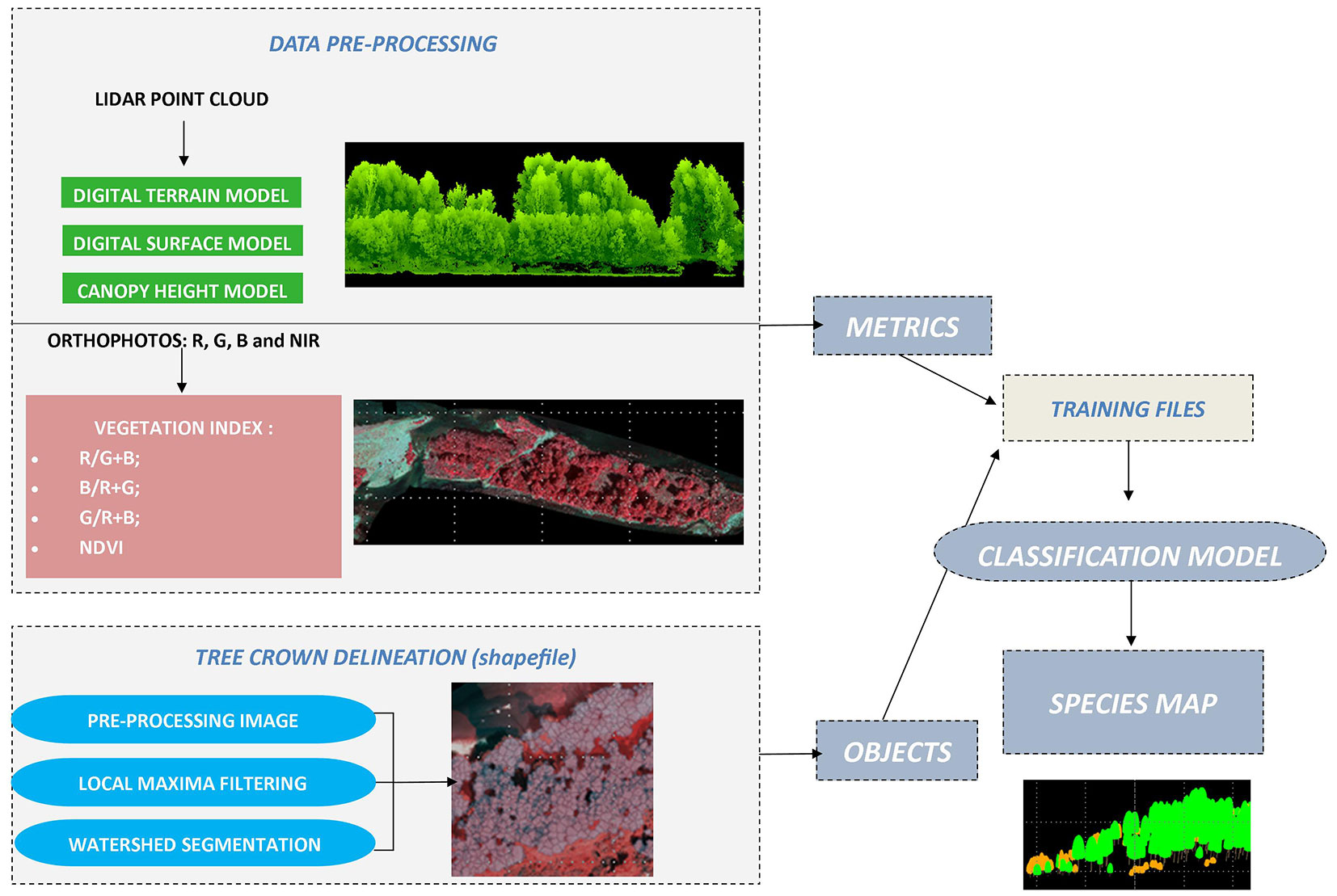
The workflow was divided into three main steps (Fig. 3): (i) data pre-processing; (ii) tree crown delineation; (iii) model classification.
Data pre-processing: LiDAR data
Raw data processing was done by the mapping operator. LiDAR data were processed by successively running them through the PosPAC software by Applanix, a Surveyor QGIS plugin by YellowScan, and TerraMatch and TerraScan modules by TerraSolid. The classified point cloud was delivered in LAS format. The Digital Terrain Model (DTM) and the Canopy Height Model (CHM) were delivered in Geotif format at 0.2-m resolution. In order to compare different tree segmentations, we created a flood and non-flood forest mask within the mosaic of islands (Fig. 4.). Since American maple mainly colonizes river banks ([13]), we excluded the hardwood forest (oak, elm, ash), located on higher terrain (in the non-flood area on island B), and retained only values between 0 and 2.5 m in height. This general mask was applied to all image treatments, including point clouds, DTM and CHM files, and orthophotos.
Data pre-processing: multispectral imagery and vegetation index
Multispectral imagery processing was performed according to scripts developed by L’Avion Jaune and the Correlator3D software by Simactive. An orthophoto with four spectral bands (blue, green, red and near-infrared) was generated with a Ground Sample Distance (GSD) of 0.02 m. The orthophoto was resampled to 0.2 m for consistency with the CHM.
Then four simple vegetation indices, excluding the infrared wavelength, were computed: (i) Red / (Green + Blue); (ii) Green / (Red + Blue); (iii) Blue / (Green + Red). We also computed the (iv) Normalized Difference Vegetation Index (NDVI - [32]).
Tree crown delineation
This step is important because it determines the location and extent of the crowns. Subsequently, the data extracted inside the delineated crowns are used to select the discrimination variables in the classification step. Tree segmentation was performed with the “treeSegmentation” function from the “lidaRtRee” package ([27]) of the R software ([30]). Delineation was based on a 3-phase approach, with each phase requiring several values for parametrization.
First, we applied filters to remove noise from the CHM file. A “salt-and-pepper” noise generally appears when there are CHM pixels with no corresponding laser points (due to the shading effect of trees, for example), or when there is a low number of pixels inside the canopy. The low and zero values were removed by applying a closing filter on a 3-pixel-wide neighborhood, which is the default parameter. We next applied a Gaussian filter to smooth out small local variations; this prevents multiple branches from being detected as separate apices ([26]). Smoothing intensity is driven by the sigma value of the Gaussian filter, which must be adapted to the tree structure and species. In our study, we tested all values from 0.1 to 0.9.
The second step was to select maximum tree height. We first set a minimum treetop height parameter with a value of 3 m in order to avoid confusion with local maxima related to herbs and shrubs. For example, in summer 2017, nettles (Urtica sp.) reached as much as 2.5 m in height. We then used horizontal neighborhood parameters to take into account the minimum distance between one maximum treetop height and nearby crowns of the same height. Considering the important overlap between crowns in the forest, no selection based on minimum distance was applied (i.e., a minimum distance of zero was applied).
The third step was tree crown delineation. To segment the crown extension, we applied a marked-based watershed algorithm. Segments in watershed analysis are delineated by selecting local maxima as the start points of watersheds created by flooding a model surface; this process reverses the CHM. Each local maximum has its corresponding crown (segment). In order to exclude neighboring shrubs from the crown segment, two operations were performed: (i) pixels lower than 3 m were excluded from the crowns; (ii) inside each crown, we further excluded the pixels lower than the crown proportion multiplied by treetop height. The resulting parameter reflects the ratio between crown depth and tree height, and must be adapted depending on stand structure. We tested all values between 0.1 (the tree crown extended almost to the ground) and 0.9 (the crown was located within the highest 10% of the tree).
The different parameters tested and their values are listed in Tab. 1.
Tab. 1 - Parameters of the “treeSegmentation” function (“lidaRtRee” package). (*): Variables tested and their range of values.
| Name | Function |
|---|---|
| nFilter, nlSize | Prevents “salt and pepper” where no laser points are recorded. We used the default option “Closing” and 3 for size. |
| sigma * | Prevents branches in a crown from being considered as trees. We tested from 0.1 to 0.9 |
| dmin/dprop | Treetop minimum distance to the next higher pixel and distance as a proportion of height to the next higher pixel. We set these two values at “0” due to crown overlap |
| hmin | Minimum treetop height: 3 m due to tall nettles |
| crownProp * | Minimum height of tree crown as a proportion of treetop height. We tested from 0.1 to 0.9 |
| crownMinH | Minimum crown height. We set this value at 3 m. |
Classification model: reference data
In order to build a model capable of separating Acer negundo (AC) and Populus nigra (PN), a reference dataset was created by using the 0.02 cm resolution orthophotos. Very high resolution imagery, such as provided by UAV, are ideal for photointerpretation ([17]). The operator selected a total of 316 disks of 1 m diameter and classified them as AC (157) or PN (159). Although the operator is both a botanist and an experienced GIS operator with exhaustive field knowledge of the study site, classification errors might be present in this reference dataset.
Classification model: variables tested
In order to classify the two tree species, variables were computed for each delineated crown based on the CHM, the point cloud and the orthophoto intersecting the crown segments. Tab. 2 presents the variables tested sorted by category: tree metrics (T), LiDAR metrics (L) and orthophoto indices (O). We tested different combinations: (i) T + L + O; (ii) T + L; (iii) L + O; (iv) T + O; (v) T; (vi) L; (vii) O. This made seven possible combinations mixed with nine possibilities for the Gaussian filter and nine possibilities for the crown proportion (567 processes).
Tab. 2 - Metrics computed.
| Metrics group | Metrics | Description |
|---|---|---|
| Tree metrics (T) | s | Crown surface |
| v | Crown volume | |
| chm.sd | Height standard deviation | |
| zskew | Skewness of height distribution | |
| zkurt | Kurtosis of height distribution | |
| zentropy | Normalized Shannon diversity index of height distribution | |
| LiDAR metrics (L) | zpcum1 | Cumulative percentage of return in the 1st layer |
| zpcum2 | Cumulative percentage of return in the 2nd layer | |
| zpcum3 | Cumulative percentage of return in the 3rd layer | |
| zpcum4 | Cumulative percentage of return in the 4th layer | |
| zpcum5 | Cumulative percentage of return in the 5th layer | |
| zpcum6 | Cumulative percentage of return in the 6th layer | |
| zpcum7 | Cumulative percentage of return in the 7th layer | |
| zpcum8 | Cumulative percentage of return in the 8th layer | |
| zpcum9 | Cumulative percentage of return in the 9th layer | |
| isd | Standard deviation of intensity | |
| iskew | Skewness of intensity distribution | |
| ikurt | Kurtosis of intensity distribution | |
| ipcumzq10 | Percentage of intensity returned below the 10th percentile of height | |
| ipcumzq30 | Percentage of intensity returned below the 30th percentile of height | |
| ipcumzq50 | Percentage of intensity returned below the 50th percentile of height | |
| ipcumzq70 | Percentage of intensity returned below the 70th percentile of height | |
| ipcumzq90 | Percentage of intensity returned below the 90th percentile of height | |
| Orthophoto Indices (O) | m.r.gb | Median (R/(G+B)) |
| m.g.rb | Median (B/(R+G)) | |
| m.b.rg | Median (B/(R+G)) | |
| m.ndvi | Median (NDVI) | |
| sd.r.gb | Standard deviation of (R/(G+B)) | |
| sd.g.rb | Standard deviation of (B/(R+G)) | |
| sd.b.rg | Standard deviation of (B/(R+G)) | |
| sd.ndvi | Standard deviation of (NDVI) |
Direct height variables such as CHM, DTM and point cloud minimum, mean or maximum values were a priori discarded from the analysis, based on our knowledge of fluvial dynamics. Indeed, local island topography changes annually due to sand accretion and erosion. Therefore, keeping a fixed height topography value set on the Mareau-aux-Prés complex would have falsified our extrapolation for the Middle-Loire stretch of the river. Secondly, due to the propagation strategy of the American maple, whose seeds arrive by cohort on exposed river banks ([33]), a classification based on height values might have merely reflected the age difference between PN and AC, particularly at our study location in the National Reserve. This would also have led to erroneous extrapolated results for other areas along the Loire River.
Classification model: decision tree
In order to select discriminating variables, we used Decision Tree in the R party package ([16]). To confirm our results, we ran each decision tree 250 times.
Results
The entire classification process was run on the riparian forests of the Mareau-aux-Prés islands (Islands: A, B and D - Fig. 4), excluding the hardwood forests. We tested 567 processes and report their overall accuracy and standard deviation in Tab. S1 (Supplementary material).
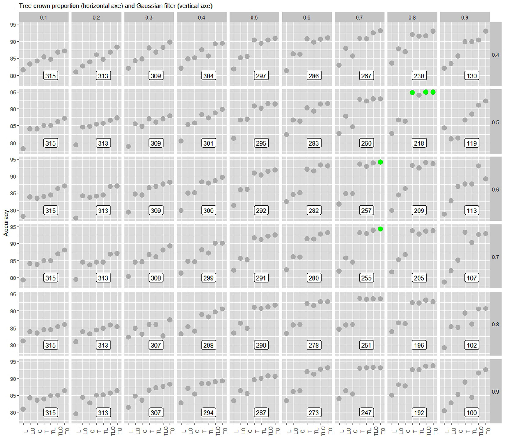
The accuracy of our classification varied with Gaussian filter and with crown proportion according to metrics group. In Fig. 5, we only present the results from Gaussian filter 0.4 because below this threshold, none of the models succeeded (see Tab. S1 in Supplementary material). Best overall accuracy is represented by green dots for a value greater than 94%. These results concerned all of the metrics groups since the best combinations were: T, TLO, and TO with crown proportions from 0.7 to 0.8 and Gaussian filters from 0.5 to 0.7. To select the best metrics groups, we had to take into account the number of trees used for training/validation. Indeed, as shown in Fig. 5, we observed that the more the crown proportion and the Gaussian filter increased, the more the number of trees decreased. We then found the best compromise between the best precision and the largest number of trees for training/validation (out of a total of 316 trees selected by visual interpretation). Tab. 3 shows the results of the green dot values and their standard deviations in Fig. 5. We observed that overall accuracy and standard deviations were close and that the number of trees used for training/validation was actually relevant. Finally, we opted for Gaussian filter values of 0.7 and 0.6, and for a crown proportion value of 0.7.
Fig. 5 - Overall accuracy (% on the y-axis) of the metrics groups tested (on the x-axis) according to crown proportion (values in gray horizontal) and Gaussian filter (values in gray vertical). Metrics groups tested were: Tree metrics (T), LiDAR metrics (L) and Orthophotos indices (O). Combinations tested were: T+L+O, T+L, L+O, T+O, T, L, O. White rectangles correspond to the number of trees used for training and validation. Green dots correspond to an accuracy > 94%.
Tab. 3 - Overall accuracy assessment (mean ± standard deviation of 250 repetitions) and number of trees in the reference dataset for the metrics groups selected according to the tree segmentation parameters. (T/V): training / validation; (T): tree metrics; (L): LiDAR metrics; (O): Ortophotos indices.
| Gaussian filter | crownProp | T/V tree number | TLO | TO | T |
|---|---|---|---|---|---|
| 0.7 | 0.7 | 255 | - | 94.3 ± 2.7 | - |
| 0.6 | 0.7 | 257 | - | 94.1 ± 2.5 | - |
| 0.5 | 0.8 | 219 | 94.8 ± 2.5 | 94.8 ± 2.4 | 94.7 ± 2.3 |
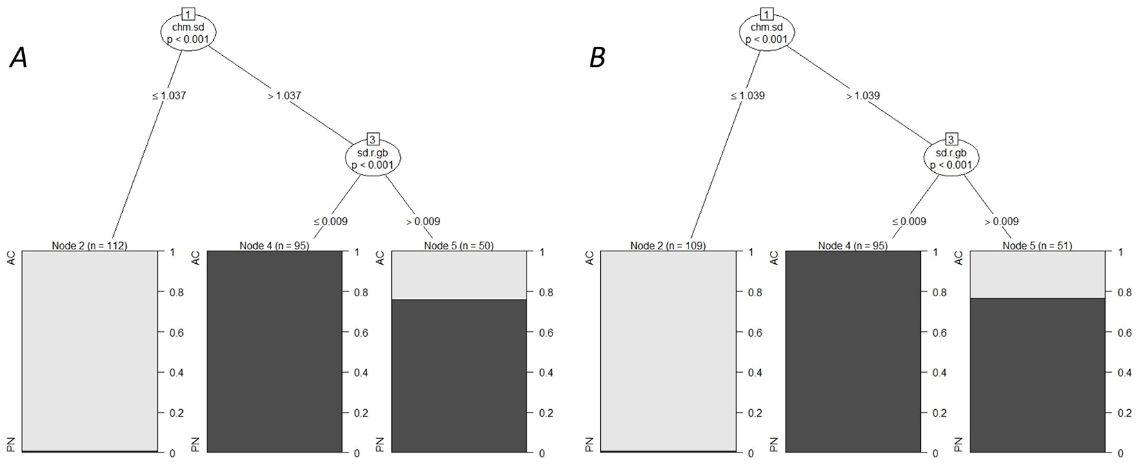
Fig. 6 shows that, for both values of Gaussian filter (A and B), point cloud height standard deviation was the most robust discriminating variable to distinguish AC from PN. Indeed, even below a height value of just one meter, we consistently detected AC. Above this threshold, a vegetation index Red / (Green + Blue) standard deviation below 0.009 discriminated PN. However, above 0.009 there was an uncertainty of more than 20% for the prediction of PN.
Fig. 6 - Conditional inference tree for the tree species data: AC in light gray, PN in dark gray. (A) Gaussian filter = 0.6, Crown proportion = 0.7, number of trees for training/validation = 257. (B) Gaussian filter = 0.7, Crown proportion = 0.7, number of trees for training/validation = 255. For each inner node, the Bonferroni-adjusted p-values are given; the fraction of tree species is displayed for each terminal node.
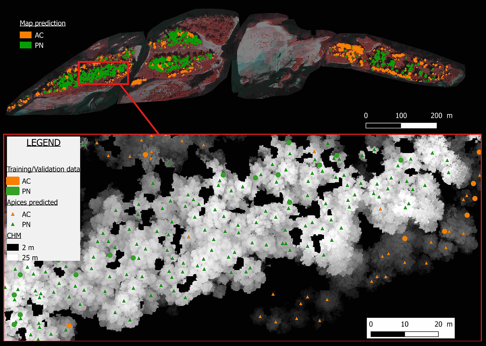
Fig. 7 presents a prediction map showing that American maple is mainly confined to the outer edges of the islands.
Fig. 7 - Prediction map. Upper part of the figure: prediction map of the American maple (AC, in orange) and Black poplar (PN, in green). Lower part of the figure: an example on a part of the furthest island from the study: circles represent the data interpreted visually, triangles represent the predicted apices, symbology of colors is identical to that previously described.
Discussion
Our results show that, within the National Nature Reserve of Mareau-aux-Prés, point cloud height standard deviation and the standard vegetation index Red / (Green + Blue) predict the presence of American maple (Acer negundo L.) in more than 90% of the riparian Black poplar (Populus nigra L.) forests.
The retained variables correspond respectively to the groups of tree metrics (point cloud height standard deviation) and the orthophoto indices (standard vegetation index).
In the context of introduced species in alluvial forest contexts, our results reinforce the use of LiDAR coupled with photogrammetry ([22], [17]), although comparison with previous research also displays differences. In a Mediterranean riparian forest, Dunford et al. ([11]) distinguished five classes including four tree species with an overall accuracy of 91% from a single RGB image of 13 cm resolution obtained from UAV. Their reference data consisted of homogeneous terrain units identified on the field with an inclusive sampling and then digitized on the imagery. The overall accuracy dropped to 71% at the mosaic scale, partly because of radiometry differences in images. The greater accuracy achieved in our case might be explained by the height information added by LiDAR data, as well as the lower number of classes. The radiometry issue might be a problem when analysing larger areas which would require more images and acquisition time with a UAV. With bi-spectral LiDAR data, Laslier et al. ([19]) classified eight species of a riparian forest in Normandy (France) with an overall accuracy of 67%. Their study also highlights the importance of elevation metrics for classification. Intensity-related metrics did not bring much improvement in their classification, suggesting that spectral information of LiDAR might not be as straigthforward to use as with imagery. Differences with our results might be explained in part by the fact that they explored a larger gradient of tree species, while we limited ourselves to two species. A wider variety of species can present complex internal canopy structures revealed by LiDAR metrics. When comparing the importance of variables from multispectral and hyperspectral imagery and full-wave form LiDAR for the classification of four tree species in a temperate forest, Heinzel & Koch ([14]) found out that the NIR channel had great importance. Height metrics derived from LiDAR were not selected, but there was one LiDAR metric linked with the internal structure. Differences with our findings might be due to the fact that they considered both deciduous and coniferous species, which have different reflectance in NIR. Dalponte et al. ([6]) showed that LiDAR height metrics improved the classification of mountainous forests into seven tree species compared to multispectral data only. The variability in findings available in the literature shows that depending on species and forest structures, and probably on acquisition period, there are variations in the importance of metrics of different types for species classification.
The results obtained here are rather encouraging regarding the potential for mapping AN dynamics on larger areas with simple variables. Meanwhile, we must be aware of limitations as pointed out by Huylenbroeck et al. ([17]) regarding upscaling of results. In the case of longer stretch of river, the relevance of spectral indices might decrease because of issues with radiometric calibration of images and greater variability of forest species, structure and phenology. The use of reference data based only on photointerpretation might also introduce bias or error in the training and validation processes, but it makes also possible to build larger datasets by taking advantage of very high resolution imagery available from UAV. It is clear that this step is highly dependent both on the operator’s experience in visual interpretation and his knowledge of the study area, but it is essential to calibrate the predictions as well as possible ([22], [8]). The trade-off between variability representation thanks to sample size and noise due to visual interpretation still has to be investigated in order to design cost-efficient operational protocols for the acquisition of reference data for species mapping in larger areas.
However, there are limitations to our findings, especially for Black poplar. Indeed, our results do not take into account an indirect beaver-consumption effect. By consuming Black poplar, the beaver generates holes in the canopy that allow the LiDAR to better penetrate the crowns at the tree scale. If we were to extend our work to all of the Middle-Loire from Nevers to Angers (a distance of about 400 km), the results would be at least partially dependent on beaver population density per linear kilometer. How accurate would our classification model be without the presence of the beaver?
One way to solve this problem would be to repeat overflights and test the crown delineation function with tree shape settings. This method was tested on Belgium riparian forests by Michez et al. ([24]). Although the image analyses differ according to our study accuracy is greatly increased by repeated overflights. More overflights would likely improve detectability for American maple under the canopy of the taller Black poplars.
Lastly, as Pirotti et al. ([29]) show in their study, we could also test other tree crown delineation algorithms such as “Li 2012” and “Dalponte 2016”. The Dalponte 2016 algorithm ([7]) is similar to the one we used in this study since it starts from rather similar parameters and then segments the CHM. On the other hand, Li’s 2012 algorithm ([21]) does not use a CHM and works directly on the point cloud instead. Though algorithms based directly on the point cloud seem to take more processing time, they could enable researchers to explore the canopy structure of these Loire-island forests.
Conclusion
American maple (Acer negundo L.) is an introduced species, which competes with the endemic Black poplar (Populus nigra L.). We used an airborne LiDAR scanner and imagery-derived vegetation index data to discriminate American maple from Black poplar with 90% accuracy on a complex of four islands inside the National Nature Reserve of Saint-Mesmin in the Loire River (France), based on a training and validation dataset obtained by photointerpretation. Mapping the American maple is all the more important since beavers (reintroduced in the 1970s) do not consume it, though it consumes Black poplar. We found that tree crown delineation is optimized by the “treeSegmentation” function from the “lidaRtRee” package ([27]) running under free R software ([30]). We tested two important parameters of this function: the Gaussian filter and crown proportion. The first parameter prevents big branches in a crown being considered as trees. The second optimizes the proportion of the crown relative to the total height. We found that the best values for the Gaussian filter and crown proportion were respectively 0.7 (and 0.6) and 0.7. We also found that the best predictors were point cloud height standard deviation and the standard deviation of a simple vegetation index based on RGB wavelengths, Red/ (Green + Blue).
Acknowledgements
This study is part of the BioMareau project, funded within the framework of the Loire River Interregional Program 2014-2020”. Funding institutions are the Centre-Val de Loire Region (no. 2016-00108348), INRA, IRSTEA and the European Union (Europe being engaged in the Loire basin through the EU operational program of the European Regional Development Fund, no. 2016-EX000604). The BioMareau project has been approved by the CNRS Loire LTER “Zone Atelier Loire” and the regional MIDI (Habitat and Diversity) research network. Michel Chantereau and Damien Hémeray from the National Natural Reserve of Saint-Mesmin are acknowledged for their interest and their support for science at the Mareau-aux-prés Islands.
We also thank Vicki Moore for her relevant editorial remarks.
References
Gscholar
CrossRef | Gscholar
Gscholar
CrossRef | Gscholar
Gscholar
Online | Gscholar
Online | Gscholar
Gscholar
Gscholar
Authors’ Info
Authors’ Affiliation
Richard Chevalier
INRAE Val de Loire, Site de Nogent-sur-Vernisson, Domaine des Barres 45290 Nogent-sur-Vernisson (France)
Univ. Grenoble Alpes, INRAE, UR LESSEM, F-38402 St-Martin-d’Hères (France)
L’AVION JAUNE, 1 chemin du Fescau, 34980 Montferrier-sur-Lez (France)
INRAE Val de Loire, UMR 0588 INRA-ONF BioForA, 2163 Av. de la Pomme de Pin, CS 40001 Ardon, 45075 Orléans Cedex 2 (France)
Corresponding author
Paper Info
Citation
Martin H, Monnet J-M, De Boisvilliers M, Chevalier R, Villar M (2020). Remote sensing of american maple in alluvial forests: a case study in an island complex of the Loire valley (France). iForest 13: 409-416. - doi: 10.3832/ifor3237-013
Academic Editor
Matteo Garbarino
Paper history
Received: Sep 13, 2019
Accepted: Jul 08, 2020
First online: Sep 16, 2020
Publication Date: Oct 31, 2020
Publication Time: 2.33 months
Copyright Information
© SISEF - The Italian Society of Silviculture and Forest Ecology 2020
Open Access
This article is distributed under the terms of the Creative Commons Attribution-Non Commercial 4.0 International (https://creativecommons.org/licenses/by-nc/4.0/), which permits unrestricted use, distribution, and reproduction in any medium, provided you give appropriate credit to the original author(s) and the source, provide a link to the Creative Commons license, and indicate if changes were made.
Web Metrics
Breakdown by View Type
Article Usage
Total Article Views: 40658
(from publication date up to now)
Breakdown by View Type
HTML Page Views: 33623
Abstract Page Views: 3235
PDF Downloads: 2894
Citation/Reference Downloads: 0
XML Downloads: 906
Web Metrics
Days since publication: 2054
Overall contacts: 40658
Avg. contacts per week: 138.56
Article Citations
Article citations are based on data periodically collected from the Clarivate Web of Science web site
(last update: Mar 2025)
Total number of cites (since 2020): 1
Average cites per year: 0.17
Publication Metrics
by Dimensions ©
Articles citing this article
List of the papers citing this article based on CrossRef Cited-by.
Related Contents
iForest Similar Articles
Review Papers
Accuracy of determining specific parameters of the urban forest using remote sensing
vol. 12, pp. 498-510 (online: 02 December 2019)
Review Papers
Remote sensing-supported vegetation parameters for regional climate models: a brief review
vol. 3, pp. 98-101 (online: 15 July 2010)
Research Articles
Three-dimensional forest stand height map production utilizing airborne laser scanning dense point clouds and precise quality evaluation
vol. 10, pp. 491-497 (online: 12 April 2017)
Review Papers
Remote sensing of selective logging in tropical forests: current state and future directions
vol. 13, pp. 286-300 (online: 10 July 2020)
Research Articles
Integrating area-based and individual tree detection approaches for estimating tree volume in plantation inventory using aerial image and airborne laser scanning data
vol. 10, pp. 296-302 (online: 15 December 2016)
Technical Reports
Detecting tree water deficit by very low altitude remote sensing
vol. 10, pp. 215-219 (online: 11 February 2017)
Research Articles
Determining basic forest stand characteristics using airborne laser scanning in mixed forest stands of Central Europe
vol. 11, pp. 181-188 (online: 19 February 2018)
Research Articles
Identification and characterization of gaps and roads in the Amazon rainforest with LiDAR data
vol. 17, pp. 229-235 (online: 03 August 2024)
Research Articles
Assessing water quality by remote sensing in small lakes: the case study of Monticchio lakes in southern Italy
vol. 2, pp. 154-161 (online: 30 July 2009)
Research Articles
Efficient measurements of basal area in short rotation forests based on terrestrial laser scanning under special consideration of shadowing
vol. 7, pp. 227-232 (online: 10 March 2014)
iForest Database Search
Google Scholar Search
Citing Articles
Search By Author
Search By Keywords
PubMed Search
Search By Author
Search By Keyword

