Accuracy of determining specific parameters of the urban forest using remote sensing
iForest - Biogeosciences and Forestry, Volume 12, Issue 6, Pages 498-510 (2019)
doi: https://doi.org/10.3832/ifor3024-012
Published: Dec 02, 2019 - Copyright © 2019 SISEF
Review Papers
Abstract
This paper reviews the current state of knowledge in the field of urban forest inventory and specific tree parameters derived by remote sensing. The paper discusses the possibilities and limitations of using remote sensing to determine the following characteristics of individual trees acquired during the inventory: position (coordinates), tree height, breast height diameter, tree crown parameters (crown span, height of tree crown basis, crown projection surface), health condition, and tree species. A total of 543 papers published in scientific databases (Scopus® and ScienceDirect®) from the year 2000 to December 2017 have been analyzed; 86 of them were used for the review. The most important outcomes are: (a) the integration of many datasets, in particular spectral data (aerial images and satellite imageries) and structural data (LIDAR), allows the most complex use of remote sensing data and helps to improve the accuracy of parameter estimations as well as the correct identification of tree species; (b) the highest precision of measurement is characteristic of TLS, while ALS data has the largest operating system; (c) remote sensing data applications are associated with a large number of sophisticated processing on very large datasets using often proprietary elaborations; (d) the use of remote sensing data makes it possible to determine the characteristics of urban vegetation at various levels of detail and at different scales.
Keywords
Urban Forestry, Remote Sensing, Green Inventory, Laser Scanning, Hyperspectral Imaging, Satellite Imaging
Introduction
The concept of urban forestry has been defined as “the art, science, and technique related to trees and forest resources’ management in urban and peri-urban areas in order to provide communities with psychological, sociological, economic, and aesthetical benefits” ([51]). According to this definition, the term urban forestry includes not only forests within urban areas, but also trees grown along roads, in parks, squares, and graveyards, among other places ([78], [39]). There are many benefits to human well-being that trees bring to our cities. Trees and other vegetation play an important role in reducing air pollution, thereby decreasing the incidence of respiratory diseases ([59]). Appropriate placement of trees can reduce “heat island” effects, helping urban communities adapt to the effects of climate change by reducing heat stress ([88], [110]). Access to parks and nature can have a positive influence on physical activity ([38]). Giles-Corti et al. ([22]) proved that people who use green spaces in cities attain recommended levels of physicals activity more easily than non-users. Stigsdotter et al. ([86]) found that people who lived beyond 1 km from a green zone (i.e., park) had a worse score on the dimensions of general and mental health and vitality, as well as higher levels of stress, than people who lived within 1 km of a green zone. Forest, parks and trees also influence real estate value and urban landscape aesthetics, and can play a role in storm water management and wind speed reduction.
As reported by Tate ([90]), and Bickmore & Hall ([11]), inventory is the tool that can be used for the efficient management of greening in urban areas at various scales. A tree inventory collects accurate information on the condition, diversity and spatial distribution of trees in urban areas. Inventory results may constitute a starting point for a number of different analyses, such as variations in tree structure and species within urban areas ([82]), how trees shape the urban microclimate ([60]), the impact of trees on reduction of air pollution and CO2 accumulation ([47], [61]), the impact of greening on the value of real estates ([4]), and monitoring the risk of damage to vegetation and vegetation health ([46], [40]).
Three types of inventory can be used to assess the vegetation in urban areas: partial, total, and random (statistical). Partial inventories are applied to selected urban areas, e.g., a park, a square or a tree avenue. A total inventory is a comprehensive description of all trees, groups of trees and bushes, including the identification of possible areas for new planting within the borders of streets, parks, squares, and other public spaces. Statistical methods are based on random selection and measure small parts of the area of interest, with sample plots being measured in the field ([18], [14]). The size of the field sampling area is selected in order to cover 5-10% of all trees or entire area, depending on spatial coverage and species variability. Inventories are usually carried out according to inventory key which include e.g. the list of tree species. Until now, inventories have been carried out mainly along roads, and less frequently for urban forests or parks ([91], [82]). The main aims of the studies conducted in urban environment were the maintenance of road safety, the appropriate selection of species for planting, and the monitoring of changes in urban forestry ([36]).
The varying aims of urban resources monitoring, as well as the diversity of data recipients, results in a large number of parameters being acquired for each single tree. For example, research carried out using the Delphi method (a method used to identify the most reliable responses to questions from a group of experts in Scandinavia - [66]) ended with 148 parameters assigned to single trees, all of which were considered to be important. Such a number of variables are difficult to acquire and harmonize for practical use. To increase ease of use, various attempts have been made to normalize inventory rules at the local or national level ([64], [97]). As a result, with the help of practitioners, the ten most important tree parameters have been defined: genus and species, health condition, trunk position, class of damage hazard, presence of fruit bodies, disease treatments, conservation value, location (i.e., street/park), age class, and finally, stem circumference at 1 meter height at time of planting ([66]). From an urban forest management perspective, information about tree height, crown parameters, and diameter at breast height (DBH) is also important ([80], [43]).
The high costs associated with inventory data collection, as well as the wide range of acquired parameters and data applications, have increased the interest in finding alternative methods to perform urban greening inventories ([58], [43]). To determine parameters for single trees or tree groups, or to acquire information regarding vegetation structure, remote sensing (RS) methods have been used with increasing frequency. The most commonly-used remote sensing methods include airborne (ALS), terrestrial (TLS) and mobile laser-scanning (MLS - [101], [89]), satellite imaging ([5]), aerial photography ([103]), and more recently unmanned aerial vehicle technology ([76]). RS data can be expensive to acquire, and each of the aforementioned technologies has limitations and advantages. The aims of this paper are therefore: (i) to present a systematic overview of scientific publications in which RS methods were used to determine the most important parameters of single trees, in particular: location, species, health condition, tree height, DBH, crown span (extent), height of tree crown base, and crown projection surface; (ii) to analyze the accuracy of individual parameters estimated through RS, and their viability as an alternative to field measurements; (iii) to specify which parameters of single trees can be determined using different spatial data, and how well they can be determined; (iv) to specify the opportunities and limitations associated with the various RS techniques; and (v) to identify further research directions in the subject area.
Material and methods
The review of international literature presented here is based on the search results of two databases: Scopus® and Science Direct®. The literature search was carried out pursuant to the guidelines formulated by Pullin & Stewart ([75]). Three keywords were defined in a browser window, i.e., urban*, forest *, and inventory*, which were searched for in categories such as title, keywords, and abstract. The search was conducted for papers published between January 2000 and February 2017, and 543 records were retrieved. Search results were refined based on title and abstract content. Only those articles concerned with tree inventories in urban environment were selected for further analysis. Detailed analysis of the selected articles showed that nine of the studies were conducted using only field measurements. These articles were also removed from the analysis ([15], [12], [16], [91], [83], [56], [14], [111], [87]). The final database included 86 scientific papers. The selected papers fulfilled the following criteria: the study was published in English, the scope of the study was urban forestry, and the main focus of the study related to greening inventory methods at the level of individual trees and tree groups. The following information was recorded in the metadata table constructed for the search results: journal name; year of publication; the country where the research was carried out; the inventory methodology; and a detailed synopsis of the study content.
Results
Overview of scientific papers
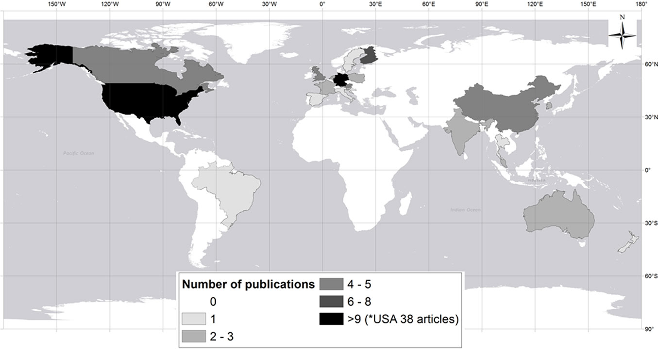
The analyzed studies were carried out in 25 countries on all continents, except Africa and Antarctica. Most papers were performed in the United States (38 papers), followed by Germany (9 papers), Finland (8 papers), and the United Kingdom (5 papers - Fig. 1). This distribution reflects the general number of studies performed on urban forestry worldwide. As reported by Bentsen et al. ([9]), in the principal journal in this subject area, Urban Forestry and Urban Greening, 59% of papers in the years 2000-2008 were performed in North America and Scandinavia.
Fig. 1 - Number of publications per country, retrieved in the Scopus® and ScienceDirect® databases. (*): The number of papers published in Polish magazines was 12.
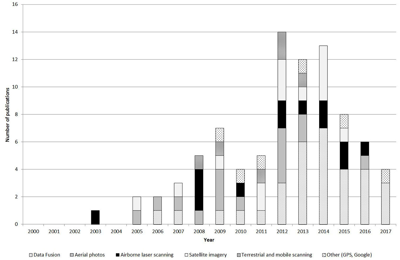
The number of scientific papers whose focus is the determination of greening parameters has trended upward over time. The increase has been shown to be a result of improved access to RS data acquisition technologies; the growth of forestry-focused scientific research, the results of which can be used for analyses of greening in urbanized areas (see Fig. S1 in Supplementary material); and the increased availability of spatial data, resulting from the creation of free-of-charge spatial data repositories ([6], [13], [102], [37]). A diverse range of RS technologies have been developed to determine individual tree parameters and forest stand characteristics (Fig. 2). Since 2010, data from laser scanning has been acquired in multiple studies (ALS and TLS: 19 published studies). Researchers have also often performed analyses from the acquisition and combination of several sets of spatial data (data fusion, DF: 32 published studies).
Fig. 2 - Number of publications retrieved from Scopus® and ScienceDirect® databases per year and the remote sensing technology used.
Accuracy of tree attributes determined using remote sensing
Position
The identification of individual tree positions by means of RS requires two parameters to be defined precisely, i.e., individual tree detection and trunk location (X, Y - Tab. 1). ALS data have predominantly been used for the detection of individual trees, and have been processed using the following algorithms: the tree climbing algorithm ([107]), individual tree detection (ITD - [27]), and watershed segmentation (crown-level fusion of hyperspectral imagery and ALS data - [2]). Individual tree crowns have been delineated using canopy height models ([89]), image segmentation ([68]), local maxima algorithms (LMA), and the Koukoulas and Blackburn algorithm (KBA - [77]), as well as a variable window filter ([69]). The accuracy of detection ranged from 69% (KBA method) to 99% (variable window filter method).
Tab. 1 - Selected scientific publications reporting individual tree detection, tree height, DBH, and crown parameters. The research area, data set, method and accuracy are reported. (-): this variable was not specified; (n/d): this variable was specified but no error was given.
| Publication | Study Area | Data Set | Method | Single tree detection rate | X,Y Coordinates accurancy and precision | Tree height prediction results | Tree crown parameters prediction results | DBH prediction results |
|---|---|---|---|---|---|---|---|---|
| Shrestha & Wynne ([81]) | US | DF (ALS, satellite imagery) | Manual (acquiring information from a raster) | - | - | 1.34 m (RMSE); 0.89 (R2) |
0.75 (RMSE) 0.9 (R2) | 0.11 (RMSE) 0.82* (R2) |
| Lee et al. ([43]) | US | DF (ALS, satellite imagery) | Regional maxima,manual | - | - | 1.64 m (RMSE); | 1.07 m (RMSE) | 0.10 m (RMSE); 0.88 (R2) |
| Zhang & Qiu ([107]), [109]) | US | DF (ALS, hyperspectral imagery) | Tree climbing algorithm | 93.5% | - | 0.57-1.11 m (RMSE); 0.93-0.98 (R2) | 0.63-0.84 (R2) |
- |
| Phu La et al. ([68]) | US | DF (ALS, hyperspectral imagery) | Image segmentation | 62.0-70.0% | - | 0.45-0.97 (R2) | 0.26-0.96 (R2) |
- |
| Alonzo et al. ([2]) | US | DF (ALS, hyperspectral imagery) | Watershed segmentation | 83% | - | - | - | - |
| Banzhaf & Kollai ([7]) | Germany | DF (Orthophotos, ALS) | Geographic Object Based Image Analysis (OBIA) | n/d | - | - | - | - |
| Iovan et al. ([31]) | France | DF (Orthophotos, ALS) | SVM / obust region growing algorithm based on tree-shape criteria | 78% | - | - | - | - |
| Saarinen et al. ([80]) | Finland | DF (ALS, TLS) | Watershed segmentation/Visual interpretation | - | 0.1 m (bias) |
-1.0-1.0 m (difference) | - | 0.39-0.76 m (RMSE) |
| Tompalski ([94]) | Poland | DF (TLS, ALS, satellite imagery) | Voxel-Based Method /Convex hall/LasBoundary algorithm | - | - | 1.77 m (RMSE); 0.94 (R2) |
0.46-0.56 (R2) |
0.03 m (σ) |
| Holopainen et al. ([27]) | Finland | DF (ALS, TLS, MLS) | Individual Tree Detection/ cylinder fitting | 73.29- 79.22% | 0.44-1.57 m (RMSE) | - | - | - |
| Plowright et al. ([69]) | Canada | ALS | Variable window filter | 99.0% | - | 1.09 m; 0.93 (R2) |
- | - |
| Rahman & Rashed ([77]) | US | ALS | KBA/LMA | 69.0-73.0% | - | 0.81 - 0.87 (R2) | - | - |
| Tanhuanpää et al. ([89]) | Finland | ALS | Watershed segmentation | 88.8% | 0.25 m (bias) |
1.27 m (RMSE) | - | 0.07 m (RMSE) |
| Wu et al. ([101]) | China | TLS/MLS | Voxel-Based Method | 98.5 - 100% | - | - | 0.92-0.93 (R2) |
0.03 m (RMSE); 0.87 (R2) |
| Vonderach et al. ([99]) | Germany | TLS/MLS | Voxel-Based Method | - | - | 0.5-1.6 m (difference) | - | -0.01-0.08 m |
| Moskal & Zheng ([55]) | US | TLS/MLS | Point Cloud Slicing (PCS) | - | - | 0.75 m (RMSE); 0.57 (R2) |
- | 91.0%; 0.09 m (RMSE) |
| Rutzinger et al. ([79]) | Holland | TLS/MLS | 3D Modelling | 86.0% | - | n/d | - | - |
| Tompalski ([93]) | Poland | TLS/MLS | Convex hulls | - | 0.57 m (bias) |
2.27 and 1.58 m (σ) | -0.35 m (bias) |
- |
| Ardila et al. ([5]) | Holland | Satellite imagery | Geographic Object Based Image Analysis (OBIA) | 70-82% | - | - | - | - |
| Morgenroth & Gomez ([53]) | New Zealand | Digital photographs | Photogrammetric stereo-measurements conducted on digital photographs taken on the ground level | - | - | 0.1 m | - | 0.03 m (bias) |
| Patterson et al. ([67]) | US | Digital photographs | Manual measurements in UrbanCrowns software application | - | - | n/d | n/d | n/d |
High spatial resolution satellite imaging is an alternative to laser scanning for tree species group detection. Ardila et al. ([5]) achieved 70% to 92% accuracy in species detection, depending on the study area, with the use of QuickBird satellite imaging. The error of commissioning associated with this technique was equal to 26% (mainly for single trees with a crown area < 15 m2), and the error of omission ranged from 18% to 30%. Apart from the method used, the character of the research area also impacted on the reliability of results, which varied with, among other factors, dominant species type (deciduous/coniferous), tree age, and quality of reference data ([85]). Plowright et al. ([69]), who achieved the most accurate detection results, used the variable window filter algorithm in their research, which, prior to that study, had mainly been applied to forest areas ([71], [85]), where the parameters of the tool were calibrated in accordance with species composition and age/height of the forest. In Plowright et al. ([69]) research, the method was calibrated against a single species, but also indicated that it is possible to develop equations for other tree species and apply them in parallel. Rahman & Rashed ([77]) showed that combining the LMA and KBA methods generates more reliable results than using these methods separately. The improvement in results is due to the limitation of the KBA algorithm in identifying and measuring the height of individual trees and groups of trees, being overcome by the LBA algorithm which has the ability to identify individual trees with overlapping canopies. Tanhuanpää et al. ([89]) pointed out that the time of data acquisition has an impact on the obtained results, in that if the reference data (field data) and RS data were obtained on different dates, some trees may have been removed, planted or replanted. In this case, attention should be paid to data cohesion. The main reasons for that are a wide range of species (many non-native species), and spatial/structural variability (e.g., single tree growth, varying light conditions, and tree shape modification by human activities). A large variation in the size and shape of tree crowns forces the user to choose between the algorithms generating too many or too few trees during segmentation.
The problem of reference data quality from GIS urban databases was emphasized by Plowright et al. ([69]), who showed the importance of improving coordinate accuracy derived from RS databases, by correcting positional errors, and removing trees that may have been incorrectly recorded. Moreover, Tanhuanpää et al. ([89]) pointed out that substantial problems in individual tree detection are caused by the diversity of tall objects in the urban environment, which confuse the algorithms used to detect vertices; for example, lamp posts, power lines, and tall vehicles in the streets. Such issues present different challenges for researchers involved in the detection of trees in urban environments, compared to studies that detect trees in forest areas ([89], [109]). Ardila et al. ([5]) pointed out that aerial images collected during leaf-off conditions are usually subject to geometric distortions that affect the accuracy of tree surface estimation, but are only occasionally used. They also emphasized that the urban environment is more diverse than forest areas; in forests, the picture is less complex and the adoption of specific parameters in Geographic Object-based Image Analysis (GEOBIA) generates results with a similar degree of accuracy in different areas. ITD methods are available and in general give acceptable results for urban greening inventories. ALS data are the most reliable, and multispectral data are adequate for this purpose. Integration of the various RS data, where possible, improves the accuracy of results. Most authors agreed that the urban environment is more complex that the forest environment, which causes many additional problems in the detection of individual trees.
Tompalski ([93]) processed TLS data using the method of convex hulls generated at certain heights over the ground surface, and found the position of trees was set with an average error of 0.57 m. More accurate results, with an average error of 0.10 m, were obtained by Saarinen et al. ([80]), who applied a visual interpretation method. Holopainen et al. ([27]) compared the accuracy of determining tree trunk positional coordinates by TLS, MLS, and ALS. The results of the study showed that TLS data reproduced tree position with the best accuracy, where root mean square error (RMSE) was equal to 0.12 m; whereas MLS data had a RMSE = 0.36 m, and ALS data a RMSE = 1.27 m. In the opinion of Holopainen et al. ([27]), the error in tree position estimates based purely on ALS data is caused by the variation in crown shapes as well as the age of trees, which influences the size of the crown. The accuracy of tree positions determined from ALS data in urban environments is similar to the results obtained in forest areas by Kaartinen et al. ([34]). The results of these studies show that one advantage of TLS and MLS data is the high accuracy with which tree position can be determined, even for those growing under dominant trees. ALS data is associated with larger errors, but the cost of data acquisition is much smaller than for MLS and TLS. ALS data are abundant and easy to access. MLS and ALS have high operationality. The TLS technique is more suited to small area inventories that require very high precision.
Tree height
There are three methods that can be used to extract information on tree height from RS data: (i) point cloud processing of data collected using active LiDAR technology (ALS, MLS and TLS); (ii) stereophotogrammetric measurements extracted from digital photographs taken at ground level; and (iii) 3D point cloud processing using airborne digital image matching. A precise digital terrain model, which can be created from ALS data, is a requirement of the latter method. So far, studies using 3D point cloud processing are rare.
The accuracy of tree height measurements retrieved from ALS depends on factors such as flight and data acquisition parameters, tree species being measured, data processing technology, and the method used for individual tree identification ([84]). Tanhuanpää et al. ([89]) applied an ALS point cloud with a density greater than 20 pts m-2. The accuracy achieved with the watershed segmentation method (RMSE = 1.08 m) was comparable to the accuracy achieved by Rahman & Rashed ([77]) using the KBA method (RMSE = 1.08 m), and the LMA method (RMSE = 1.3 m). The LMA method was also used by Plowright et al. ([69]), who achieved a mean error in height measurements equal to 1.09 m, using a point cloud density equal to 25 pts m-2. Zhang et al. ([109]) performed treetop detection using a constrained tree climbing algorithm, and achieved accuracies ranging from 0.47 to 1.11 m (RMSE). The relatively low error achieved in Zhang et al. ([109]) may result from the fact that most trees in the study area were broadleaved with a wider top than conifers, which increased the probability that laser pulses hit the treetops. Shrestha & Wynne ([81]) presented height measurements for 9 tree species with an average RMSE value of 1.34 m.
Vonderach et al. ([99]) showed that height determined from TLS data is regularly underestimated. The differences in TLS measurements and terrestrial measurements fall within a range of 0.50 to 1.50 m. Similar results, with an RMSE equal to 1.77 m, were achieved by Tompalski ([94]). With MLS, Wu et al. ([101]) determined tree heights with an R2 coefficient of 0.9, and an RMSE equal to 0.18 m. Morgenroth & Gomez ([53]) used a point cloud generated from ground level digital photographs taken from multiple positions. In their studies, tree height estimates contained an error of 0.10 m (2.59%).
The accuracy of tree height measurements using ALS data depends not only on data processing methods but also on the tree species, and is also dependent on the quality of field-based measurements ([50]). Their results show that when relatively high point density ALS data are used, the error in height estimation is greater for some deciduous species (e.g., oaks) than for conifers and alder. This is not related to the reliability of ALS measurements, but rather to the difficulty associated with precisely measuring the height of old trees, such as oaks. Oak crowns are usually irregular and complex; therefore, it is difficult to clearly determine the top of the tree from the ground. Measuring the height of conifers is easier and more precise due to their compact and cone-shaped crowns. Mielcarek et al. ([50]) also noted that errors for deciduous trees increased slightly with increasing tree height. Such a tendency was not found in coniferous and alder trees. Further, ALS data itself can influence height measurements. Morsdorf et al. ([54]) proved that the underestimation of tree heights by ALS increased by approximately 0.3 m with an increase from 500 to 900 m flying altitude. Yu et al. ([105]) showed that tree height could be measured more accurately with a large footprint, because the laser pulse has a higher probability of hitting the top of the trees. Tanhuanpää et al. ([89]) and Orka & Bollandsås ([63]) determined that ALS should be collected during the leaf-on season, because the data generates less noise and lower errors than leaf-off data, which can be explained by the denser canopy under leaf-on conditions. Tompalski ([94]) showed that there was no relation between the height of a tree measured using TLS and the distance of a tree from the scanner, or the height of a tree and other features, such as the type and number of points. Contrasting results were achieved in a forest area by Olofsson et al. ([62]), who proved that the error in tree height measurements depends on distance to the scanner. According to Tompalski ([94]), scanning in unfavorable terrain with a high density of trees does not prevent the acquisition of exact tree height values. Tompalski ([94]) also indicates that scanning should be performed during the leaf-off period, and the number and distribution of scanning positions should be properly arranged.
Diameter at breast height
Previous studies have reported three different approaches for the determination of the diameter at breast height (DBH). The first involves the use of descriptive variables from ALS data, the second uses TLS and MLS data and the third is based on a cloud of points that are generated from photographic images. Shrestha & Wynne ([81]) determined DBH with an indirect method using two types of ALS variable. DBH determined from tree crown size resulted in R2 coefficients of 0.82 for all trees, 0.84 for deciduous species, and 0.74 for coniferous trees. Assessing DBH based on average height resulted in inferior R2 coefficients, i.e., 0.72 for all trees, 0.76 for deciduous species, and 0.54 for coniferous species. By constructing convex hulls from TLS data, Tompalski ([93]) achieved DBH estimates with an RMSE of 0.013 m and a standard deviation of 0.03 m. Using a point cloud slicing (PCS) method based on voxel data structure and circle fitting, Wu et al. ([101]), Moskal & Zheng ([55]), and Vonderach et al. ([99]), achieved accuracies in DBH estimations of 0.03 m (RMSE), 0.09 m (RMSE), and -0.01 - 0.08 m (bias), respectively. Results achieved by Vonderach et al. ([99]) are similar to Tompalski ([94]). With a point cloud constructed from a series of digital photographs, Morgenroth & Gomez ([53]) calculated a DBH for an individual tree with an error of 0.03 m. As Wu et al. ([101]) emphasized, despite the high quality of results, TLS data have limited application in urban areas, due to the limited coverage that can be achieved from TLS devices. This strongly contrasts with ALS data collection methods. According to Tompalski ([94]), the circle fitting method is the most reliable, because it works better when trunk cross-sections are only partially covered by points. However, a large number of alternative solutions exist in the literature that have not yet been tested in an urban environment ([74]). Results can also be improved by performing single or multistation scans, which construct more accurate reproductions of breast height ([94]).
Tree crown
The subject of determining the parameters of the crown is often not addressed in scientific publications. In studies where this issue is considered, parameters were estimated directly or indirectly from ALS, MLS, or TLS data, or from field-based photos. Using ALS data, Shrestha & Wynne ([81]) determined crown spans with an R2 coefficient of 0.90. Crown diameters were calculated in that study from ALS data using the formula: 2 · radius = √crown area /π, with a RMSE of 0.75 m. In the same study, a lower correlation (R2 = 0.75) was achieved by calculating maximum heights and crown span values from field measurements. Zhang et al. ([109]) using ALS data identified the height of tree crown bases with a correlation (r) value of 0.63-0.84, and a crown span with R2 values ranging from 0.7 to 0.84. With ground level laser scanning, Tompalski ([94]) calculated crown projection surfaces with an R2 coefficient of 0.81. Tompalski ([93]) determined crown base height with a mean error of -0.35 m. MLS data was used by Wu et al. ([101]) to determine crown spans with R2 values ranging from 0.92 to 0.93. Abd-Elrahman et al. ([1]) explored the effectiveness of using different digital camera models to assess crown span and crown base height. Based on photographs, the errors in crown span and crown base height values were determined to be 0.4 m and 0.05 m, respectively. Accurate calculation of the crown size parameter is vital for determining crown coverage, which is one of the parameters that characterize the urban ecosystem. According to previous studies, crown size estimated from ALS data is usually less accurate than tree height ([23], [71]). Low accuracy can result from crown shape, low scanning density and the overlap of the crowns of adjacent trees ([109]). The results obtained by Zhang et al. ([109]) were promising, and show that the accuracy of key parameter estimates, such as base height and depth of the crown, may be related to the accuracy of tree height estimates. This is important because, even during field measurements, it is difficult to measure such parameters, especially in densely forested areas. Zhang et al. ([109]) suggested that a higher scanning density may lead to higher accuracy, as the probability of hitting lower branches will increase.
Health condition
The majority of studies concerning vegetation health condition were performed using aerial (including hyperspectral) and satellite imagery. A number of authors ([26], [25], [29], [108], [70]) compared the health condition of healthy, diseased and dead trees with vegetation indices, or determined relationships between the variables obtained from RS data and biophysical variables (e.g., defoliation and discoloration). Malthus & Younger ([45]) determined the correlations between an overall tree condition index (OTC), defoliation, and selected vegetation indices, such as the Normalized Difference Vegetation Index (NDVI), the Green Normalized Difference Vegetation Index (gNDVI), and the red edge position (REP). A significant correlation was only observed between the OTC and the gNDVI, and the OTC and the REP. The authors did not find any relation between the defoliation and vegetation indices. Xiao & McPherson ([103]) carried out an analysis of tree health at the two scales of individual tree and individual pixels. The authors classified trees as healthy if the ratio of healthy pixels determined by NDVI and the total number of pixels was higher than 70%; otherwise, trees were classified as unhealthy or dead. The total accuracy of classification on the level of individual trees was 88.9%, i.e., 86% for deciduous trees and 91.0% for coniferous trees. Holopainen et al. ([26]) used aerial color infrared imagery to assess the volume of trees damaged as a result of drought. They achieved their results by visual interpretation of the images. Jarocinska et al. ([32]) applied the Photochemical Reflectance Index (PRI) and the Normalized Difference Vegetation Index (NDVI705) to determine discoloration and defoliation, respectively. Their results showed R2 coefficient values of 0.43 and 0.44, with RMSE ranging from 11% to 23%. The analysis was performed using satellite imagery from the beginning of July until the end of August. Jarocinska et al. ([32]) showed that it was feasible to estimate the health condition of urban forests by analyzing the values of vegetation indices, defoliation and discoloration. Hanou ([25]), Zhang et al. ([108]), Hu et al. ([29]), and Pontius et al. ([70]) described the use of various datasets and methods to identify ash trees and determine their health status. The need for this kind of analysis emerged from the large scale damage caused by the activity of the emerald ash borer (EAB - Agrilus planipennis Fairmare). Hanou ([25]) proved that there is a correlation between hyperspectral signatures and the level of infestation measured by the gallery counts per square meter of measured material or trunk. Zhang et al. ([108]) estimated the EAB infestation stages of a single ash tree by using various types of spatial data (hyperspectral and satellite imagery). To achieve this, they used three input variables: the leaf chlorophyll content, tree crown spatial pattern, and prior knowledge. The overall accuracy (OA) was 62.5%, with an omission error of 22.5%, and a commission error of 18.5%. Based on vegetation indices sensitive to leaf chlorophyll content, Hu et al. ([29]) confirmed that the amount of chlorophyll measured by vegetation indices is capable of predicting the presence or absence of the EAB in ash trees. The OA of the binary classification used in that study (healthy/infected) was 70%. It should be mentioned that the authors used a limited number of 33 ash trees for the training and test samples. The health condition of ash trees was estimated by Pontius et al. ([70]), in which identification accuracy ranged from 62% (for the healthiest trees) to 22% (the second healthiest out of five classes). To reduce classification error, they developed multiple endmembers and a spectral unmixing technique to overcome the challenges posed by classification of spectrally complicated study objects situated in an urban environment. An attempt to estimate the health condition of trees from ALS was also performed by Plowright et al. ([69]). Their estimates of crown density had an R2 coefficient of 0.62 for trees over 8 meters high, 0.28 for trees between 5 and 8 m, and 0.001 for smaller trees. The authors applied a coefficient of height variation (CV) as a predictor of crown density (Tab. 2).
Tab. 2 - Selected scientific publications reporting tree health condition using remote sensing data. (UA): user accuracy; (OA): overall accuracy; (*): Determination of health condition through variables.
| Publication | Study Area | Data Set | Sensor | Method | Date of RS data acquisition | Health Condition* | Accuracy |
|---|---|---|---|---|---|---|---|
| Zhang et al. ([108]) | Canada | DF (hyperspectral imagery, aerial imagery) | ProSpectTIR-VS2/Google Earth imagery | Vegetation indices, leaf chlorophyll content, longitudinal profiles, | July 2010 | Healthy/ High/medium/ low condition | 62.5% (OA) |
| Hu et al. ([29]) | Canada | DF (ALS, hyperspectral imagery) | 9 and 4 bands/ ALS (1 pts./m2) | Individual tree crown | 2009, ALS- summer 2007 | Healthy/unhealthy (1 species - Ash) | 70% |
| Pontius et al. ([70]) | US | DF (ALS, hyperspectral imagery, thermal imagery) | GLiHT | Segmentation | June 2006 | 4 vigor classes | 0-62% |
| Plowright et al. ([69]) | Canada | ALS | Leica ALS70-HP (25 pts./m2) | Crown density as the response variable and the percentage of non-ground LiDAR returns and the coefficient of variation of return heights as separate predictor variables | April 2013 | Crown density | 0.62 (R2) for trees in 8 m to 14 m height class |
| Hanou ([25]) | Canada | Hyperspectral imagery | ProSpectTIR-VS2 | Gallery Count / Area (DBH) | July/August 2010 | Low/medium/high Emerald Ash Borer | 0.8 (R2) |
| Malthus & Younger ([45]) | UK | Aerial imagery | CASI | Correlation between: Visual Stress Index (leaf colour × crown density); General Crown Condition Index (crown die-back × crown density × Leaf size × number of small dead limbs); Foliage Index (foliage colour × degree of leaf chlorosis × degree of leaf necrosis); Overall Tree Condition Index (a combination of the first threeindices prior to equilibration, summed and then normalised) and vegetation indices | September 1996 | Defoliation and OTC index for 4 species | -0.14 - -0.83 (correlation) |
| Xiao & McPherson ([103]) | US | Aerial imagery | Wild RC10 | Vegetation indices (NDVI) | Summer 2003 and 2004 | Classification (healthy/ unhealthy) |
88.9 % |
| Holopainen et al. ([26]) | Finland | Aerial imagery | - | Photointerpretation | July 2003 | Assessing the volume of trees damaged as a result of drought | - |
| Jarocinska et al. ([32]) | Poland | Hyperspectral imagery | HySpex | Correlation with vegetation indices | July and August 2015 | Discoloration | 0.43 (R2) |
| Defoliation | 0.44 (R2) |
Tree species
The identification of tree species by RS is a complex issue due to the large diversity of species in urban areas. Trees are classified either on the single tree (object) or the pixel scale. When single tree classification is carried out, ALS- (image-)based single tree detection is usually performed first, and then segments are classified based either on spectral (image) or structural (point cloud) data, or both variables. Typically, RS data fusion is utilized for species classification. The first studies incorporating Google™ Street View® (GSV) images have begun to appear in the literature. The global scale of the Google™ image database is expected to revolutionize the study of urban greening (Tab. S2 in Supplementary material).
In the most complex urban ecosystems, Alonzo et al. ([2]) performed classification analyses of 29 dominant tree species. The study used hyperspectral imagery with ground resolution 3.4 and 3.7 m and ALS data with resolutions of 22 pts m-2. The OA of classification for the 29 dominant tree species was 83.40% (κ= 0.82). The application of ALS-based variables to the classification model improved the OA by approximately 4.20%. Zhang & Qiu ([107]) classified 40 species and achieved an OA of 68.80%. The difference in OA values between the studies was caused in part by the different number of tree species classified, and more importantly the fact that the point clouds generated from ALS data had very different densities (22.0 vs. 3.50 pts m-2). Since ALS-based variables are fundamental to tree classification methods ([35]), denser point clouds provide better descriptions of tree structure and significantly improve classification results.
Voss & Sugumaran ([100]) performed classification of seven tree species using two sets of hyperspectral data from the summer and fall season, combined with ALS data. The determination of tree species was carried out using an object-oriented classification with two variants. The first variant used information from hyperspectral imagery (after minimum noise fraction, MNF, transformation), and the second used additional information from ALS (intensity and height). The OA of classification in the first variant was 48% for summer data, and 45% for fall data. In the second variant with additional ALS data, the general accuracy increased to 57% and 56%, respectively. A 19 percentage point increase in OA values was achieved by the incorporation of ALS data in Liu et al. ([44]). However, Ghosh et al. ([21]) reported no improvement in results, although they used tree heights calculated exclusively from ALS data.
Dian et al. ([17]) combined hyperspectral data (10 most informative channels after MNF transformation), the Enhanced Vegetation Index (EVI), and ALS data (the normalized Digital Surface Model and segments of individual tree crowns), achieving a general classification accuracy of 79.20% (κ = 0.68). Jarocinska et al. ([32]) attempted to identify 12 tree species in the area of Bialystok (Poland). The classification was carried out on the 40 most informative channels of hyperspectral imagery (MNF transformation), using the spectral angle mapper (SAM) method. Total classification accuracy was 78.80% (κ = 0.69). Pu & Landry ([73]) classified 7 tree and tree group species using IKONOS and WorldView-2 satellite imaging. The general classification accuracy for the method was 56.98% (κ = 0.48) based on IKONOS data, and 62.93% (κ = 0.42) for WorldView-2 data. The authors developed a stepwise masking protocol to distinguish between sunlit and shaded tree canopies, and they compared the accuracy of tree species mapping between four-band IKONOS imagery and three different band combinations of WorldView-2 imagery (four “traditional” bands, four additional bands, and all eight bands). Latif et al. ([42]) used World-View 2 data to perform a classification of 8 species using the minimum distance algorithm. They achieved a user’s accuracy (UA) of 0-87.2% for the individual species. Tooke et al. ([95]) used QuickBird imagery and information about shaded areas obtained from ALS data. They used the decision tree classification algorithm and linear spectral mixture analysis (SMA) to distinguish between low and high vegetation, and then between coniferous and deciduous trees with different health conditions (manicured and mixed). Verlič et al. ([98]) combined ALS data and satellite imagery (WorldView-2), to determine five different species using example-based feature extraction (ENVI 5 software), by applying the support vector machine (SVM) model, and achieved a UA from 12% (sweet chestnut) to 69% (Norway spruce). Tigges et al. ([92]) performed the classification of the eight species that are considered to be dominant in Central Europe, by testing different spectral and temporal band combinations of five RapidEye images that were collected during the vegetation season. To improve the results, they used ancillary surface and terrain models. The UA of each classification depended on the tree species and varied from 66% to 99%. Berland & Lange ([10]) used GSV materials to identify tree species. In their study, a botanic specialist identified tree species based on GSV pictures, and if the identification of tree species was not possible, the type of tree was identified. Furthermore, results were compared with data from field measurements. The classification accuracy was 66% on the level of species and was 90% on the level of genus.
It is almost impossible to compare results that were obtained in different studies because there are too many differences between the study sites, the total number of species and the time when data was collected. In Xiao et al. ([104]) work, a method called the Number of Categories Adjusted Index (NOCAI) was used to compare different papers. The NOCAI is calculated by dividing the accuracy that was achieved by a specific algorithm to give an expected accuracy that would be obtained if trees were randomly assigned to a species. The expected accuracy is simply 1/k·100%, where k is the number of species. The NOCAI was applied to works using ALS and hyperspectral data, with the highest NOCAI value (27.52) being achieved by the algorithm developed by Zhang & Qiu ([107]). Tigges et al. ([92]) reported that NOCAI values of 6.84 for studies that only used ALS and satellite data for classification. The most accurate results regarding tree species was obtained by combining hyperspectral imagery and ALS data during analysis ([107], [100]). As shown by previous studies, the combination of these datasets can be used to perform both pixel- and object-based classifications. A pixel-based approach enables classification results with errors from 5.10% to 18.80% (OA) to be achieved, which is better than results obtained by analyzing single format data ([44]). It should be noted that in a single tree crown, the leaf-level spectral reflectance may vary with leaf biochemistry and water content. Dian et al. ([17]) noted that the variability in a class may be greater than between classes. For hyperspectral data this is not the case, since lower GSD data area used because of the high cost of acquisition. To obtain the best results two strategies should be implemented: either hyperspectral data (which enlarges spectral information), or multispectral data with ALS data (to compensate for the lack of spectral information), should be combined with structural information from ALS data. Hyperspectral and ALS data are currently the best possible combination of RS data for species classification.
The season in which data were obtained had an impact on the accuracy of the species classification. Voss & Sugumaran ([100]) achieved better classification results using data collected in summer (OA = 48% without ALS; OA = 57% with ALS) rather than in autumn (OA = 45% without ALS; OA = 56% with ALS), although the difference was small (3% without ALS, 1% with ALS data), and had no practical meaning. According to Liu et al. ([44]), the most important parameters for detecting tree species during the spring budburst stage were the Anthocyanin Content Index and the Photochemical Reflectance Index. The most widely used classification algorithms include the SVM, the SAM, the random forest (RF), and the maximum likelihood (ML). Accurate results were generated by all algorithms, but due to the diversity of study sites, number of classified species, number of reference data used, and the fusion of various types of RS data acquired at different times of the year, it is impossible to identify which algorithm is most advantageous ([19]).
Opportunities and limitations of individual remote sensing technologies
From the point of view of public administration, the information regarding individual tree position is one of the most important attributes acquired during inventories. Detailed location information constitutes the basis for the efficient planning of greening resources (cutting/planting), and the construction of ground and terrestrial infrastructure ([65]). The content of inventory maps produced from these data is often essential to making administrative decisions. According to the technical standards set by the Ministry of Internal Affairs and Administration in Poland regarding the execution of detailed surveys, single trees, as well as parks, squares, and lawns, are classified as Group II situational points. This classification requires that their location on maps should be specified within 0.30 m accuracy, in relation to geodetic control network points, before results can be added to the National Geodetic and Cartographic Database ([48]). According to published studies, it is possible to identify tree locations to this level of accuracy with TLS, but MLS and ALS data do not currently meet this requirement. Many of the tenders offered by local authorities include unspecified entries, e.g., the “identification of trees and bushes in the area of […] in order to include their specific position in an inventory map” ([28]). In the authors’ opinion, such an entry allows the application of TLS or ALS techniques to acquire information on tree locations with an error defined in the subject literature. Tender documents (for example, in Poland) related to urban forest inventories indicate that height and crown diameters should be measured to an accuracy up to 0.50 m and 1.00 m, respectively, and a breast height diameter with an accuracy of 0.01 m. The results of the literature reviewed here show that TLS data can be used to determine all parameters with the required accuracy ([99]). MLS technology can be used to accurately measure crown span and height, but the accuracy required for DBH of up to a few centimeters may not be sufficient for end users ([101]). Zhang et al. ([109]) showed that it is possible to measure tree height with an RMSE value of 1.11 m with ALS (calculated against field based measurements). If one takes into account the error of 0.45 m associated with manual field measurements, the resulting error in height measurements derived using the ALS method will be approx. 0.7 m. In reality, this value can be lower, since high density ALS data (which is often acquired over cities) usually records heights that are very close to the real height of trees. The error will be within the range of practitioners’ requirements. ALS data may also be used as an alternative source of data for crown span measurements. It is not possible to measure DBH directly using ALS methods, and assessment of DBH via indirect methods is too imprecise to constitute a substitute source of reliable data ([81]). The optimal dataset therefore comprises individual tree positions and geometrical attributes obtained from terrestrial and aerial laser scanning data, tree heights obtained from ALS data, and detailed information about stem quality and precise tree location from TLS data ([89]). It should be noted that no studies were found that discuss the integration of information collected by terrestrial laser scanning and airborne laser scanning. Such studies have been carried out in forest areas ([8]), and it is likely that they could be applied successfully to urban areas.
Tree species is the most important attribute acquired during an inventory ([65]). Urban areas contain a great variety of species; typically, native tree species dominate the urban landscape, accompanied by a mixture of minor non-native species. Alonzo et al. ([2]) indicated that it is possible to classify up to approximately 30 of the most numerous tree species in a given area. From a practical point of view, less numerous species should be classified into an aggregate group, i.e., deciduous/coniferous species. Therefore, substantial limitations remain in regard to the possibility of replacing the field measurement of tree species with information obtained by RS.
RS data enables tree health to be recognized with high accuracy ([103]). A lower accuracy is provided by methods that specify correlations between vegetation indices or variables that are calculated from a point cloud, and parameters such as defoliation or discoloration. As shown by Xiao & McPherson ([103]), RS enables fast acquisition of information regarding the health condition of individual trees within the whole urban area. Information regarding individual trees may be used to plan cutting or replacement planting. Furthermore, the information from individual pixels within crowns may determine the need for tree pruning, watering or carrying out a site survey to determine the cause of damage. Jarocinska et al. ([32]) showed that the use of continuous data, such as RS data, enables greening condition to be differentiated depending on location (e.g., trees along roads are characterized by worse health condition than ones that are at a greater distance). From a practical point of view, it is more important to develop a model that could help detect the occurrence of pathogens at an early stage, so as to minimize negative effects, than to define the pre-existing effects of various factors that have caused deterioration in tree health. Comprehensive data (e.g., age and species) are needed to accurately assess the health condition of trees, and parametrize models effectively. The unavailability of such data may decrease the effectiveness of ALS data in determining tree health conditions, since for example height information from ALS can be used as a proxy for tree age. It is not possible to identify damage factors (e.g., fungal pathogens) from RS data, but it is possible to determine the general condition of trees (e.g., good, average, poor), which may constitute the basis for further field investigations. The accuracy of assessing selected tree attributes from different data sets is presented in Tab. 3. The authors evaluated the results in the literature according to the following guidelines: Grade 0: no data; Grade 1: R2 ≤ 0.5 or accuracy ≤ 50%; Grade 2: 0.5 < R2 ≤ 0.7 or 50% < accuracy ≤ 70%; Grade 3: 0.7 < R2 ≤ 0.9 or 70% < accuracy ≤ 85%; Grade 4: R2 > 0.9 or accuracy > 85%. The compatibility of information from different data sets constitutes the other factor to be considered when selecting RS data for inventories.
Tab. 3 - Accuracy evaluation of specific tree parameters (Grade 0: no data; Grade 1: R2 ≤ 0.5 or accuracy ≤ 50%; Grade 2: 0.5 < R2 ≤ 0.7 or 50% < accuracy ≤ 70%; Grade 3: 0.7 < R2 =< 0.9 or 070% < accuracy ≤ 85%; Grade 4: R2 > 0.9 or accuracy > 85%). The listed number of publications is reported in brackets. Last column shows the number of parameters (attributes) which could be measured using the corresponding method.
| Data/Method | Location | Tree height | DBH | Crown span | Height of tree crown basis | Crown projection surface | Species | Health condition | Total Attributes |
|---|---|---|---|---|---|---|---|---|---|
| Aerial imagery | - | - | - | - | - | - | 4 (4) | 1-3 (5) | 2/8 |
| ALS | 4 (3) | 4 (3) | - | - | 3 (1) | - | 0 (1) | 2 (1) | 5/8 |
| DF (ALS, TLS/MLS) | 3 (1) | 4 (1) | - | - | - | 0 (1) | - | - | 3/8 |
| DF (ALS, Hyperspectral imagery) | 4 (3) | 4 (2) | - | 4 (2) | 4 (1) | - | 1-4 (10) | 2-3 (3) | 6/8 |
| DF (ALS, Satellite imagery) | 3/4 (1) | 3/4 (2) | 3 (2) | 4 (2) | - | - | 1-4 (2) | - | 5/8 |
| DF (TLS, ALS, Satellite imagery) | - | 4 (1) | - | - | 2 (1) | 3 (1) | - | - | 3/8 |
| Other (GSV) | - | - | - | - | - | - | 2 (1) | - | 2/8 |
| Digital photographs | 4 (1) | 4 (1) | 4 (2) | 4 (1) | 4 (1) | - | - | - | 5/8 |
| TLS/MLS | 4 (3) | 4 (4) | 4 (3) | 4 (1) | 4(1) | - | - | - | 5/7 |
| Satellite imagery | 3 (1) | - | - | - | - | - | 2 (2) | - | 2/7 |
In studies that applied data fusion, the authors, depending on the purpose of their studies, did not always have to assess all of the attributes that are listed in Tab. 3. Therefore, based on the results of this literature review and the compatibilities of individual data items, it can be concluded that complete information regarding the eight listed attributes may be obtained using terrestrial or airborne laser scanning and airborne photography (hyperspectral). Data selection should also depend on field based data and available financial resources. Holopainen et al. ([27]) suggested that TLS measurements, due to their cost and labor consumption, should be performed only in environmentally significant areas, where a more accurate assessment of tree parameters other than location is required. The application of MLS is reasonable for trees that are growing in the vicinity of roads or in parks. Airborne data should be collected to compile inventories over the area of a district or a city.
Remote sensing data collection methods have their limits. Above all, the data are relatively expensive and require sophisticated methods of processing by specialists. Public administration in city level currently lacks the specialists and software which allow large datasets to be processed automatically. Many of the publications in this review use sophisticated, bespoke processing techniques which are not available as user-friendly software. This is a major constraint on the application of more sophisticated processing and implementation of such technologies to facilitate the determination of more detailed characteristics of single trees. The need for specialist processing results in not only the costs of acquisition, but also data processing costs, being higher, as well as study lengths being longer. The most expensive data are those which enable the highest measurement precision; that is, TLS and MLS. Airborne or satellite data acquisition techniques make it possible to analyze large areas, but the precision of such research is lower ([27]).
The ideal remote sensing technique for data acquisition is dependent on the scale of the analysis. In the case of urban vegetation, the optimal scale of analysis is a single tree, however, many works are performed throughout cities to determine vegetation cover ([24], [52], [96]). Taking into the account the shape and size of tree crowns in urban environments, it is difficult to constrain an optimal ground sample distance for a defined area. In the aforementioned literature, the data densities range from several to several dozens of points per square meter, and spectral data resolution from several dozens of centimeters to dozens of meters. Myint et al. ([57]) suggested that pixel size used to classify objects should be at least half the size of the object, as too many small pixels for a single large object causes large spectral change, making it more difficult to classify the object.
Atmospheric conditions can pose a problem to remote sensing techniques. Remote sensing data acquisition, in order to be useful, must be carried out in optimal light conditions, ideally without wind and with no cloud cover ([33]). In many countries (e.g., Poland) such days, when data acquisition is possible, are limited (30-40% of the year). Cloud cover can make it impossible to acquire data for several weeks. This can have significant negative impacts, considering that in order to acquire accurate classification results, most images need to be acquired in the vegetation period, which only lasts a few months a year.
The remote sensing data market does not appear ready to carry out surveys for a large number of towns, especially if multi-temporal analyses are being considered. Data is acquired at much greater effort in multi-temporal analyses, and much bigger datasets are acquired from single flights. This prolongs the time required for data processing, and thus the research output. In a country with several dozens of big cities, it is practically impossible to acquire RS data more often than once a year for a single city. The ability to collect such data depends on the remote sensing services market in any particular country, the number and availability of hyperspectral scanners, and many other factors related to the acquisition of remote sensing data.
Conclusions
The use of remote sensing data makes it possible to determine the characteristics of urban vegetation at various levels of detail and at different scales. The accuracy of analyses depend on the type and quality of the RS data used, and the environment in which the analyses were carried out.
Laser scanning is a technology that collects the most versatile RS data on the characteristics of trees. TLS has the highest precision of measurement, while ALS has the largest operating system.
Spectral data, in particular hyperspectral data, allow the classification of up to several dozen species of tree in urban areas. The integration of many datasets, particularly spectral data (aerial images and satellite images) and structural data (LIDAR), facilitates the most complex use of RS data and helps to improve tree species classification estimates.
To estimate the largest possible number of significant parameters from RS data, it is necessary to apply data that have been integrated from multiple sources.
The most important research challenges in urban vegetation monitoring (apart from the development of data processing and data integration methods) are identified as refining species classification methods, tree segmentation methods, and methods of determining specific tree characteristics. There are no studies on these topics that have been performed on large datasets, carried out on a wide geographic scale or on a homogeneous set of remote sensing data.
Despite the fact that this review summarized and attempted to compare the results of the different methods and technologies used in the estimation of tree features and species, it is difficult to state clearly which of them are the most accurate. This is mainly due to the enormous variety of data usage, processing methods, ground data volumes and methods of integrating different types of remote sensing data.
At the moment, no “best practice” methodologies for the use of RS in urban forestry do exist. Such guidelines would address issues such as the selection of RS data for specific purposes, or the technical specifications necessary to achieve particular objectives. In addition, there are no dedicated user-friendly applications designed for the use of civil servants, who do not necessarily have extensive knowledge about remote sensing, but are responsible for acquiring spatial information.
Acknowledgements
This article was written under the project (281502 and 240412) financed by the Polish Ministry of Science and Higher Education.
References
CrossRef | Gscholar
Gscholar
Gscholar
Gscholar
Online | Gscholar
Gscholar
CrossRef | Gscholar
Gscholar
CrossRef | Gscholar
Gscholar
Gscholar
Gscholar
Gscholar
Gscholar
CrossRef | Gscholar
Gscholar
Online | Gscholar
Gscholar
CrossRef | Gscholar
Gscholar
Gscholar
Gscholar
Gscholar
CrossRef | Gscholar
Gscholar
Gscholar
Gscholar
Authors’ Info
Authors’ Affiliation
Krzysztof Sterenczak 0000-0002-9556-0144
Department of Geomatics, Forest Research Institute, Sekocin Stary, Braci Lesnej 3, 05-090 Raszyn (Poland)
Corresponding author
Paper Info
Citation
Ciesielski M, Sterenczak K (2019). Accuracy of determining specific parameters of the urban forest using remote sensing. iForest 12: 498-510. - doi: 10.3832/ifor3024-012
Academic Editor
Raffaele Lafortezza
Paper history
Received: Dec 19, 2018
Accepted: Aug 28, 2019
First online: Dec 02, 2019
Publication Date: Dec 31, 2019
Publication Time: 3.20 months
Copyright Information
© SISEF - The Italian Society of Silviculture and Forest Ecology 2019
Open Access
This article is distributed under the terms of the Creative Commons Attribution-Non Commercial 4.0 International (https://creativecommons.org/licenses/by-nc/4.0/), which permits unrestricted use, distribution, and reproduction in any medium, provided you give appropriate credit to the original author(s) and the source, provide a link to the Creative Commons license, and indicate if changes were made.

Web Metrics
Breakdown by View Type
Article Usage
Total Article Views: 50781
(from publication date up to now)
Breakdown by View Type
HTML Page Views: 39572
Abstract Page Views: 5694
PDF Downloads: 4606
Citation/Reference Downloads: 16
XML Downloads: 893
Web Metrics
Days since publication: 2395
Overall contacts: 50781
Avg. contacts per week: 148.42
Article Citations
Article citations are based on data periodically collected from the Clarivate Web of Science web site
(last update: Mar 2025)
Total number of cites (since 2019): 15
Average cites per year: 2.14
Publication Metrics
by Dimensions ©
Articles citing this article
List of the papers citing this article based on CrossRef Cited-by.
Related Contents
iForest Similar Articles
Review Papers
Remote sensing-supported vegetation parameters for regional climate models: a brief review
vol. 3, pp. 98-101 (online: 15 July 2010)
Review Papers
Remote sensing of selective logging in tropical forests: current state and future directions
vol. 13, pp. 286-300 (online: 10 July 2020)
Research Articles
Three-dimensional forest stand height map production utilizing airborne laser scanning dense point clouds and precise quality evaluation
vol. 10, pp. 491-497 (online: 12 April 2017)
Technical Reports
Detecting tree water deficit by very low altitude remote sensing
vol. 10, pp. 215-219 (online: 11 February 2017)
Research Articles
Integrating area-based and individual tree detection approaches for estimating tree volume in plantation inventory using aerial image and airborne laser scanning data
vol. 10, pp. 296-302 (online: 15 December 2016)
Technical Reports
Remote sensing of american maple in alluvial forests: a case study in an island complex of the Loire valley (France)
vol. 13, pp. 409-416 (online: 16 September 2020)
Research Articles
Spectral reflectance properties of healthy and stressed coniferous trees
vol. 6, pp. 30-36 (online: 14 January 2013)
Research Articles
Mapping the vegetation and spatial dynamics of Sinharaja tropical rain forest incorporating NASA’s GEDI spaceborne LiDAR data and multispectral satellite images
vol. 18, pp. 45-53 (online: 01 April 2025)
Review Papers
Remote sensing support for post fire forest management
vol. 1, pp. 6-12 (online: 28 February 2008)
Technical Advances
Detecting mistletoe infestation on Silver fir using hyperspectral images
vol. 7, pp. 85-91 (online: 18 December 2013)
iForest Database Search
Search By Author
Search By Keyword
Google Scholar Search
Citing Articles
Search By Author
Search By Keywords
PubMed Search
Search By Author
Search By Keyword


