Identification and characterization of gaps and roads in the Amazon rainforest with LiDAR data
iForest - Biogeosciences and Forestry, Volume 17, Issue 4, Pages 229-235 (2024)
doi: https://doi.org/10.3832/ifor4295-017
Published: Aug 03, 2024 - Copyright © 2024 SISEF
Research Articles
Abstract
Gap formations in the forest canopy have natural causes, such as bad weather, and anthropic ones, such as sustainable selective extraction of trees and illegal logging, which can already be detected through orbital remote sensing. However, the Amazon region is under frequent cloud cover, which makes it challenging to detect gaps using passive sensors. This study aimed to identify and delimit gaps in the Amazon forest canopy through airborne LiDAR (Light Detection and Ranging) sensor application while testing six different return densities. LiDAR and forest inventory data were obtained over an Amazon rainforest region, defining the minimum area as a forest canopy gap. The point cloud was processed to obtain six return densities with the generation of their respective CHM (Canopy Height Model), which were applied for segmentation and subsequent identification of gap areas and roads. The minimum gap area found was 34 m2, and the Kruskal Wallis test showed no significant difference among the six densities in gap detection; however, road identification decreased as the return density decreased. We concluded that LiDAR data proved promising as point clouds with low return density can be used without impairing gap identification. However, reducing the return density for road identification is not recommended.
Keywords
Forest Canopy Gaps, Aerial Laser Scanning, Point Density, Remote Sensing
Introduction
Rainforests are subject to natural disturbances of varying intensity, duration, and frequency, making these ecosystems in a continuous and dynamic change ([11]). Forests undergo periodic disturbances (such as fires, strong winds, intense storms, or simply senescence and falls of large trees) that open different-sized gaps in the canopy, restarting a new process of secondary forest succession in these specific sections ([19]). Additional disturbances may occur due to anthropic causes, such as global warming, forest fires, and deforestation ([39]). The latter is widely used to convert land for the production of food crops or pastures, and represents the most significant destructive factor in tropical forests ([4]). These actions leave behind large areas without forest cover and openings within the forests. Gaps can also be opened by damage caused by insects and diseases ([2]) and logging activities ([10]).
Another significant anthropic disturbance is represented by the opening of roads in the forest, which results in vegetation suppression. According to Grigolato et al. ([21]), forest road networks connect forested areas to the primary road network and play an essential role in fire-fighting support and logging activities. To build/open a main forest road, it is necessary to deforest an approximately 20-meter-wide forest section, considering the axis of the road to build ([12]). Mapping roads under the dense canopy of the tropical forest is still challenging ([45]). According to Aricak ([3]), millions of dollars are spent annually to build and access roads for forestry activities.
Gaps play an essential role in forest regeneration since gap formation favors the growth of seedlings on the forest floor ([2]), and therefore affecting the understory species diversity ([29]). Knowing the gaps’ physical, floristic, and structural characteristics is essential in studying gap dynamics, considering their interrelationship with the natural regeneration process in the disturbances ([31]). Indeed, these openings constitute ecologically important patches of pronounced tree recruitment and plant growth ([15]). To perform fine-scale gap monitoring, including small gaps caused by the fall or damage of single trees, it is necessary to obtain detailed data on the structure of the forest canopy ([2]).
Orbital remote sensing techniques are already used in forest monitoring. Passive optical remote sensing has been utilized to classify and quantify local changes in forest structures, e.g., selective logging ([40]). However, according to Hunter et al. ([22]), passive optical images must deal with the problems related to cloud formations, which are predominant in the humid tropics. The limited spatial resolution provided by some sensors, like Landsat satellites, makes it difficult to detect all the small-scale disturbances associated with logging, particularly those of low impact ([13]).
LiDAR (Light Detection and Ranging) technique use active sensors based on electromagnetic signals which can be mounted on an aircraft, thus collecting forest data below the cloud cover and overcoming the limitations inherent to forest inventory. LiDAR has the potential to obtain direct three-dimensional forest canopy measurements which are used to estimate forest inventory parameters such as tree height, stem volume, and biomass ([41], [30], [38], [14]). For example, Melendy et al. ([36]) recommend using LiDAR to monitor and measure the impact caused by selective logging (opening of gaps, roads, and draglines), whether performed legally or illegally. LiDAR has been largely applied in forest canopy gap classification as accurate topographic data can be obtained and used in the construction of a canopy height model representing trees or vegetation height ([28]). According to Joyce et al. ([24]), even individual pieces of coarse woody debris on the forest ground can be detected regardless of canopy density, shrub density, or forest type.
The accuracy in the reconstruction of the forest structure from LiDAR-acquired point clouds largely depends on the point density ([50], [23]). The point density is directly affected by the flight height, which influences the area covered by the sensor. If the reduction in point density does not result in a loss of accuracy of the derived metrics, it will be possible to cover a larger forest area. This will enable the study of the dynamics and regeneration of gaps, including detecting gaps created by illegal deforestation.
Due to the ecological importance of gaps, it is necessary to quantify these disturbances. In gaps, ecological succession begins with increased solar radiation in the forest, causing seed germination in the soil ([20]). Therefore, gaps play an essential role in forest regeneration, species turnover, and the dynamics of forest ecosystems ([47]). For this reason, according to Yoga et al. ([51]), it is necessary to investigate whether factors such as the spatial distribution of returns may influence the prediction or uncertainty of forest attribute models.
This study did not aim to evaluate the accuracy of gap detection using LiDAR data but rather the possibility of their detection using a low density of points, starting from the initial density of the point cloud. Our main goal was to identify and delimit gaps and roads in tropical forests using processing techniques applied to active remote sensing data obtained by LiDAR sensor, with six distinct point densities, under the hypothesis that differences might exist in gap detection using different point density data. Additionally, we aimed to assess the carbon dioxide emissions from the detected gaps.
Methodology and data
Study area
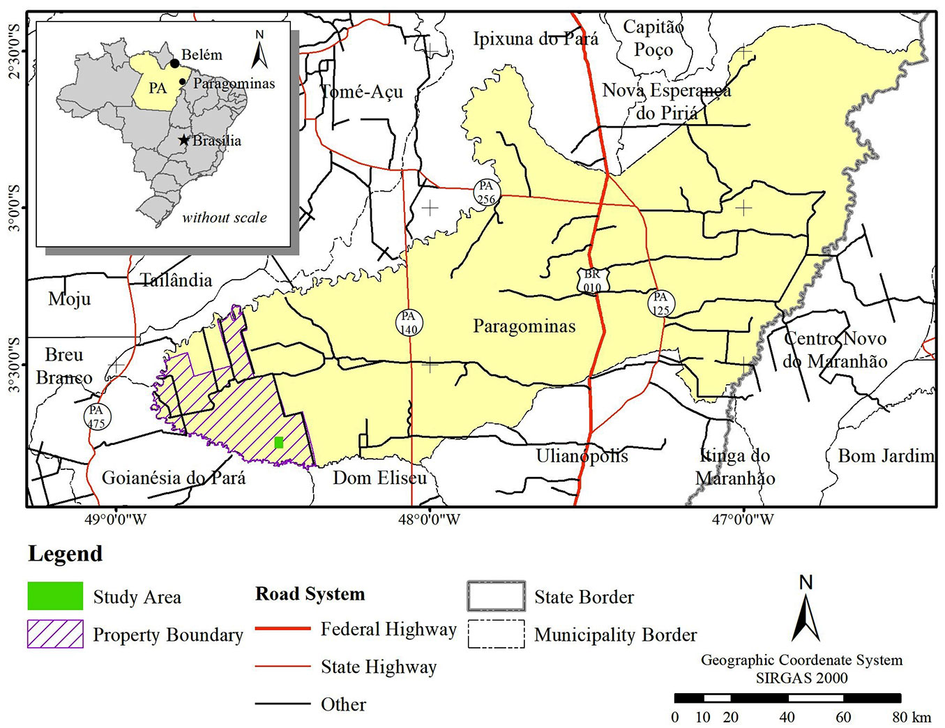
The study area is located at 03° 44′ 59″ South latitude and 48° 28′ 51″ West longitude, in Cauaxi Farm, comprising an area of 1216 ha. The farm belongs to the Rio Capim farm complex, located in the municipality of Paragominas, state of Pará, Brazil, which is part of the Cikel Group domain area (Fig. 1).
Fig. 1 - Location of the study area (Cauaxi farm) in Paragominas, Pará, Brazil. The study area can be accessed via secondary roads (in black), from state highways PA-140 and PA-475.
The Köppen climate classification for the region is “Awi” type, which is tropical rainy with a well-defined dry season. Annual precipitation is around 1800 mm, the average yearly temperature is 26.3 °C, and relative air humidity is 81% ([1]).
The topography of the studied area ranges from flat to gently undulating, and belongs to the Pará-Maranhão Northern Plateau Geomorphological Region ([16]). According to Radambrasil ([43]), the soils are classified as Dystrophic Yellow Latosol.
The dense forest of the high plateau subregion of Pará-Maranhão, the dense floodplain forest, and the terraces characterize the original landscape of the area. Today, it consists of extensive secondary forests characterized by capoeira in various stages of development ([9]).
Ground and LiDAR data acquisition
LiDAR data were obtained from the “Sustainable Landscapes” project of the Brazilian Agricultural Research Corporation (EMBRAPA), which is a technical cooperation project funded by the US Agency for International Development and the US Department of State, and involves the USDA Forest Service and EMBRAPA ([17]) with the aim to generate detailed information on the land surface and vegetation, thus contributing to the measurement of carbon dioxide and other greenhouse gases as well as to the development of mitigation techniques. The project has implemented a WebGIS (⇒ https://www.paisagenslidar.cnptia.embrapa.br/webgis/) that makes available the LiDAR data and the forest inventory database in areas of the Amazon, Cerrado, and Atlantic Forest biomes ([18]).
The forest inventory was conducted in 2014 by establishing 22 plots of 20 × 500 m, comprising an area of 10.000 m2 each and totaling 22 ha. Trees with a diameter at breast height (DBH) ≥ 35 cm were measured for the DBH and crown radius.
LiDAR data were acquired using an aerial platform at an average flight altitude of 850 m. The covered area was 1216 ha, recorded in 20 scenes composed of a point cloud with X, Y, and Z coordinates. The LiDAR data was already georeferenced, and the datum used was SIRGAS 2000 with the Universal Transverse Mercator Projection System (UTM), spindle 22 South.
Definition of minimum gap area
The minimum area of a canopy gap was defined by adapting the method of Hunter et al. ([22]), as the area occupied by a tree crown after its falling/removal. The mean crown radius of each tree was calculated by averaging the four measures (North, South, East, and West) taken in the forest inventory, and its crown area was derived from the average radius. Areas smaller than one m2 were excluded because they are smaller than the 1 m spatial resolution of the generated raster files.
LiDAR point cloud processing
The point clouds generated by the LiDAR sensor were processed using the FUSION/LDV software ([35]). The lowest point density among the 20 different scenes was taken as the minimum point density. This value was used as a reference to standardize the returned point density across the study area. The subsequent analyses were carried out using the calculated minimum density as the reference value (100%) and by resampling fractions of this point density, namely, 75%, 50%, 25%, 10%, and 2% of the reference value. Each of the above six point cloud densities represents a “trial”, which was labeled with the relative number of return points per square meter (ppm2 - see Results).
The “TreeSeg” tool, which performs canopy segmentation, was applied to carry out the gap segmentation. The height threshold was adjusted to 2 m, as reported by Brokaw ([7]). The cells of the canopy height model (CHM) showing values above this threshold were segmented into a single class, while values lower than the threshold were discarded. Also, the maximum height was set at 2 m, therefore only points below this threshold were segmented. The final product was a raster segmented into canopy and gap areas, which was exported (.asc file) for later analyses.
Identification of gap areas and roads
The raster files resulting from the TreeSeg tool were imported in the software QGIS (⇒ https://www.qgis.org/) to transform the data in TIFF files and enable the geospatial analysis of the rasters. A surrounding rectangle was used to crop the raster files and eliminate spurious cells from the edges.
A similar identifier was assigned to the raster cells belonging to the same gap area identified, thus allowing each clearing to be analyzed separately. The area of each gap was calculated (in m2) and the “area_m2” value was added to the attribute table. Gaps were then classified in three groups based on their extension, following criteria adapted from the literature (Tab. 1): (i) Class 1, small gaps from minimum gap area found (a.min) to 149 m2; (ii) Class 2, medium gaps from 150 to 399 m2; (iii) Class3, large and rare gaps ≥ 400 m2.
Tab. 1 - Classes of gap areas used in this study. (a.min): minimum gap area found.
The roads were identified using the segmented raster analysis, with no area classification. The different return point densities used to identify the gaps were analyzed to determine the road layout below the canopy. The visual analysis of the segmented areas allowed to manually design the road paths on the raster, which were then transformed to vectors. Different shapefiles were created for each point density data (= trial) to assess the segments’ length. In addition, the DTM generated from LiDAR data was used to identify the position and the possible layout of watercourses.
Statistical analysis
As the low density of return points from LiDAR can impair the detection of gaps, we verified possible differences in the detection of gaps using different point densities. The Kolmogorov-Smirnov test was applied to test for departure from normal distribution of the area in the three gap classes described above, while the Bartlett’s test was applied to test for equality of variances across the classes. Finally, the non-parametric Kruskall-Wallis test (α = 0.05) was used to test for differences in the estimates of gap area between the different trials (point cloud densities) analyzed.
All the statistical procedures were performed by developing suitable scripts in R v. 3.5.1 and using the RStudio v. 1.1.453 integrated development environment ([44]).
Results
Definition of the minimum gap area
The mean tree crown area for the study area was 55.40 ± 64.88 m2, indicating considerable variability in the data set (Tab. 2). As extreme values may compromise the comparison of data based on the mean ([37]), the median value of tree crown area distribution (34 m2) was chosen as the minimum gap area (a.min) in further analyses.
Tab. 2 - Descriptive statistics of the tree crown areas based on the average crown radius.
| Statistics | Area (m²) |
|---|---|
| Mean | 55.404 |
| Median | 34.732 |
| Mode | 28.274 |
| Standard deviation | 64.878 |
| Minimum | 1.039 |
| Maximum | 1.069.406 |
| Counts | 2.215 (trees) |
LiDAR point cloud processing
The initial processing of the point clouds in FUSION/LDV using the “Catalog” tool revealed an average return density of 61.38 ppm2 (points per squared meters), while the scene with the lowest average density had 37.55 ppm2. Therefore, the latter value was taken as the reference point density to standardize the return density values throughout the study area. The applied return densities were 37, 28, 18, 9, 4, and 1 ppm2 (100%, 75%, 50%, 25%, 10%, and 2% of the reference density, respectively). Consequently, the trials were labelled as T1D37, T2D28, T3D18, T4D09, T5D04, and T6D01, corresponding to the point densities of 37, 28, 18, 9, 4, and 1 ppm2, respectively (Tab. 3).
Tab. 3 - Descriptive statistics of the gap area detected by different return point density (trials, in columns) by class of gap size (in rows, see also Tab. 1). The last number in the trial label correspond to the point density in ppm2. (A.tot): total area (m²); (A.min): minimum area (m²); (A.max): maximum area (m²); (A.avg): average area (m²); (var): variance; (sd): standard deviation; (N): number of gaps.
| Gap Class | Parameter | Trial (% of the reference point cloud density) | |||||
|---|---|---|---|---|---|---|---|
| T1D37 (100%) |
T2D28 (75%) |
T3D18 (50%) |
T4D09 (25%) |
T5D04 (10%) |
T6D01 (2%) |
||
| Class 1 (34-149 m2) |
A.tot | 9,742.00 | 10,267.00 | 11,738.00 | 10,167.00 | 19,130.00 | 17,379.00 |
| A.min | 34.00 | 34.00 | 34.00 | 34.00 | 34.00 | 34.00 | |
| A.max | 147.00 | 147.00 | 147.00 | 147.00 | 146.00 | 149.00 | |
| A.avg | 62.85 | 63.38 | 62.44 | 63.54 | 61.51 | 63.66 | |
| var | 810.92 | 876.91 | 888.96 | 881.36 | 791.55 | 775.43 | |
| sd | 28.48 | 29.61 | 29.82 | 29.69 | 28.13 | 27.85 | |
| N | 155 | 162 | 188 | 160 | 311 | 273 | |
| Class 2 (150-399 m2) |
A.tot | 9,084.00 | 8,800.00 | 9,063.00 | 8,797.00 | 12,220.00 | 12,046.00 |
| A.min | 151.00 | 153.00 | 151.00 | 153.00 | 151.00 | 150.00 | |
| A.max | 397.00 | 386.00 | 396.00 | 386.00 | 392.00 | 382.00 | |
| A.avg | 232.92 | 231.58 | 232.38 | 231.50 | 244.40 | 231.65 | |
| var | 5,492.44 | 5,013.44 | 4,755.45 | 4,997.28 | 5,477.59 | 3,852.94 | |
| sd | 74.11 | 70.81 | 68.96 | 70.69 | 74.01 | 52.07 | |
| N | 39 | 38 | 39 | 38 | 50 | 52 | |
| Class 3 (≥ 400 m2) |
A.tot | 17,665.00 | 18,213.00 | 18,979.00 | 18,221.00 | 20,939.00 | 12,911.00 |
| A.min | 419.00 | 403.00 | 414.00 | 403.00 | 405.00 | 401.00 | |
| A.max | 3,391.00 | 3.398.00 | 3.802.00 | 3.399.00 | 3.708.00 | 3,297.00 | |
| A.avg | 929.74 | 910.65 | 948.95 | 910.55 | 1.046.95 | 860.73 | |
| var | 496.073.90 | 485,124.70 | 598,175.70 | 485,133.10 | 587,919.00 | 542,360.10 | |
| sd | 704.33 | 696.51 | 773.42 | 696.52 | 766.76 | 736.45 | |
| N | 19 | 20 | 20 | 20 | 20 | 15 | |
| Gaps (ha) | - | 3.65 | 3.73 | 3.98 | 3.72 | 5.23 | 4.23 |
| Canopy (ha) | - | 1,170.35 | 1,170.27 | 1,170.02 | 1,170.28 | 1,168.77 | 1,169.77 |
| Total area (ha) | - | 1,174.00 | 1,174.00 | 1,174.00 | 1,174.00 | 1,174.00 | 1,174.00 |
Gap area identification
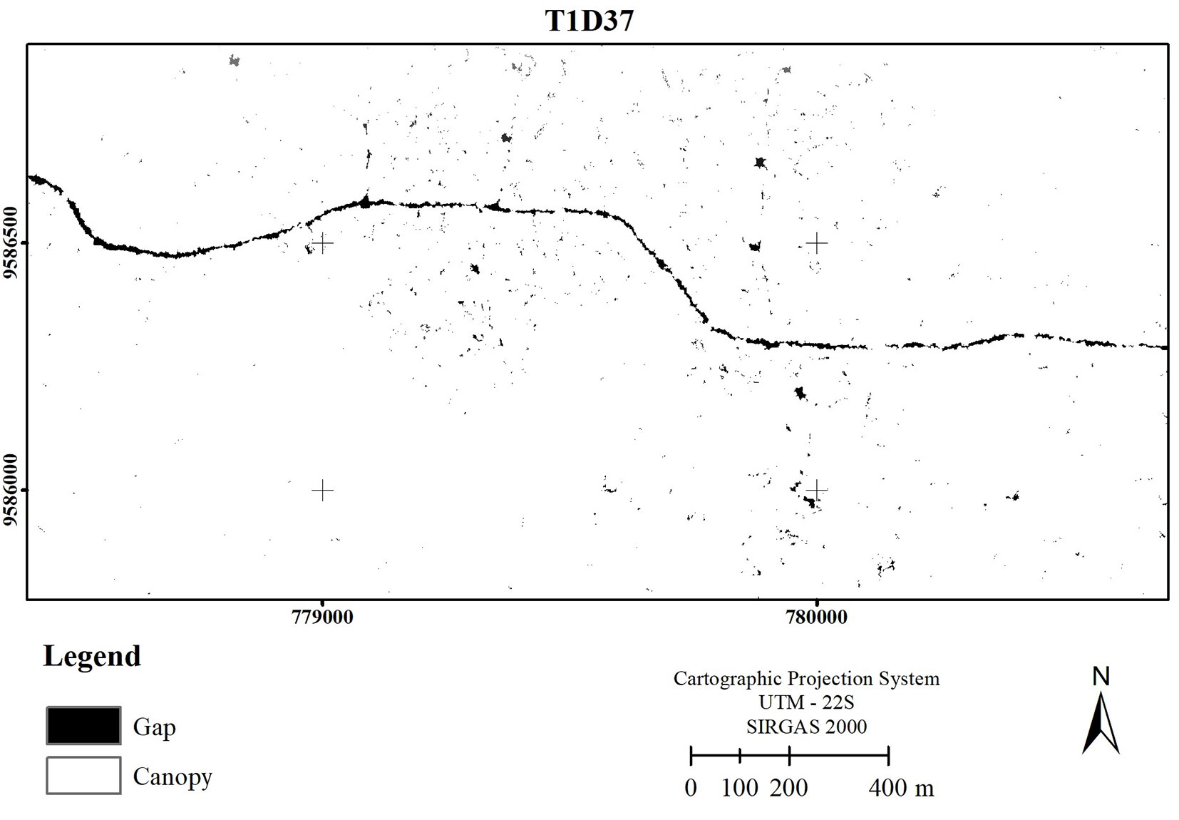
The canopy gaps with area ≥ to 34 m2 (the median value of tree crown areas calculated from the forest inventory) were classified according to the three classes listed in Tab. 1, while smaller areas were not considered as gaps and therefore incorporated into the “Canopy” class (Tab. 3). The pixels of the CHM were grouped according to the height threshold of 2 m; the resulting raster had only two classes (gaps and canopy) and each of the segmented polygons (the canopy gaps) was tagged with its own identifier (Fig. 2).
Fig. 2 - Raster resulting from the segmentation of CHM with clustered pixels for the T1D37 trial. CHM is the canopy height model, and T1D37 is the trial with the highest point density, 37 ppm². Elements in the figure represent gaps (black spots) and canopy (white background).
The result of the Kolmogorov-Smirnov test revealed significant departures (p<0.05) from the normality in the gap area in all classes, meaning that the residues of the three classes did not follow a normal distribution. The homoscedasticity of the data was verified through the Bartlett’s test, which revealed that the variances are homogeneous across the three classes of gap size (p>0.05). The results for both tests are reported in Tab. 4.
Tab. 4 - Results of the normality and homoscedasticity tests. (D): Kolmogorov-Smirnov statistics; (χ2): Chi-square test.
| Class | Kolmogorov-Smirnov | Bartlett | ||
|---|---|---|---|---|
| D | p-value | χ2 | p-value | |
| Class 1 | 0.1581 | 2.2e-16 | 1.9812 | 0.8517 |
| Class 2 | 0.13271 | 0.0002427 | 1.9507 | 0.8559 |
| Class 3 | 0.26658 | 1.837e-7 | 0.42698 | 0.9946 |
A non-parametric test was adopted to evaluate if there was a significant difference between the trials used; thus, the Kruskal-Wallis test was applied. The test results are in Tab. 5.
Tab. 5 - Kruskal-Wallis test result. (χ2): Chi-square test.
| Class | χ2 | p-value |
|---|---|---|
| Class 1 | 2.1751 | 0.8244 |
| Class 2 | 1.4967 | 0.9135 |
| Class 3 | 3.2096 | 0.6677 |
The results of the non-parametric Kruskall-Wallis test (Tab. 5) indicate that there were no significant difference in the between trials (p > 0.05) in any of the three gap area classes. This indicate that any of the six trials (point cloud densities) could be used to identify gaps in the rainforest canopy based on LiDAR sensor data without impairing the gap area estimation.
Road identification
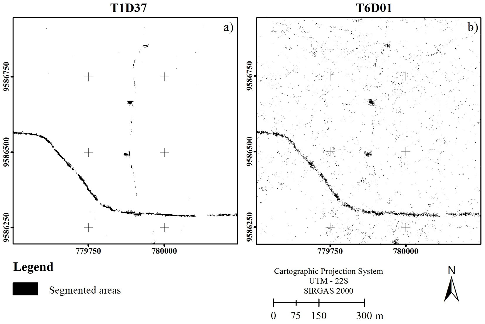
The roads were analyzed qualitatively as they could be identified on the raster resulting from the segmentation. As the return point densities decreased, so did the ability to identify segments that suggested a road layout. Only the main roads could be determined at the lowest point cloud densities, making difficult to detect their presence below the forest canopy. From T3D18 (18 ppm2, i.e., 50% of the reference point density) to the lower-density trials, defining an apparent road layout became more and more challenging, as many segments became discontinuous and because many segments with small areas were generated at lower return densities. Fig. 3shows the segmentation difference in the T1D37 trial with the highest point cloud density and the T6D01 trial with the lowest point clouddensity.
Fig. 3 - Segmentation of road areas in T1D37 and T6D01 trials. The segmented areas represent the roads detected in the exact location with two trials. (a) Trial with the highest density of points, 37 ppm². (b) Trial with the lowest density of points, 1 ppm².
Discussion
To our best knowledge, this is the first study to test the influence of LiDAR return point density on identifying gaps in the Amazon forest. The results evidenced the identification viability by adopting a pre-defined minimum gap area, where the smallest class of gap area had the highest frequency. Based on the results of this study, we reject the hypothesis that there would be a significant difference in identifying forest gaps using different return point densities from LiDAR data in the study area.
The minimum gap area found was similar to that defined by Blackburn et al. ([6]) of 30 m2 in Southern England in a deciduous broadleaved temperate forest. Similar values (35 m2) are reported by Martins et al. ([32]) in the mesophytic semi-deciduous forest in Southeastern Brazil, and by Tabarelli & Mantovani ([48]) in the Atlantic Forest in Serra do Mar, Brazil (30.3 m2). Therefore, both these studies corroborate the minimum gap area found in our study.
Using all trials, the highest number of gaps was found in Class 1 (smaller gaps, 34 to 149 m2). Similar findings were also found by Martins & Rodrigues ([31]) and Martins et al. ([32]) in a mesophytic semi-deciduous forest in Southeastern Brazil, where most of the gaps had area less than 100 m2. Dalagnol et al. ([13]) also found predominantly small gaps (5 to 25 m2), namely 55.3% of 724 gaps. It is worth noting that the different trials (i.e., different point cloud densities) allowed the detection of different gap numbers and areas within the same class, and these differences decreased as the gap area increased (Tab. 3), especially in the number of gaps identified.
In Class 2 (medium gap size), trials T1D37 (100% of the reference point cloud) and T3D18 (50%) allowed the detection of 39 gaps in the forest canopy of the study area, whereas trials T2D28 (75%) and T4D09 (25%) allowed identifying 38 gaps, a difference of only one gap; meanwhile, trials T5D04 (10% of the reference point cloud) and T6D01 (2%) allowed the detection of a larger number of gaps, 50 and 52, respectively. In Class 3 (larger or rare gaps), there was a substantial similarity between trials regarding gap counting, as 20 gaps were identified using trials T2D28, T3D18, T4D09, and T5D04. In the same class, one less gap was identified using the T1D37 trial, while the T6D01 trial allowed to detect 15 gaps.
Regarding the gap area estimates, our results suggest that smaller gaps have more influence on the total gap area at the study site. Indeed, considering Class 2 and Class 3 only, the total gap area was estimated in 2.67 ha using trial T1D37 and 2.70 ha using T2D28 and T4D09. In comparison, T3D18 and T5D04 allowed to estimate larger areas (2.80 ha and 3.32 ha, respectively), while using T6D01 a smaller total area of 2.50 ha was obtained. In a study by Brokaw ([8]) using field measurement methods in the tropical forest in Panama, gaps with areas between 20 and 705 m2 were found. In Martins & Rodrigues ([31]), forest canopy gaps measured with hemispheric photographs (fish-eye lens) in the mesophytic semi-deciduous forest in Southeast Brazil, varied between 20 and 468 m2. The above findings suggest that estimating gap areas from LiDAR data could lead to results consistent with those obtained using traditional methods.
It is important to highlight that the analysis of gap areas carried out in this study evaluated whether there is a significant difference in the size of gaps detected and by size class, not in the total area detected. Indeed, the number of forest canopy gaps detected varied, which could change the total area, but the size of the gaps did not vary.
Using LiDAR detection in a mixed boreal forest in Quebec, Canada, St-Onge & Vepakomma ([46]) found an average gap area of 79.4 m2, and the largest detected areas reached 1743, 1721, and 798 m2. Their findings suggest LiDAR technology as an excellent tool for mapping gaps using a return density of 3 ppm2, which is similar to the point density of the T5D04 trial (4 ppm²) in this study. Treitz et al. ([49]) carried out a plot-level study with different pulse densities, finding that the reduction in density did not reduce the precision of the prediction of forest inventory variables. Similarly, a survey by Jakubowski et al. ([23]) indicated that a high pulse density is not necessary to predict metrics of forest structures at plot level (pixel of approximately 24 m). However, high density is required at the level of individual trees, including the accuracy of tree species identification ([25]) since, according to the authors, the accuracy of metrics decreased as point density decreased.
Using T1D37 trial, a more restricted segmentation in the study area was observed, allowing the detection of a trace following a same direction below the forest canopy (Fig. 3). Using the T6D01 trial, the segmented areas became more diffuse, hampering the identification of the road layout in the raster. Similarly, other free spaces between the tree crowns could lead to the misidentification of forest roads running beneath the canopy, especially using the lower point densities.
Research addressing the detection of forest roads under forest canopy has already been carried out. For example, Azizi et al. ([5]) conducted a study to determine the suitability of LiDAR for forest road detection and extraction, showing that the characteristics of roads obtained using LiDAR data were highly accurate. Similarly, Matinnia et al. ([34]) extracted accurate road longitudinal sections through DTM generated from LiDAR data. The low-density LiDAR data is suitable for detecting and digitizing forest roads over large areas, especially those where forest roads are wide (> 4 m) and are not surrounded by broadleaved stands ([42]).
Regarding point density, Kiss et al. ([26]) evaluated the conditions of forest roads in terms of structural and surface conditions using high point cloud density. The results of a survey conducted by Matinnia et al. ([33]) indicated that the geometric properties of existing forest roads could be monitored under dense forest canopy using LiDAR data.
Airborne LiDAR is widely applied to forests, but its use in the detection of roads and unpaved forest roads is relatively new ([26]). To this end, this study could represent the starting point for more complex methods of road detection, such as developing algorithms for their automatic identification.
The main limitation of this study is the lack of validation of the results based on field data. This is due to the fact that data were not obtained by the authors but from a research project ([17]). Moreover, the issue of the minimum gap area was overcome by adapting a method available in the literature, based on the crown radii measured in the forest inventory. Nonetheless, the main goal of this study was to test whether the reduction in point density of LiDAR data would compromise the detection of gaps, using as a reference the density of the point cloud obtained without degradation of point density.
Conclusions
The reduction in the LiDAR return point density did not affect the detection of gap areas in a tropical forest canopy, rejecting the starting hypothesis of this study. LiDAR data acquisition with a low pulse density, which affect the return point density, seems a feasible option that reduce acquisition costs and improve processing performance. However, the reduction in return densities hampers the detection of roads running underneath the forest canopy. Therefore, the return density reduction for road layout assessment is not recommended in the study area.
LiDAR technology has proven to be an efficient tool for identifying gaps in the forest canopy. It has huge potential for monitoring and planning sustainable forest exploitation. Similarly, it can be applied to monitoring deforestation and illegal logging in tropical forests.
Acknowledgments
The authors thank the Brazilian Agricultural Research Company (EMBRAPA) for providing the data of this study and the Coordination for the Improvement of Higher Level Personnel (CAPES) for financial support (grant no. 1703355).
Conflict of interest
The authors declare no conflict of interest.
Author contribution
JASF: conceptualization, methodology, investigation, formal analysis, writing - original draft; MSS: methodology, data curation, validation; JM: data curation, writing - review and editing; EA: writing - review & editing; RSP: supervision, validation.
References
Gscholar
Gscholar
Gscholar
Gscholar
Gscholar
CrossRef | Gscholar
Gscholar
Online | Gscholar
Online | Gscholar
CrossRef | Gscholar
CrossRef | Gscholar
Gscholar
CrossRef | Gscholar
Gscholar
CrossRef | Gscholar
Gscholar
Gscholar
Gscholar
Gscholar
Authors’ Info
Authors’ Affiliation
Postgraduate Program in Forest Sciences, Federal University of Paraná /UFPR, Lothário Meissner Avenue, 632, Jardim Botnico, 80210-170, Curitiba, PR (Brazil)
Juliana Marchesan 0000-0002-2167-5862
Postgraduate Program in Forest Engineering, Federal University of Santa Maria/UFSM, Roraima Avenue, 1000, Camobi, 97105-900, Santa Maria, RS (Brazil)
Academic Unity of Serra Talhada, Federal Rural University of Pernambuco/UFRPE, Gregório Ferraz Nogueira Av., 56909-535, Serra Talhada, PE (Brazil)
Rural Engineering Department, Federal University of Santa Maria/UFSM, Roraima Avenue, 1000, Camobi, 97105-900, Santa Maria, RS (Brazil)
Corresponding author
Paper Info
Citation
Spiazzi Favarin JA, Sabadi Schuh M, Marchesan J, Alba E, Soares Pereira R (2024). Identification and characterization of gaps and roads in the Amazon rainforest with LiDAR data. iForest 17: 229-235. - doi: 10.3832/ifor4295-017
Academic Editor
Matteo Garbarino
Paper history
Received: Dec 27, 2022
Accepted: Jun 11, 2024
First online: Aug 03, 2024
Publication Date: Aug 31, 2024
Publication Time: 1.77 months
Copyright Information
© SISEF - The Italian Society of Silviculture and Forest Ecology 2024
Open Access
This article is distributed under the terms of the Creative Commons Attribution-Non Commercial 4.0 International (https://creativecommons.org/licenses/by-nc/4.0/), which permits unrestricted use, distribution, and reproduction in any medium, provided you give appropriate credit to the original author(s) and the source, provide a link to the Creative Commons license, and indicate if changes were made.

Web Metrics
Breakdown by View Type
Article Usage
Total Article Views: 15548
(from publication date up to now)
Breakdown by View Type
HTML Page Views: 10235
Abstract Page Views: 2884
PDF Downloads: 2029
Citation/Reference Downloads: 1
XML Downloads: 399
Web Metrics
Days since publication: 684
Overall contacts: 15548
Avg. contacts per week: 159.12
Article Citations
Article citations are based on data periodically collected from the Clarivate Web of Science web site
(last update: Mar 2025)
(No citations were found up to date. Please come back later)
Publication Metrics
by Dimensions ©
Articles citing this article
List of the papers citing this article based on CrossRef Cited-by.
Related Contents
iForest Similar Articles
Review Papers
Accuracy of determining specific parameters of the urban forest using remote sensing
vol. 12, pp. 498-510 (online: 02 December 2019)
Review Papers
Remote sensing of selective logging in tropical forests: current state and future directions
vol. 13, pp. 286-300 (online: 10 July 2020)
Review Papers
Remote sensing-supported vegetation parameters for regional climate models: a brief review
vol. 3, pp. 98-101 (online: 15 July 2010)
Research Articles
Three-dimensional forest stand height map production utilizing airborne laser scanning dense point clouds and precise quality evaluation
vol. 10, pp. 491-497 (online: 12 April 2017)
Research Articles
Integrating area-based and individual tree detection approaches for estimating tree volume in plantation inventory using aerial image and airborne laser scanning data
vol. 10, pp. 296-302 (online: 15 December 2016)
Technical Reports
Detecting tree water deficit by very low altitude remote sensing
vol. 10, pp. 215-219 (online: 11 February 2017)
Technical Reports
Remote sensing of american maple in alluvial forests: a case study in an island complex of the Loire valley (France)
vol. 13, pp. 409-416 (online: 16 September 2020)
Research Articles
Comparing image-based point clouds and airborne laser scanning data for estimating forest heights
vol. 10, pp. 273-280 (online: 23 February 2017)
Review Papers
Remote sensing support for post fire forest management
vol. 1, pp. 6-12 (online: 28 February 2008)
Research Articles
Assessing water quality by remote sensing in small lakes: the case study of Monticchio lakes in southern Italy
vol. 2, pp. 154-161 (online: 30 July 2009)
iForest Database Search
Search By Author
Search By Keyword
Google Scholar Search
Citing Articles
Search By Author
Search By Keywords
PubMed Search
Search By Author
Search By Keyword


