Below- and above-ground biomass, structure and patterns in ancient lowland coppices
iForest - Biogeosciences and Forestry, Volume 10, Issue 1, Pages 23-31 (2016)
doi: https://doi.org/10.3832/ifor1839-009
Published: Nov 06, 2016 - Copyright © 2016 SISEF
Research Articles
Collection/Special Issue: IUFRO division 8.02 - Mendel University Brno (Czech Republic) 2015
Coppice forests: past, present and future
Guest Editors: Tomas Vrska, Renzo Motta, Alex Mosseler
Abstract
Ancient coppice woods are areas that reflect long-term human influence and contain high species biodiversity. In this type of forest we aimed to: (i) analyze the below- and above ground biomass of stools and estimate the age of largest stool; (ii) define a “zone of interference” for coppices; (iii) describe and classify variability in the shape and size of coppice stools; (iv) define the specific characteristics of the spatial distribution of stems and stools. The study was conducted in the Podyjí National Park, Czech Republic, where two old oak coppice stands were fully stem mapped: Lipina (3.90 ha) and Šobes (2.37 ha). Cores were processed using TimeTable and PAST4. Below- and above-ground biomass of the largest stools was computed using the data from terrestrial laser scanner. Tree zones of influence were analyzed with V-Late landscape analysis tools using Shape Index. The pair correlation function and L function were used to describe the spatial patterns of trees with DBH ≥ 7 cm, and the null model of Complete Spatial Randomness and Matérn cluster process were tested. For a modeled old stool, we estimated a ratio of 2:1 for above/below ground volume with no reduction of below ground biomass regarding the hollow roots. The age of the largest stool was estimated 825 ± 145 (SE) years. An “Inner Zone of Influence” was defined, with a total area covering 323 m2 ha-1. The median area of this zone in both plots was 0.40 m2 for all trees, 0.23 m2 for singles and 0.87 m2 for stools. The Matérn cluster process was successfully fitted to our empirical data. In this model, the mean cluster radius ranged between 1.9 to 2.1 m and mean number of points per cluster was 1.7 and 1.9. The most prevalent characteristics of these ancient oak coppices were their compact shape and clustered spatial distribution up to 10 m.
Keywords
Oak, Stools, Spatial Patterns, Root System, Terrestrial Laser Scanning, Ancient Coppices
Introduction
Ancient coppice woods are a specific type of habitat, reflecting long-term human influence and containing high species biodiversity. They conserve local tree ecotypes, and at some sites are the only remnants of original woods with natural species composition, even if the structure of the stands has been modified ([37]). Coppices demonstrate a vast variability and adaptability in the tree and herb layers and in their processes as a whole ([34], [46], [37], [42]). Coppicing is considered to be one of the most important ways to manage temperate lowland (oak-dominated) or highland (beech-dominated) woodlands of West and Central Europe, Eastern Asia and North-East America in reserves or urban areas where this kind of management was historically used ([24], [37], [33], [20]).
For coppice or coppice with standards systems, the most common tree species have traditionally been oaks (Quercus sp.), chestnut (Castanea sativa), lindens (Tilia sp.), hornbeam (Carpinus betulus), and beech (Fagus sylvatica), though others have been used as well ([37]). The main tree species in lowlands is sessile oak Quercus petraea (Matt.) Liebl, a slower-growing but long-lived deciduous tree species whose wood, bark, acorns and litter have versatile uses. Sessile oak can tolerate a considerable lack of moisture and rocky substrates. Late to leaf, this species is associated with spring geophytes, and natural oak or oak-hornbeam woods are generally considered to host light-demanding species of flora and fauna ([13]).
For the purposes of this paper, one or more stems of the same origin creating a single interconnected system were considered as one “tree”. Individual stems were designated as “singles”, while multi-stemmed trees as “stools”. Stools are formed by clonal stems forming interconnected groups or clusters of individuals that originated through vegetative propagation, such as layering, root suckers, stolons or stump shoots, from the same parent plant ([26], [23]).
What distinguishes coppiced trees from trees of seed origin is the root and stool system, which can be very old, crooked and extremely large ([34], [4]). A single coppice stool can have stems several meters away from each other, which nevertheless can be visually identified in the field by experienced observers due to curvatures at the stem bases ([10]) or the typical concentric or linear formations of stems. The age of a stool may be estimated from its diameter; the largest stools are thought to have been continuously coppiced for centuries ([35]).
Since the mid 19th century, continuous coppicing and the ageing of coppice stools have been blamed for lower stand productivity and quality throughout Europe, and especially for the worsening of soil conditions ([48]). However, recent scientific research has not confirmed previous assumptions and has even concluded that in coppice systems, compared to high forests, the decomposition rate and transport of nutrients is faster and soil chemical conditions more favorable, argued to be the consequence of higher light and heat consumption ([19], [7]).
Wu et al. ([51]) introduced the term “ecological field theory” based on the interactions and interferences among plants. Graded circular zones surrounding individual plants (“influence domain” - [49] or “zone of influence” - [50]) were defined. For herbaceous plants, even a Generalized Linear Model concerning the belowground zone of influence has been drawn. This showed that belowground zones of influence are not of fixed circular shapes ([8]). The aim of this paper is to describe and define zones of interference for new seedling recruitment in the case of coppiced trees. Such zones are undoubtedly different from those around trees of seed origin, and for coppiced trees the belowground part is of outstanding importance. We hypothesized that large coppice stools influence the interference potential to a high degree, which a newly germinated seedling would have to overcome to establish itself and successfully grow at a site within the area of a stool.
To describe spatial patterns of stools we used the method of spatial point process analysis, in which the “points” are tree locations and the “marks” tree characteristics such as species, diameter, height, social status etc. ([43]). Due to vegetative reproduction, coppice stands tend to be characterized by high clumping intensities at small spatial scales, i.e., clustered formations. The size and shape of the stool cluster could therefore also be characteristic for different tree species or ecotope conditions, such as terrain exposition, and they play a significant role in determining the age of the stool, in other words the length of continuous human activity - coppicing. Therefore, we also attempted to better define the specific characteristics of the stems and stools in ancient coppices.
To better understanding the structure and patterns in ancient coppices both below and above ground, we asked the following questions: (i) what is the ratio of below- and above-ground structure and biomass of ancient Central European coppices and how old are the largest stools? (ii) What is size of “zone of interference” for coppices - the area around every tree (stool) that is practically inaccessible for natural seed regeneration? (iii) What is the variability in the shape and size of coppice stools? (iv) What are the specific characteristics of the spatial distribution of stems and stools in ancient coppices?
Material and methods
Study site
We studied long-abandoned, sessile oak (Quercus petraea) dominated ancient coppices in the Podyjí National Park (hereafter PNP), Czech Republic. Average yearly temperature in the PNP is between 8 and 9 °C, and average precipitation 550-600 mm ([45]). In a biogeographical sense, the PNP lies in the transition zone between the Hercynian and Pannonian provinces (the mesophytic and the thermophytic) that, together with the varied morphology of the river valley and the plateaux, creates high species diversity ([9]). The PNP is among the longest settled areas in Central Europe, and has been continuously inhabited since 5-6000 BC ([32]). The forest history in the PNP has been described by Vrška ([47]), and Reiterová & Skorpík ([38]). Woodlands in the PNP were intensively influenced by deforestation, pasture, burning, litter raking, cultivation terraces and coppicing.
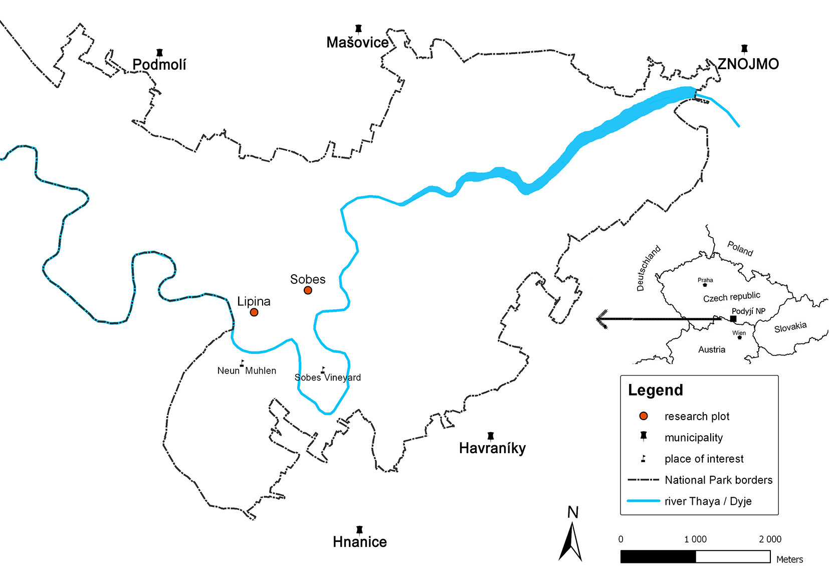
Two research plots, Lipina (3.90 ha - 48° 49′ 19″ N, 15° 57′ 47″ E) and Šobes (2.37 ha - 48° 49′ 32″ N, 15° 58′ 21″ E - Fig. 1), are located in the core (non-intervention) zone of the PNP. Lipina lies on the eastern side of the National Park with an average inclination of 20° and elevation ranging between 300-365 m a.s.l. Šobes lies on the transition ridge between the valley and the plateau, and has more moderate slopes at elevations between 382-395 m a.s.l. The geological bedrock at both sites consists of granites and similar rocks of Proteozoic to Paleozoic age ([38]). The vegetation and soil conditions at Lipina were described in Janík et al. ([21]). The ancient coppices at Lipina, Šobes and other stands in the PNP were left unmanaged after active coppicing started to be abandoned at the end of 19th century and definitively ceased in the 1950s.
Fig. 1 - Location of the research plots within the Podyjí National Park (Czech Republic).
Stool mapping and biomass computation
Tree and stand data were acquired using Field-Map® technology (Jilove u Prahy, Czech Republic), with a MapStar compass module, laser rangefinder, Impulse altimeter (Laser Technology) and Hammerhead field computer (WalkAbout Computers - ⇒ http://www.fieldmap.cz/). All standing and lying trees with diameter at breast height (DBH) ≥ 7 cm and stumps with diameter at the base ≥ 7 cm were measured, and stem position maps were constructed for Lipina in 2006 ([21]) and for Šobes in 2010. For standing stems the following categories were distinguished: live normal, live breakage - snap, full dead stem and snag. Lying deadwood was measured and classified into three stages of decay: hard, touchwood and disintegrated ([25]). For growing shape construction the heights were measured for 10% of standing stems. Height curves were constructed using the Naeslund’s function. During fieldwork in 2010, every standing stem and stump was classified as a single or part of a stool, and the affiliation of stems to stools was recorded in the database using unique IDs for each stool.
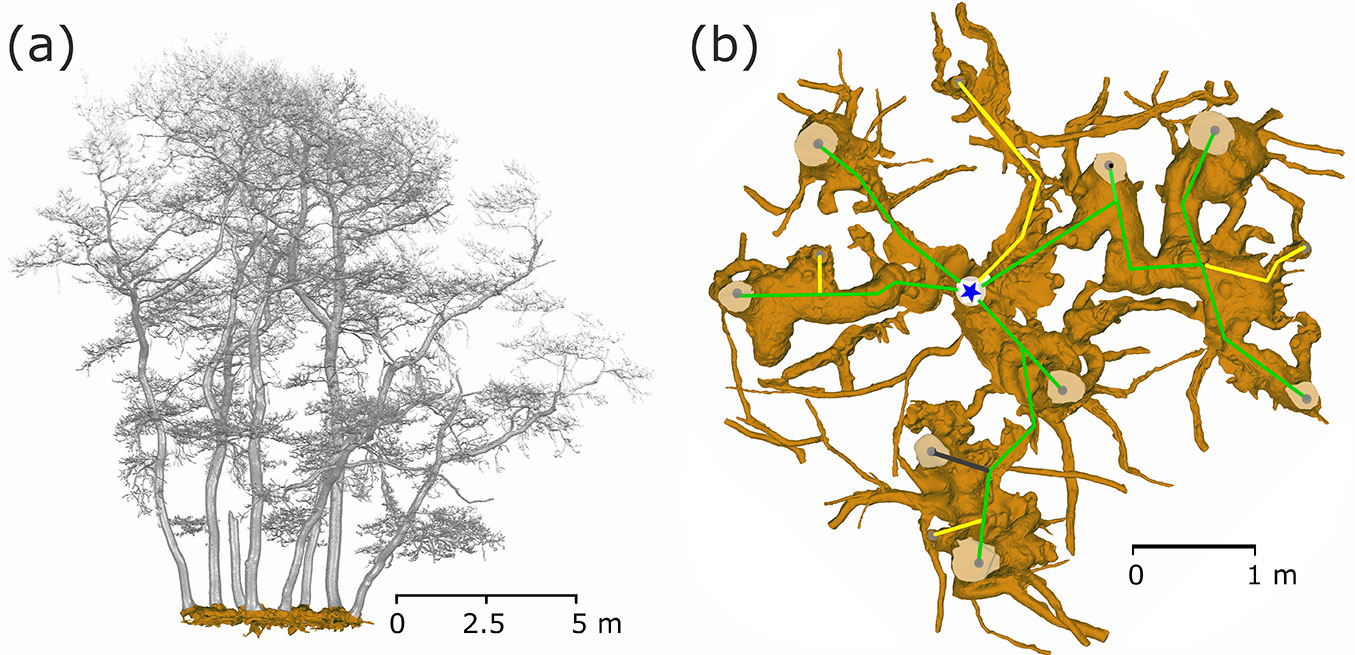
In 2010, we exposed the root systems of three old stools of different sizes and shapes (Fig. 2). Unearthing was performed manually using hand tools, pneumatic drills and an air-spade supersonic nozzle ([31]). We removed the earth to the underlying bedrock at a maximum depth of 65 cm. Exposing the root and stool systems served as a basis for the assessment and mapping of these stools by terrestrial laser scanning. Each uncovered stool was scanned from 9 different positions to record all shapes. After merging all scans into a single one, the resulting point cloud was used to create a model of a stool and its stems (Fig. 2a) for estimating biomass and stem positions. A Leica ScanStation C10™ (Leica Geosystems, Heerbrugg, Switzerland) was used for scanning, together with Cyclone® software for merging single scans, and exported to ASCII file. From the ASCII data, the model of stems, branches and roots was created using Geomagic Studio 2014® software (3D Systems, Rock Hill, SC, USA). A closed manifold surface of all stems and roots that were recognized in stools was generated, and the volume of each part was estimated and a planar projection of each tree and the whole stool was created.
Fig. 2 - Exposed coppice stool root system (Lipina research plot). The current state was captured by a terrestrial laser scanner and saved as a mesh for further analysis. In part (a) the stems are visualized as a side view of the single stool with the whole root system (brown) as a realistic model. A detailed root system model (b) shows all coarse roots, the positions of the living stems (grey dots on stem profiles) and their connections (green - living trees; yellow - historical stumps; grey - standing snags) to the origin (blue star) of the stool.
Stand age analysis and stool age estimation
To survey the age structure of living stems, we sampled the research plots for dendrochronological analysis with an increment borer in 2010. On the basis of stem position maps, we created a regular square network of 44.25 m. At each network point the 2-3 closest live stems were cored. We collected 115 increment cores of individual stems (Lipina: 72; Šobes: 43). The cores were processed using the software packages TimeTable and PAST4 (⇒ http://www. sciem.com/products/past/) with an accuracy of 0.01 mm. To extrapolate the age of cores bored off-pith, missing tree rings were calculated from the measured distance to the estimated pith with a compass and the average width of the first five measured tree rings. Only cores with a maximum of 6 extrapolated tree rings were included into the age analyses (Lipina: 38; Šobes: 26).
For stool age (SA) estimation we used the following formula (eqn. 1):
where AGR is the average growth rate based on annual radial increment, DSR is the average distance of current stems from the parent central root (Fig. 2b), and AAS is the average age of current stems minus 20 as the age used for the AGR. AGR is based on the radial growth of individual stems (shoots), which is simultaneous with the growth of the stool radius; therefore, the growth rate of the entire stool should be twice the radial increment measured on shoots. In practice, the real rate of radius growth of the stool cluster is not twice the mean annual radial growth but is rather somewhat smaller. The reason behind this is that the ground plan projection of the stem circumference is an “inclined plane”. New coppice shoots always spread outwards from the original stump, but because of space restrictions by the original stump, they bend as they grow larger, creating stem curvature at the base and oblique growth. Based on Pigott ([35]), we used a coefficient rate of 1.8 of the mean width increment.
Based on forest management plans from the beginning of the 20th century ([47]), we established that the rotation period at our research plots was intended to be 40 years. Older written material was not so detailed, but previous research has demonstrated that the further one goes back in time, the shorter the coppice cycle tended to be. For instance, in the Middle Ages coppicing was done every seven to ten years ([37]). A twenty-year period was chosen as a long-term average rotation period. According to the historical surveys, the AGR was calculated as the average radial increment of the first 20 tree rings from the dendrochronological analysis of the entire research plot.
DSR was calculated using the 3D model of the stool root and standard image analysis.
Tree inner zone of influence
Fig. 3 - Construction of Tree Area (Tree Inner Zone of Influence) - a projection of individual buffers around the stool and its shape class. Stools were classified by the Shape Index into four classes: circular - single tree (A); circular stool (B); compact polygon(C) and oblong (D).
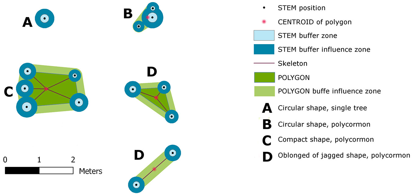
In order to determine the tree interference zone (i.e., the area practically inaccessible for the successful establishment and growth of tree seedlings), we defined the Tree Inner Zone of Influence (TreeIZI). TreeIZI is a closed polygonal area which constituted a projection of (i) the basal area(s) of standing stem(s) or stump(s), (ii) a buffer(s) around the basal area(s), and, in the case of stools, (iii) the stool polygon and (iv) a buffer around the polygon (Fig. 3). The circumference of the stool polygon was created as a link among standing stems or stumps through a procedure of searching nearest neighbors in the stool such that (i) all stems or stumps should lie inside the polygon, and (ii) the circumference line should go directly through each stem or stump position (i.e., a convex hull of stems positions). The buffer size (BS) around each stem or stump was determined by linear scaling according to the diameter (DBH). For smaller trees the buffer radius is a little larger than DBH, while larger trees have a buffer radius almost equal to the DBH value (eqn. 2):
For the circumference, the line of stool buffers with r = the mean diameter of stool was used. Variability analysis and categorization of TreeIZI shapes were carried out with the landscape analysis tool V-Late ([27]) using the Shape Index (eqn. 3):
where Pij is the the perimeter of patch ij in terms of the number of cell surfaces and min Pij is the minimum perimeter of patch ij in terms of the number of cell surfaces. The Shape Index (SI) is a dimensionless expression of compactness. Maximum compactness is represented by a circle; with increasing complexity, crookedness or jaggedness SI also increases. The range of SI is ≥ 1, and is without limit. The V-Late ArcGIS® extension is an implementation of procedures based on Fragstat ([30]).
Tree spatial patterns
To describe the density variability of both individual standing stems and stumps, we used the univariate pair correlation function. The pair correlation function is a second order characteristic, as are the frequently used K function ([39]) and L function ([6]). Stoyan & Penttinen ([43]) define the pair correlation function as follows: consider two infinitesimally small discs of areas dx and dy at distance r. Let p(r) denote the probability that each disc contains a point of the process. Then p(r) = λ 2 g(r) dx dy, where λ is density. Put in a different way, the pair correlation function g(r) is the probability of observing a pair of points separated by a distance r, divided by the corresponding probability for a Poisson process ([1]). It is related to the K function by (eqn. 4):
The essential difference between the K function and the pair correlation function is the non-cumulative character of the latter. The pair correlation function uses annuli as distance classes, not circles. Under the assumption of a homogenous Poisson process, g(r) = 1. Values of g(r) larger than one indicate clustering, while values smaller than one indicate regularity. The pair correlation function g(r) was estimated for each plot at steps of 1 m for r-values up to 20 m. A null model of complete spatial randomness (hereafter CSR) was used on the assumption that the first-order intensity λ is constant within plots. For the fixed value of r we used 199 Monte Carlo simulations of CSR to obtain pointwise critical envelopes for g(r). The significance level of tests was 0.01. A fixed r had to be chosen prior to the simulation, since if all r values are considered simultaneously, the probability of rejecting H0 increases and the true error probability is larger ([29]). Therefore, if we had estimated continuous intervals of the distances over which an observed pattern deviates from the hypothesized model, the results could not have been considered significant with a significance level of 0.01.
A cluster process model was also fitted to the data as an alternative to the Poisson homogenous process. We used the Matérn cluster process, in which the parent points come from a homogeneous Poisson process with intensity κ, and each parent has a Poisson number (μ) of offsprings, independently and uniformly distributed in a disc of radius R centered on the parent ([1]). We used the L function as summary statistics for fitting the model to the data. To determine the values of the parameters that achieve the best match between the fitted LΘ(r) and the empirical L-function of the data, we used the method of minimum contrast ([14]). Since maps of individual plant locations cannot be used to investigate processes occurring at scales that approach the accuracy of the measurements ([15]), and our spatial error was ± 1.1 m, we focused primarily on large-scale processes, such as clustering. All spatial analyses were conducted using the package “spatstat’’ ([2]) in the statistical software R ([36]).
Results
Below- and above-ground biomass and coppice stand structure
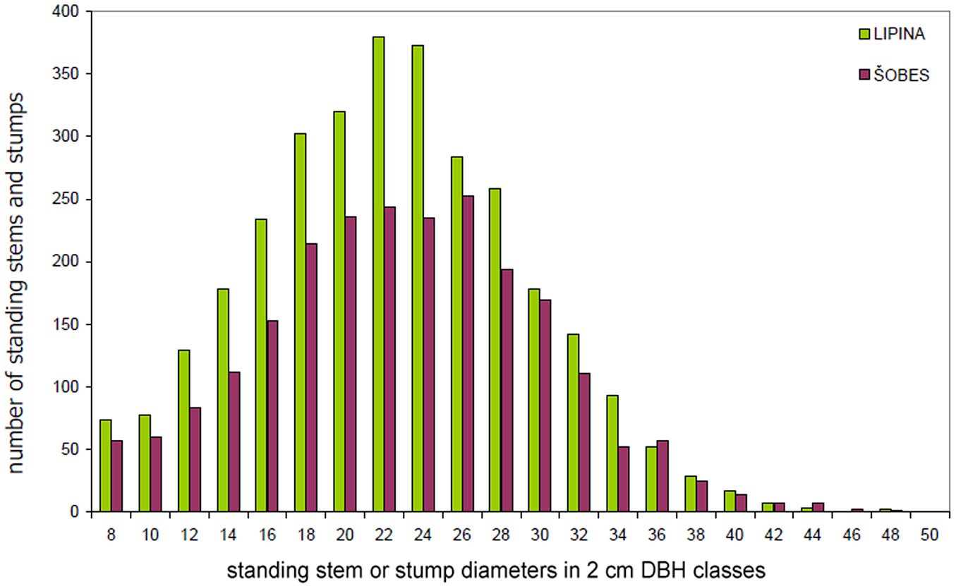
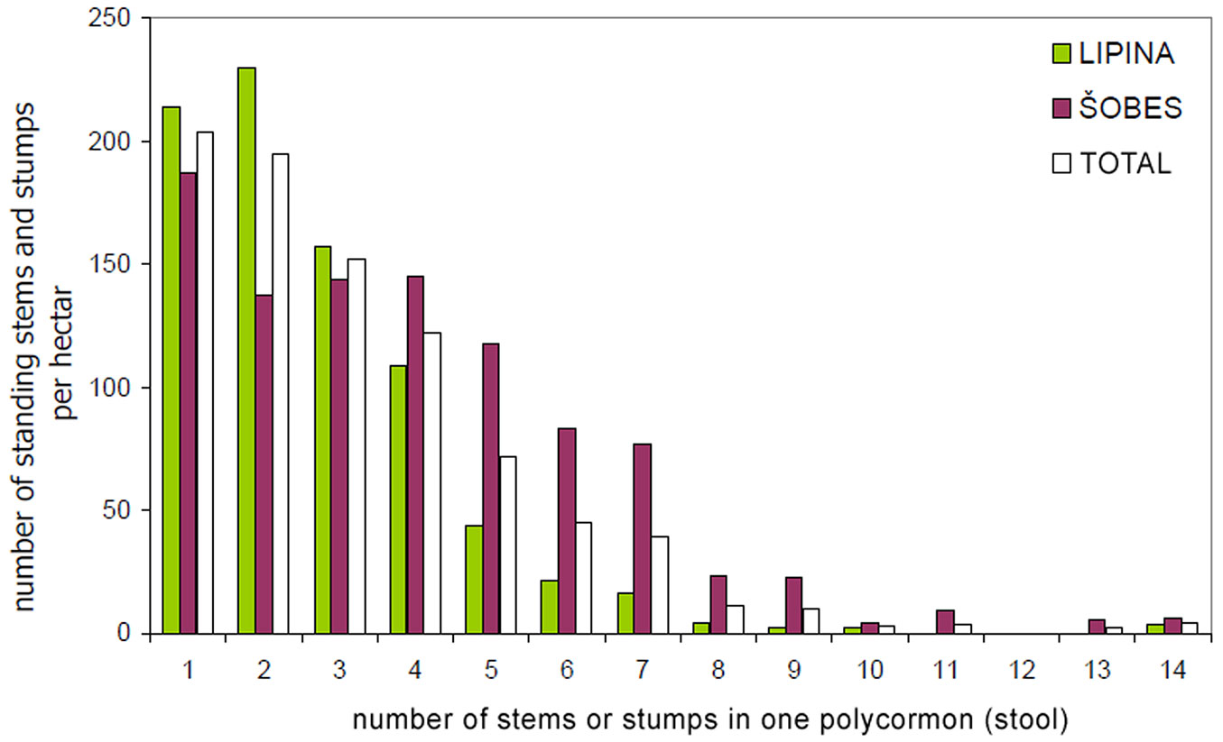
The basic characteristics of the tree layer at Lipina and Šobes are shown in Tab. 1. Approximately 640 live standing stems per hectare represented a timber stock of about 260 m3 ha-1 and a basal area of ca. 30 m2 ha-1. The number of stumps (mostly of artificial origin) was 41 ha-1 at Lipina and 271 ha-1 at Šobes. The median diameter of stems and stumps was 22 cm at both plots, but at Šobes there were more thick individuals (Fig. 4). Long-term coppicing significantly altered the forest structure and texture. The majority of stems and stumps were growing in stools; in total, only ca. 25% were single-stemmed trees (Tab. 2). At Šobes there were proportionally more multi-stemmed trees (stools with 4 and more stems or stumps), but two- and three-stemmed stools still predominated (Fig. 5).
Tab. 1 - Main tree layer parameters at Lipina and Šobes.
| Layer | Parameter | Decay stage | Units | Šobes | Lipina |
|---|---|---|---|---|---|
| - | area | - | ha | 2.37 | 3.90 |
| Live Standing Trees | |||||
| stem no. | - | N ha-1 | 634 | 642 | |
| basal area | - | m2 ha-1 | 32.0 | 29.6 | |
| timber volume | - | m3 ha-1 | 262.0 | 263.0 | |
| Dead Standing Trees | |||||
| stem no. | - | N ha-1 | 59 | 121 | |
| basal area | - | m2 ha-1 | 1.3 | 2.6 | |
| timber volume | - | m3 ha-1 | 7.6 | 16.7 | |
| Stumps | stem no. | - | N ha-1 | 271 | 41 |
| basal area | - | m2 ha-1 | 8.8 | 1.1 | |
| Dead lying stems | stem no. | H | N ha-1 | 16 | 47 |
| T | N ha-1 | 32 | 245 | ||
| D | N ha-1 | 1 | 12 | ||
| Total | N ha-1 | 49 | 304 | ||
| timber volume | H | m3 ha-1 | 2.5 | 12.0 | |
| T | m3 ha-1 | 4.6 | 43.0 | ||
| D | m3 ha-1 | 0.1 | 1.0 | ||
| Total | m3 ha-1 | 7.2 | 56.0 |
Fig. 4 - Diameter distribution of standing stems and stumps at Lipina and Šobes.
Tab. 2 - Numbers and densities of single and multi-stemmed trees (stools), and coverage of the Tree Inner Zone of influence.
| Group | Parameter | Units | Šobes | Lipina | Total |
|---|---|---|---|---|---|
| - | Plot Area | ha | 2.4 | 3.9 | 6.3 |
| Standing single stems and stumps | stools | N | 1841 | 2298 | 4139 |
| N ha-1 | 777 | 589 | 660 | ||
| singles | N | 444 | 834 | 1278 | |
| N ha-1 | 187 | 214 | 204 | ||
| total | N | 2285 | 3132 | 5417 | |
| N ha-1 | 964 | 803 | 864 | ||
| Trees (tree zone of inner influence) |
stools | N | 496 | 820 | 1316 |
| m2 | 768 | 940 | 1708 | ||
| m2 ha-1 | 324 | 241 | 272 | ||
| singles | N | 444 | 834 | 1278 | |
| m2 | 116 | 199 | 315 | ||
| m2 ha-1 | 49 | 51 | 50 | ||
| total | N | 940 | 1654 | 2594 | |
| m2 | 884 | 1139 | 2023 | ||
| N ha-1 | 397 | 424 | 414 | ||
| m2 ha-1 | 373 | 292 | 323 |
Fig. 5 - Frequency distribution of the number of stems or stumps in one stool.
The average upper height of the stand was about 18 meters at both plots. A distinctive difference between the plots was found for deadwood volume, which was more than 4 times higher at Lipina than at Šobes (73 and 15 m3 ha-1, respectively). The dynamics of changes in the tree layer was more pronounced at Lipina, while at Šobes larger gaps in the crown canopy were missing because of the smaller number of fallen dead trees, which were also less disintegrated than at Lipina.
From the modeled stool, above and below ground biomass was calculated. The below ground biomass of the stool was estimated to be 1.02 m3 of woody biomass connecting 7 living stems and one snag, and the sum of the above ground biomass was about 2.13 m3. The stool had a planar projection area of 122.35 m2 with an average stem planar projection area of 26.4 m2. The uncovered area and the root system had an area of about 20 m2.
Stand age and stool age
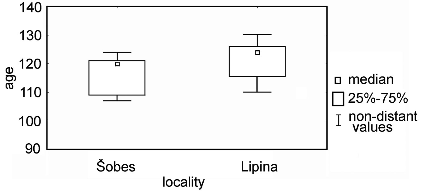
According to the dendrochronological analyses, forest stands at the research plots were last coppiced in 1885 (Lipina) and 1890 (Šobes). The measured mean stem age was 124 years at Lipina (Q25-75: 116-126 yrs) and 120 years at Šobes (Q25-75: 109-122 yrs - Fig. 6). Spot felling could be traced during the Great depression, World War II, and sporadically since the 1950s. During the 1980s/90s, Šobes was thinned as part of a planned transformation into high forest, and the number of stems in one stool was partially reduced. We also detected small-scale thinning at Lipina; stumps from these thinnings can still be easily recognized in the forest, and almost none has re-sprouted with new shoots.
Fig. 6 - Box plot of age distributions at the Lipina and Šobes sites.
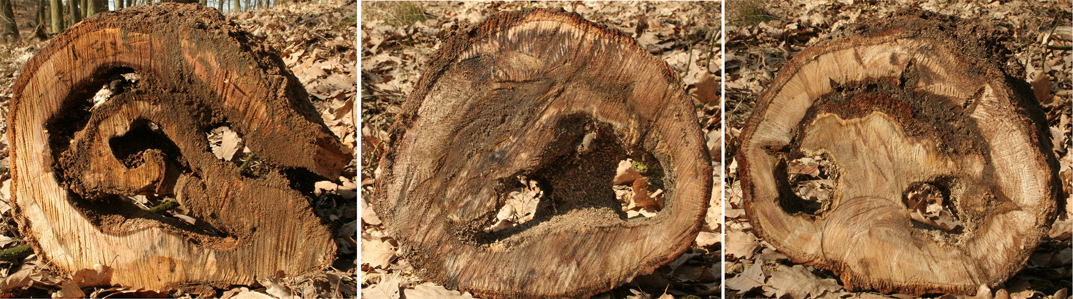
The largest stool (Fig. 2b) had an average distance of 2.13 ± 0.3 m (SE) and an average annual radial increment of 1.46 ± 0.06 mm. The age of this stool was 825 ± 145 years, which means that the stool originated in the 11th-13th centuries (High Middle Ages). Older roots were often hollow inside and we observed a secondary growth of cambium into this hollow space (Fig. 7). This obviously rules out any age analysis.
Fig. 7 - Stool root profile - internal cambium created in the root cavity.
Tree inner zone of influence
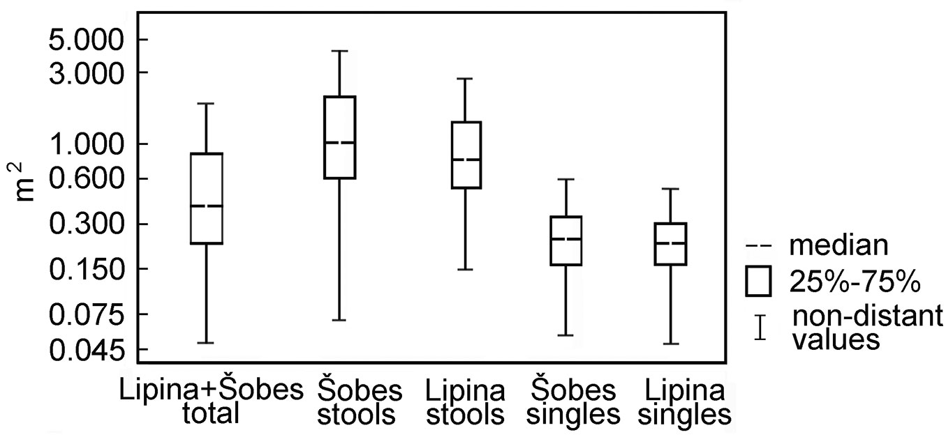
Tree Inner Zone of Influence (TreeIZI) area covered 292 m2 ha-1 at Lipina and 372 m2 ha-1 at Šobes (mean: 323 m2 ha-1). The median area of TreeIZI for a full set of both plots was 0.40 m2 for all trees, 0.23 m2 for singles and 0.87 m2 for stools. At Šobes the Interquartile Range of TreeIZI values was wider compared with Lipina (Fig. 8), and the occurrence of larger stools ≈ larger TreeIZI was more frequent. While the distribution of stem and stump diameters tended to be normal or normal related, the distribution of TreeIZI area was strongly positively skewed and best fit with extreme values or lognormal distribution - even if very few large stools composed a relatively large total of the TreeIZI area.
Fig. 8 - Total tree area (Tree Inner Zone of Influence) for single trees and trees in stools. The box plots show the range of area for single trees and stools in the study plot.
For a basic differentiation of the variety of TreeIZI areas, we used the Shape Index (SI). Based on the results, we defined three categories of TreeIZI shapes: (I) rounded; (II) compact; (III) jagged (Tab. 3, Fig. 3), by comparing to the boundary values of SI for the basic, mathematically easily definable shapes of a pentagon (SI = 1.075) and equilateral triangle (SI = 1.285). Both in numbers and area, the most prevalent was category II (compact - Tab. 3). Mean patch size at Lipina was smaller than at Šobes for all categories, most significantly in category III (jagged). In general, for our data raising SI raises the patch size of TreeIZI (Pearson’s r = 0.4856; significance of F for regression analysis: p<0.0001).
Tab. 3 - Shape types and tree types according to the Shape Index, along with basic characteristics of the Tree Inner Zones of Influence. (NP): number of patches; (MPS): mean patch size; (PSSD): PS standard deviation; (MSI): mean shape index.
| Class | Shape type | Tree type |
Criterion | NP (N ha-1) |
Class Area (m2 ha-1) |
MPS (m2) |
PSSD | MSI | |||||
|---|---|---|---|---|---|---|---|---|---|---|---|---|---|
| Šobes | Lipina | Šobes | Lipina | Šobes | Lipina | Šobes | Lipina | Šobes | Lipina | ||||
| I | circular | single | SI ≤ 1.001 | 187 | 214 | 49 | 51 | 0.26 | 0.24 | 0.12 | 0.11 | 1.001 | 1.001 |
| I | circular | stool | SI ≤ 1.075 | 13 | 10 | 10 | 5 | 0.82 | 0.46 | 0.98 | 0.18 | 1.054 | 1.038 |
| II | compact | stool | 1.075 < SI ≤ 1.285 | 167 | 149 | 251 | 174 | 1.5 | 1.17 | 1.18 | 0.97 | 1.171 | 1.186 |
| III | elongated or jagged | stool | SI > 1.285 | 29 | 52 | 62 | 62 | 2.14 | 1.2 | 2.21 | 1.31 | 1.367 | 1.363 |
| Total | - | - | - | 396 | 424 | 372 | 292 | - | - | - | - | - | - |
Tree spatial patterns
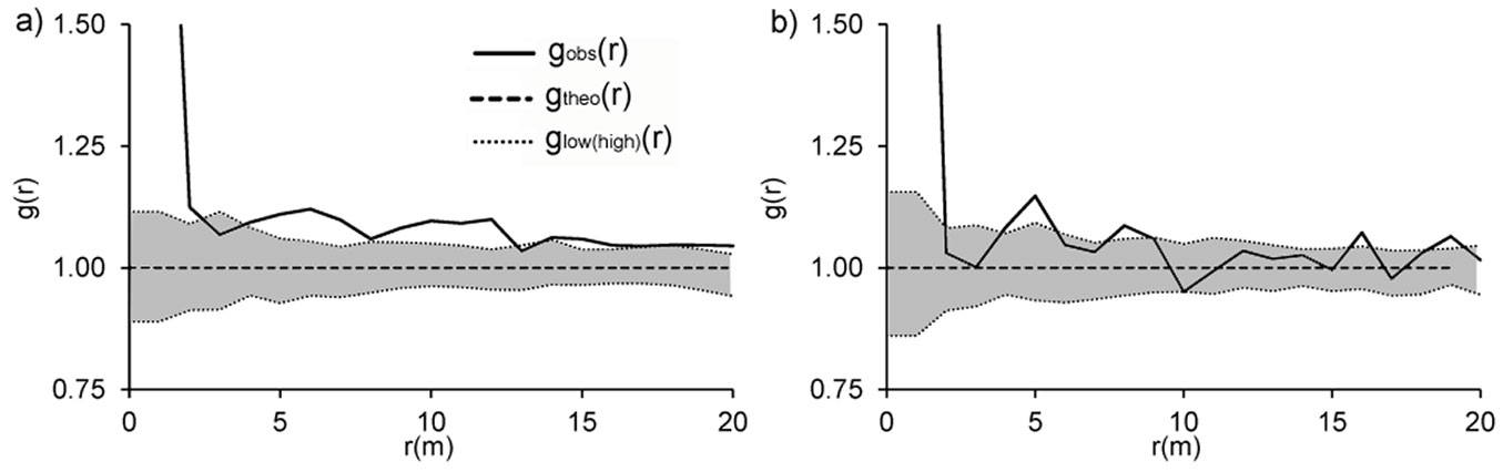
Our evaluation of the spatial distribution of all standing stems and stumps (both singles and stools) resulted in slight differences between the two plots (Fig. 9). While at Lipina stems and stumps were significantly clustered over all examined distances (Fig. 9a), at Šobes for the majority of distances complete spatial randomness (CSR) could not be rejected, and a significantly clustered distribution was confirmed only for individual distances (1, 4, 5, 8, 16 and 19 m - Fig. 9b). Since the CSR hypothesis was rejected for the distribution of trees at Lipina and partly at Šobes, the Matérn cluster process was fitted to our empirical data. The minimum contrast method based on the L function yielded the estimates R = 2.11 m (cluster radius), c = 1.85 (mean number of points per cluster) and intensity κ = 0.04 m-2 for Lipina stems and R = 1.22 m, c = 1.68 and κ = 0.05 m-2 for stems at Šobes. The empirical L function and envelopes from 199 simulations of the fitted model showed good agreement for Šobes trees in particular.
Fig. 9 - Pair correlation functions g(r) show spatial patterns of all stems at Lipina (a) and Šobes (b). gobs(r): observed function; gtheo(r): theoretical value for complete spatial randomness; glow(high)(r): pointwise envelopes resulting from 199 Monte Carlo simulations of the null model of complete spatial randomness. When gobs(r) > ghigh(r), a positive association between stems is suggested, while gobs(r) < glow(r) suggests a negative association of stems. In the grey zone, the null hypothesis of complete spatial randomness cannot be rejected. The variable “r” refers to distance.
Discussion
Ancient stool roots and age
Because roots are generally less accessible and more difficult to explore and measure, they are less well known than the aboveground parts of plants. A detailed morphological and anatomic analysis of root systems can potentially indicate relationships between roots, the outside environment and other organisms at a particular site. The analysis of root systems, especially in the case of older individuals, can be used to gain insights into the complex and long-term driving factors influencing individual stands. The analysis of roots of oak on skeletal soils have shown that in such conditions trees sometimes develops distorted plates or slats, which are pushed into the small spaces between rocks or fissures of the parent rock ([22], [42]). Oak tree rings are visible only in root ends and adjacent areas of surface skeletal roots, which also show other signs of transitional anatomy between aboveground and underground organs ([22], [5]). As a result, dendrochronological cores of old roots cannot be used to determine the age of ancient coppice stools.
Structural differences in wood anatomy are more variable for broadleaf trees than for conifers ([16]), making it much more difficult to detect changes in the wood in response to various events. Because the influences of climate, stand density, and social position of a tree causes large variability in ring width pattern, Copini et al. ([11]) rejected to use the patterns of wide rings around the pith, previously utilized by Haneca et al. ([17], [18]) as a fingerprint of coppice management. Our findings are in agreement with these views.
To examine the age of ancient stools and the processes that led to their current shape, one must go beneath the surface to uncover the root and stump system. We made a visual and acoustic evaluation (by tapping on roots) of the exposed underground of ancient stools and took cross sections of different roots. We concluded that the overwhelming majority of large roots were hollow because of heart rot or were preserved only as remnants of the original root in the form of slab roots. Because the oldest parts of the roots were decayed, the deadwood samples we were able to take could not serve as indicators of stool age. The approximated age of one of the largest oak stools at our research plots was 825 ± 145 years (SE). Similar or even older coppice stools of oaks and lindens with respect to size and growth rate have been reported by Rackham ([37]) and Pigott ([35]).
For the modeled old stool we estimated a ratio of 2:1 for above/below ground volume with no reduction of below ground biomass regarding the hollow roots. This is in contrast to Barbaroux et al. ([3]), who found a 5:1 biomass estimation ratio in a high forest. Stem bases were clustered only at 20 m2 but the trees were spread into the neighbourhood and altogether covered a 5 times greater area than in high forest.
Tree inner zone of influence
In our study we simplified the shape of stool clusters into three categories: (I): rounded; (II): compact; (III) jagged. However, the number of variants can be very high depending on tree species: coppicing ability and strength, mortality rate and its spatial distribution, length of rotation period, longevity and rate of growth.
The present form of ancient coppices was shaped by the mortality of new shoots due to mutual competition, the ageing and dying of old stools ([28], [41]), as well as by natural habitat conditions and the length, intensity and frequency of human impact. The probability of sprouting steeply declines for stools with large DBH. If many sprouts persist on a single stump, they may develop a sweep in the lower part of the bole.
It appears that for most oak species the key factor limiting seedling recruitment is light availability, i.e. overstory crown closure. Seed regeneration is therefore far more likely in open sites away from the parent tree ([12], [13]). However, with the gradual decay and dying off of ancient oak stools, one can expect an increase in seedlings of tree species other than oak (lime, hornbeam, maple, pine - [44]).
Tree spatial patterns
In accordance with our assumptions, stems often showed a significantly clustered distribution. This reflects the vegetative origin of stems in stools. At Lipina, stems had clustering at all study intervals up to 20 m. A similar spatial distribution was observed in the Mondariz and Pantón coppice forests in Spain ([40]). The maximum intensity of clumping in our study and in Mondariz and Pantón is almost identical, with ranges at ca. 1 m.
Interestingly, stool centroids also showed a clustered distribution at distances to 10 m. This could be the effect of long-term human influence (short-rotation period). If the stems were cut at a young age (7-10, later 20 years), then the forest stand was essentially single-layered at all times. All stems needed a minimal crown area for survival, and less successful trees were gradually eliminated, so the forest stand tended towards a clustered spatial distribution.
Conclusions
For the modeled old stool we estimated a ratio of 2:1 for above/below ground volume with no reduction of below ground biomass regarding the hollow roots. The age of the largest stool was estimated 825 years ± 145 years (SE). Total area of “Inner Zone of Influence” covers 323 m2 ha-1. The median area of this zone in both plots was 0.40 m2 for all trees, 0.23 m2 for singles and 0.87 m2 for stools. The Matérn cluster process was successfully fitted to our empirical data. In this model the mean cluster radius ranged between 1.9 to 2.1 m and mean number of points per cluster was 1.7 and 1.9. The most prevalent characteristics of these ancient oak coppices were their compact shape and clustered spatial distribution up to 10 m.
Acknowledgements
We would like to thank the Podyjí National Park Administration for supporting our research. Ivana Plačková, Dagmar Koktová, Saly Šmíd and Fidel Švejda helped us to unearth the coppice stools. Thanks to Hanuš Vavrčík from the Faculty of Forestry and Wood Technology, Mendel University in Brno for consulting the dendroecology of roots. For comments on the manuscript, we thank to Martin Valtera. David Hardekopf carried out the proofreading. This paper was created with support of projects GA CR P503-11-2301 and OPVK CZ.1.07/2.3. 00/20.0267.
References
Gscholar
Gscholar
Gscholar
Gscholar
Online | Gscholar
Gscholar
Gscholar
Gscholar
Gscholar
Gscholar
Gscholar
Online | Gscholar
Gscholar
Gscholar
Gscholar
Gscholar
Gscholar
Gscholar
Gscholar
Authors’ Info
Authors’ Affiliation
David Janík
Marcela Pálková
Dusan Adam
Jan Trochta
Silva Tarouca Research Institute, Department of Forest Ecology, Lidická 25/27, 602 00 Brno (Czech Republic)
Marcela Pálková
Faculty of Forestry and Wood Technology, Mendel University in Brno, Department of Silviculture, ZemÄ›dÄ›lská 3, 613 00 Brno (Czech Republic)
Corresponding author
Paper Info
Citation
Vrška T, Janík D, Pálková M, Adam D, Trochta J (2016). Below- and above-ground biomass, structure and patterns in ancient lowland coppices. iForest 10: 23-31. - doi: 10.3832/ifor1839-009
Academic Editor
Francesco Ripullone
Paper history
Received: Aug 31, 2015
Accepted: Aug 12, 2016
First online: Nov 06, 2016
Publication Date: Feb 28, 2017
Publication Time: 2.87 months
Copyright Information
© SISEF - The Italian Society of Silviculture and Forest Ecology 2016
Open Access
This article is distributed under the terms of the Creative Commons Attribution-Non Commercial 4.0 International (https://creativecommons.org/licenses/by-nc/4.0/), which permits unrestricted use, distribution, and reproduction in any medium, provided you give appropriate credit to the original author(s) and the source, provide a link to the Creative Commons license, and indicate if changes were made.

Web Metrics
Breakdown by View Type
Article Usage
Total Article Views: 53773
(from publication date up to now)
Breakdown by View Type
HTML Page Views: 44086
Abstract Page Views: 3553
PDF Downloads: 4590
Citation/Reference Downloads: 77
XML Downloads: 1467
Web Metrics
Days since publication: 3528
Overall contacts: 53773
Avg. contacts per week: 106.69
Article Citations
Article citations are based on data periodically collected from the Clarivate Web of Science web site
(last update: Mar 2025)
Total number of cites (since 2017): 17
Average cites per year: 1.89
Publication Metrics
by Dimensions ©
Articles citing this article
List of the papers citing this article based on CrossRef Cited-by.
Related Contents
iForest Similar Articles
Research Articles
Use of terrestrial laser scanning to evaluate the spatial distribution of soil disturbance by skidding operations
vol. 8, pp. 386-393 (online: 08 October 2014)
Research Articles
Three-dimensional forest stand height map production utilizing airborne laser scanning dense point clouds and precise quality evaluation
vol. 10, pp. 491-497 (online: 12 April 2017)
Research Articles
Efficient measurements of basal area in short rotation forests based on terrestrial laser scanning under special consideration of shadowing
vol. 7, pp. 227-232 (online: 10 March 2014)
Research Articles
Predicted occurrence of ancient coppice woodlands in the Czech Republic
vol. 10, pp. 788-795 (online: 16 September 2017)
Research Articles
Are we ready for a National Forest Information System? State of the art of forest maps and airborne laser scanning data availability in Italy
vol. 14, pp. 144-154 (online: 23 March 2021)
Research Articles
Determining basic forest stand characteristics using airborne laser scanning in mixed forest stands of Central Europe
vol. 11, pp. 181-188 (online: 19 February 2018)
Technical Advances
Forest stand height determination from low point density airborne laser scanning data in Roznava Forest enterprise zone (Slovakia)
vol. 6, pp. 48-54 (online: 21 January 2013)
Research Articles
Integrating area-based and individual tree detection approaches for estimating tree volume in plantation inventory using aerial image and airborne laser scanning data
vol. 10, pp. 296-302 (online: 15 December 2016)
Research Articles
Relationship between tree growth and physical dimensions of Fagus sylvatica crowns assessed from terrestrial laser scanning
vol. 8, pp. 735-742 (online: 11 June 2015)
Research Articles
Terrestrial laser scanning as a tool for assessing tree growth
vol. 10, pp. 172-179 (online: 19 November 2016)
iForest Database Search
Search By Author
Search By Keyword
Google Scholar Search
Citing Articles
Search By Author
Search By Keywords
PubMed Search
Search By Author
Search By Keyword


