The potential of using xylarium wood samples for wood density calculations: a comparison of approaches for volume measurement
iForest - Biogeosciences and Forestry, Volume 4, Issue 4, Pages 150-159 (2011)
doi: https://doi.org/10.3832/ifor0575-004
Published: Aug 11, 2011 - Copyright © 2011 SISEF
Research Articles
Abstract
Wood specific gravity (WSG) is an important biometric variable for aboveground biomass calculations in tropical forests. Sampling a sufficient number of trees in remote tropical forests to represent the species and size distribution of a forest to generate information on WSG can be logistically challenging. Several thousands of wood samples exist in xylaria around the world that are easily accessible to researchers. We propose the use of wood samples held in xylaria as a valid and overlooked option. Due to the nature of xylarium samples, determining wood volume to calculate WSG presents several challenges. A description and assessment is provided of five different methods to measure wood sample volume: two solid displacement methods and three liquid displacement methods (hydrostatic methods). Two methods were specifically developed for this paper: the use of laboratory parafilm to wrap the wood samples for the hydrostatic method and two glass microbeads devices for the solid displacement method. We find that the hydrostatic method with samples not wrapped in laboratory parafilm is the most accurate and preferred method. The two methods developed for this study give close agreement with the preferred method (r 2 > 0.95). We show that volume can be estimated accurately for xylarium samples with the proposed methods. Additionally, the WSG for 53 species was measured using the preferred method. Significant differences exist between the WSG means of the measured species and the WSG means in an existing density database. Finally, for 4 genera in our dataset, the genus-level WSG average is representative of the species-level WSG average.
Keywords
Wood specific gravity, Aboveground biomass, Dry xylarium samples, Tropical forests, Congo basin forest
Introduction
Tropical deforestation and degradation are estimated to have released on the order of 1 - 2 Pg C / yr (15 - 35 percent of annual fossil fuel emissions) during the 1990s ([12]). A key technical challenge for the successful implementation of mechanisms that can help reduce emissions from deforestation and degradation is the reliable estimation of the aboveground biomass (AGB) in tropical forests. Reliable estimation of AGB depends on a number of sampling issues, including sampling of spatial variability, determination of forest structural allometry and determination of tree wood density, also known as wood specific gravity (WSG).
WSG is defined as the ratio of the oven-dry mass of a sample to the mass of a volume of water equal to the volume of the sample at a specific moisture content ([1]) and is calculated by dividing the mass of a sample by its volume. Although mass is easy to determine, the volume determination is a less straightforward procedure. Moreover, sampling a sufficient number of trees for WSG to represent the species and size distribution in highly diverse tropical forests is time consuming and costly. For tropical regions, published data on wood specific gravity are frequently limited to a number of commercial timber species that only represent a fraction of the forest biomass.
On the other hand, there are collectively hundreds of thousand wood samples held in xylaria (botanical collection with wood samples from lignified plants ([3]) around the world, spanning wide geographic areas including the tropics and many tens of thousands of species ([31]).
Given the above, this paper focuses on WSG by: (1) exploring the possibility of obtaining the WSG of tropical tree species using xylaria samples; we examined the accuracy and practicality of five different methodologies, two solid displacement methods and three liquid displacement methods (of which two were specifically designed and developed for the purposes of this paper); (2) measuring wood sample volume for the purpose of calculating WSG; and (3) providing a preliminary ecological assessment of WSG for 53 species in the Congo Basin in which we illustrate inter-individual variation in WSG, make a comparison of the WSG values of the species we measured to an existing wood density database, and examine genus-level WSG representativeness for species-level WSG.
Background
There exists a great diversity of tropical woods with densities ranging from 0.1 (“light woods”) to 1.2 (“heavy woods”) g/cm3. WSG is considered as a crucial wood property affecting the properties and value of both solid and fibrous wood products ([24]). As a good predictor of mechanical properties of wood, it is often viewed in relation to support against gravity, snow, wind and other environmental forces ([11]).
Furthermore, WSG is an important factor for AGB estimates ([2], [20], [30]). The most important predictors of ABG of a tree are its trunk diameter, wood specific gravity, total height and forest type ([7]). The most important source of error in AGB estimation is currently related to the choice of allometric model ([7]). However, ignoring variations in WSG can result in mediocre overall prediction of the ABG biomass stand ([2]) greenhouse-gas emissions ([20]).
With regards to forest dynamics, WSG is related to the growth and mortality rates of a tree species ([19]) and provides information on life-history strategies of tree species ([13]). Additionally, WSG is a strong indicator of ecological succession stages with the pioneer species having greater variation and being less dense than climax species ([35], [19]). Several studies have shown that wood density is positively related to drought resistance in tropical trees ([11], [29]) and shrubs ([10]). Given the above, it is indeed unfortunate to find that the wood density of many tropical trees remains unknown ([30]).
As density is one of the most important parameters of wood quality, its measurement methods have been the subject of general publications on the physical properties of wood and moisture relations (cf. [28], [27]) and specific measurement methods papers, such as: medical CAT-scan imaging for very small samples ([16]); stereometric method ([26]); mercury method (cf. [8]); microdensitometer techniques ([6], [25], [18], [5]); basic density (dry weight / wet volume) for freshly collected samples for conversion to AGB ([9]); vibrational spectroscopy such as near infrared reflectance (NIR - [34], [33]), Fourier Transform Infrared (FTIR) spectroscopic bands ([32]) and Diffuse Reflectance Mid-Infrared Fourier transform (DRIFT-MIR - [22]).
The above methods all have several advantages and disadvantages related to them. The main disadvantages related to some of the methods described above are: high cost; inability to take the xylarium samples out of the place they are stored (building); the fact that most samples do not have uniform or regular geometrical shapes; that the cutting of sub-samples is not allowed; and the phasing out of mercury in many industries. What is clear is the need to develop feasible, practical, quick and cheap non-destructive methods to determine the volume of xylarium samples.
Material and methods
The wood sample collection
As a case study, we chose to focus on the major tropical forest region with perhaps the greatest deficit of ecological information: the Congo Basin Forest. The xylarium of the museum for central Africa in Tervuren (Belgium) holds the largest collection of wood samples for the Congo Basin Forest in the world ([4]). Some samples have relatively precise descriptions of the trees (estimated height, large or small tree) and locations from where they were collected. There are also several samples per species, genus and family, making it possible to conduct a detailed study on the across- and within-taxon variability of WSG. The xylarium also holds wood samples of what are now rare and protected species that could be difficult to collect today.
Particularities of using xylarium samples
Due to the long-term mission of the xylarium, samples are dry and have to remain in their original condition, i.e., the structural and chemical state of the sample must be preserved. Determining the WSG of such samples presents several difficulties. First, the format of the samples is not standard (e.g., irregular shapes, small planks, book shaped planks and circular pieces of wood). Second, it may not be allowed to cut pieces off the samples. Third, the samples may not be allowed to be covered in paraffin, wetted or treated with any chemical that may damage the sample, both in appearance and in any physical or molecular way. Last, the samples may perhaps not leave the designated area or be transported elsewhere for further studies.
Terminology
Of all the physical properties of wood, WSG was the first to be examined systematically. An overview of the data from 18th and beginning of 19th century has been given by Chevandier & Wertheim (1848) in Kollmann ([14]). We employ the terminology provided by the American Society for Testing and Materials (ASTM) specific gravity for wood can be defined as the ratio of the oven-dry mass of a sample to the mass of a volume of water equal to the volume of the sample at a specific moisture content ([1]). Given that both the mass and, below the fibre saturation point, volume of wood vary with the amount of moisture contained in the wood, specific gravity as applied to wood is an indefinite quantity unless the conditions under which it is determined are clearly specified. The specific gravity of wood is based on the oven-dry mass, yet the volume may be that in the oven-dry, partially dry or green condition ([1]).
Sample selection and preparation for volume assessment
Two size categories of wood samples were selected: samples under 10 x 10 cm cross-sectional area and samples above 10 x 10 cm (hereafter referred to as “small” and “large” samples, respectively). The samples are of irregular shapes and sizes with varying degrees of surface smoothness. One hundred small samples were selected of 24 different species. For the large samples, 18 samples were selected of 15 different species.
To reach oven-dry mass, samples were dried in an oven for 48 hours: 2 hours at 60 °C, 4 hours at 80 °C and 42 hours at 103 °C to achieve constant weight. Temperature was increased gradually to minimise the risk of cracking the samples. Samples were weighed immediately after being taken out of the oven. The moisture content of the samples held in the xylarium before oven-drying (eqn. 1) was 8 percent. Samples under 2.1 g were weighed to the nearest 0.01 g while samples above 2.1 g were weighed to the nearest 0.1 g due to the limitations of the electronic balances used (eqn. 1):
where m g is the mass of the wood sample as held in the xylarium and m od is the oven dry mass of the sample (attained after the oven drying and reaching constant mass). Volume measurements were done after the samples were oven dried and hence we measured an oven-dry WSG.
Sample selection for ecological assessment
The sample selection for a preliminary ecological assessment focused on the regional scale of the Congo Basin Forest. Some 976 samples from 53 species were measured. Species were selected based on the following criteria: (1) each species needed to have a minimum of ten samples that could be measured; and (2) each species had to occur in more than one region of the Congo Basin forest.
A comparison was made between the species means for the measured species and the means of the same species found in the Global Wood Density Database (GWDD - [36]) using a two-sample t-test assuming unequal variances at a five percent significance level. In order to evaluate whether or not genus-level WSG averages were representative of species-level WSG averages, a nested analysis of variance (ANOVA) was used.
Liquid displacement methods
These are methods based on Archimedes’ principle: the volume of a sample is estimated by the mass of the volume that is displaced while the sample is submerged in liquid. The method used for this study is known as the hydrostatic method. In this method, the mass of the liquid which is displaced by the sample (oven-dry) is determined. A beaker is filled with water and placed on a digital balance. The balance is then re-zeroed. The sample is attached to an adjustable screw clamp (of which the volume is known and corrected for when submerged in the water), which is in turn attached to a vertically moving arm of a stand. The measured weight of displaced water equals the sample’s volume (since water has a density of 1). The electronic balance was re-zeroed after every measurement. Three repetitions were made for each sample with the hydrostatic method. Three variations of the hydrostatic method were tested, using the same principle as described above and the same samples:
- Samples wrapped in laboratory parafilm. The samples were weighed before coating and after coating them in laboratory parafilm. The difference in weight was subtracted from the volume of the sample. The disadvantage with laboratory parafilm wrapping is that it may trap air. Wrapping the wood samples in laboratory parafilm was developed specifically for the purposes of this paper. We used laboratory parafilm “M” which is water repellent and self-adhesive.
- Samples not wrapped in laboratory parafilm. The volume of the sample was taken, the sample was dried off and the following repetition was made. Samples were not re-weighed after each measurement to account for increase in weight.
- Samples not wrapped in laboratory parafilm, with re-weighing the samples after each measurement in order to take account of increase in weight due to water absorption. The sample was weighed, the volume was of the sample was taken, the sample dried off, its weight taken, the difference in weight added to the volume of the sample (accounting for absorption) and the following repetition made.
Solid displacement method
These methods are based on the principle that solid materials are used to measure the volume of a given sample. Two solid displacement methods were tested:
- Sand using a vibrating bed for compaction. For this method calibrated white sand was used. Sand was poured into a glass beaker until reaching a required volume (e.g., 100 ml). The beaker containing the sand was placed on a vibrating bed for 10 seconds to ensure compaction of the sand particles at a predefined volume (e.g., 100 ml). In a second glass beaker recipient, some of the sand was poured in to cover the bottom of the recipient and subsequently the sample was placed on the sand. The rest of the sand was poured on top of the sample until the sand containing the sample reached the same initial volume (100 ml) once again followed by compacting the sand on the vibrating bed. The remaining sand (again compacted) represents the volume of the sample. Two repetitions were made for each sample. A third measurement was taken if the difference between the two volume measurements was above 5 percent.
- Glass microbeads using height drop for compaction. This machine was designed specifically for this study (Fig. 1). The concept of the machine is a semi-closed system of two glass recipients connected by a graduated cylinder (each 2 ml graduation) held in a wooden structure. Two machines were built, one for small samples and one for larger samples. For the small samples, the volume of the graduated cylinder is 100 ml and approximately 95 cm in vertical height. For the large samples, the graduated cylinder is 1000 ml and the vertical height approximately 110 cm. The method works like an hourglass. There is a constant amount of glass microbeads in the glass recipients (of 0.5 micrometers), the volume of which is read off the graduated cylinder (e.g., 20 ml). The system is rotated on its own axis and the glass micro-beads run into the second glass recipient. The sample is placed in the first glass recipient that can be opened. Once the sample is placed in the container, the system is turned around on its axis once more. The volume is once again read ( e.g., 50 ml) and the difference in volume is the volume of the sample ( e.g., in this example the volume equals to 30 ml). Two repetitions were made for each small sample. If the difference was greater than 5 percent, a third repetition was made. Three repetitions were made for the large samples.
Fig. 1 - Glass micro-beads machines using height drop for compaction.
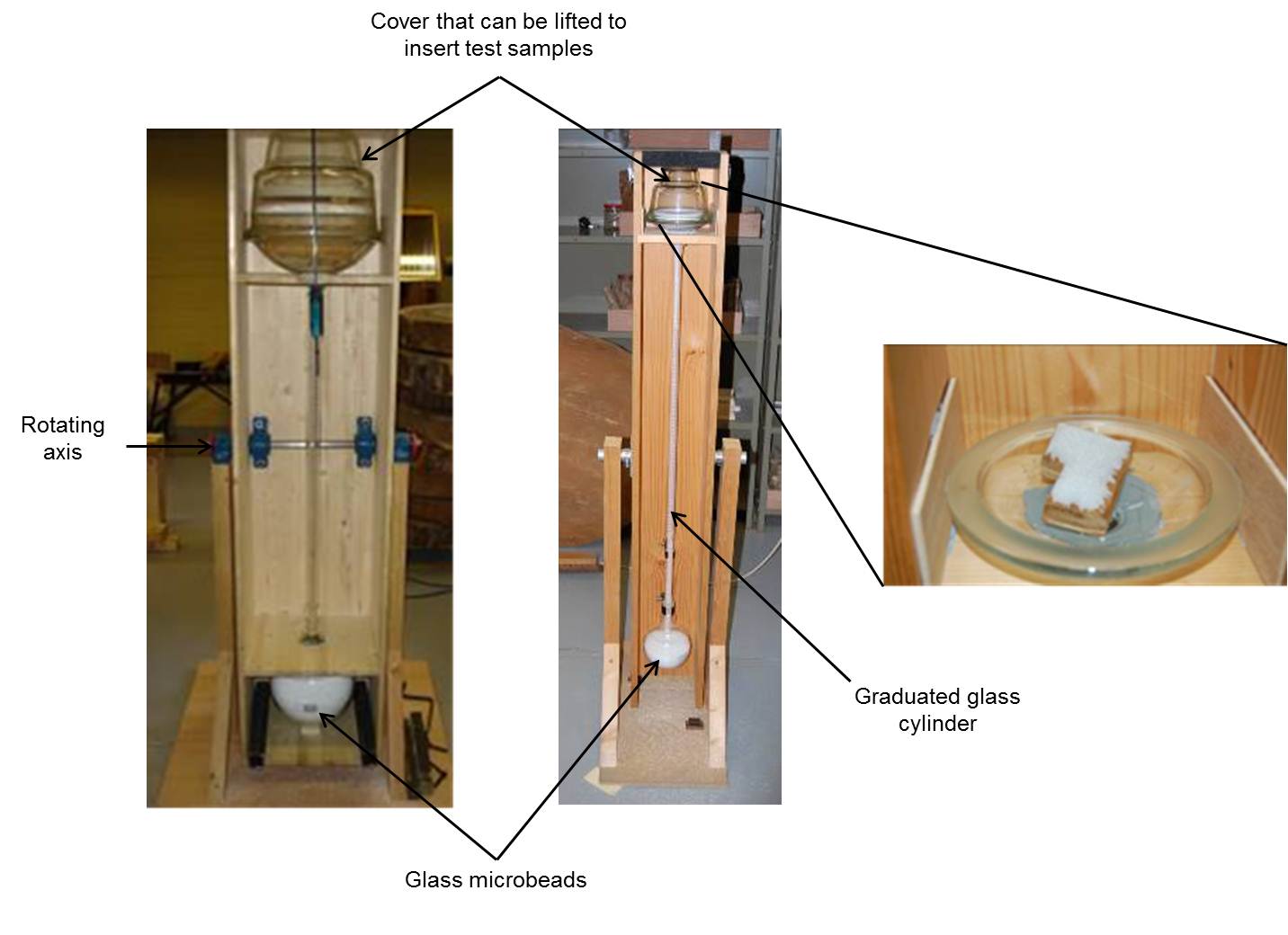
To test the accuracy of the two machines with known volume samples, the Walloon Agricultural Research Centre conducted the volume measurements on 56 different samples. Different defined shapes with smooth surfaces and known volumes were produced and measured using in the devices. For the smaller device, 10 cubic shaped samples (8.1 to 263 cm3), 10 cylindrical shaped samples (3.4 to 279 cm3) and 10 parallelepiped shaped samples (16.7 to 184 cm3) were processed in 5 replications. For the larger device, the 8 cubic shaped samples (126 to 700 cm3), 9 cylindrical shaped samples (30 to 1127 cm3) and 10 parallelepiped shaped samples (91.6 to 310 cm3) were processed in 5 replications.
To evaluate the influence of each tested method on the wood sample density results, individual and global mean values, we calculated mean WSG and two measures of dispersion, the standard deviation and coefficient of variation of the WSG values ([35]). To compare the mean values of WSG obtained by the different methods, ANOVA were conducted at a significance level of 5 percent. A one-way ANOVA procedure was used for pair-wise multiple comparisons. The agreements between the chosen “preferred” method and other methods were evaluated using the coefficient of determination (r 2) and the F-statistical test for bias, slope = 1 and intercept = 0 using SAS software ([17], [15]).
Results and discussion
Tab. 1 shows the mean densities (g/cm3) and density ranges (g/cm3) for the measured wood samples. The sand method was only used for the 100 small samples. It appears to overestimate mean density and the standard deviation is highest. On the other hand, the glass microbeads method appears to underestimate WSG. Besides the case for the 18 large samples, this underestimation is similar to the underestimation when using laboratory parafilm. With the glass microbeads, it might be that the compaction of the beads is insufficient, giving a higher volume for the samples. For the wood samples wrapped in parafilm the increased volume is most likely due to the trapping of air between the sample and the parafilm. The mean densities of the hydrostatic method correcting for absorption and the mean densities of the plain hydrostatic method are very similar. The patterns described can be observed clearly when looking at a randomly chosen samples (Fig. 2).
Tab. 1 - Summary table of mean densities ± SE (g/cm3) and density ranges (g/cm3).
| Method | 100 small samples | 18 large samples | Combination of samples (118) | |||
|---|---|---|---|---|---|---|
| Mean density | Density range | Mean density | Density range | Mean density | Density range | |
| Sand (solid displacement) | 0.79 ± 0.24 | 0.22 1.62 | - | - | - | - |
| Glass micro-beads (solid displacement) | 0.65 ± 0.18 | 0.16 0.98 | 0.62 ± 0.22 | 0.24 1.12 | 0.65 ± 0.18 | 0.16 1.12 |
| Wrapped in laboratory parafilm (hydrostatic) | 0.65 ± 0.17 | 0.17 0.97 | 0.64 ± 0.20 | 0.29 1.04 | 0.65 ± 0.17 | 0.17 1.04 |
| Not wrapped in laboratory parafilm and not correcting for absorption (hydrostatic) |
0.70 ± 0.18 | 0.19 1.04 | 0.69 ± 0.21 | 0.30 1.10 | 0.70 ± 0.19 | 0.19 1.10 |
| Not wrapped in laboratory parafilm but accounting for absorption (hydrostatic) |
0.71 ± 0.19 | 0.19 1.08 | 0.69 ± 0.21 | 0.30 1.11 | 0.70 ± 0.19 | 0.19 1.11 |
Fig. 2 - Wood sample density for 10 small samples and 6 large samples estimated by five different methods. The y-axis shows the wood specific gravity of a sample depending on the method used. Each column on the x-axis represents the WSG values for one sample. The sand method is only used for the small samples. Error bars show the standard deviation. S1 stands for sample 1 and so on.
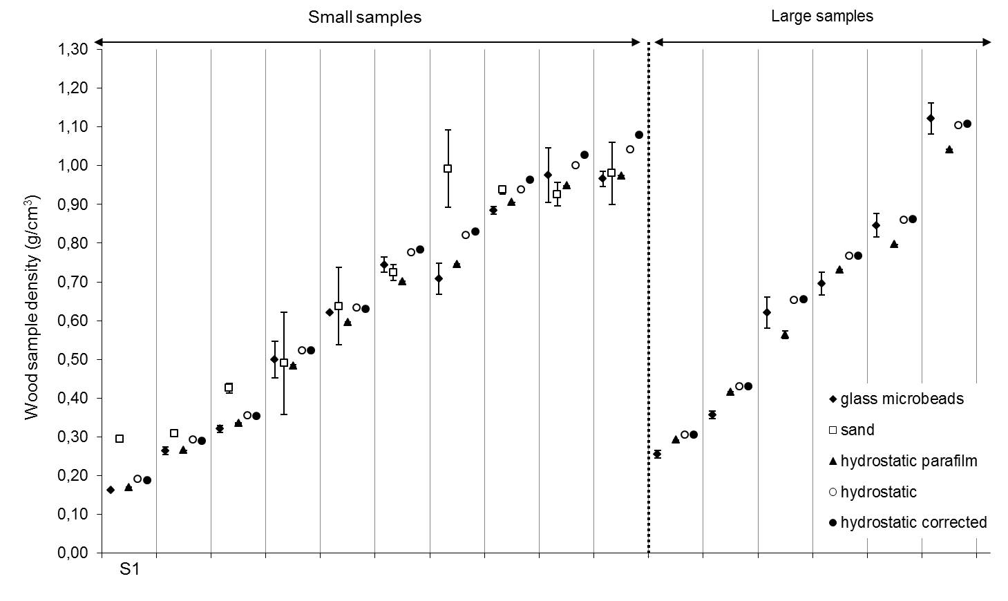
Large standard deviations for the sand and glass microbeads method are observed (Fig. 2: S4, S5, S7, S9, S10, S13, S14, S15 and S16). Assuming that the samples did not fall into the same position within the glass cylinders at each repetition, perhaps the sand particles and glass microbeads could not compact around the sample in the same manner, explaining the larger variation.
We performed an ANOVA on three sets of data: (1) 100 small samples; (2) the 18 large samples; and (3) the small and large samples put together (see below).
- Small samples: the method has a significant effect on the estimation of density (p < 0.01). The Levene statistics test rejects the null hypothesis that the group variances are equal (p >0.05). Using Tamhanes’ test which does not assume equal variances, for the small samples, we find that there is a significant difference between the glass microbeads method and the sand method (p < 0.01), the sand method and the hydrostatic parafilm method (p < 0.01) and between the sand method and the hydrostatic method (p < 0.05);
- Large samples: the choice of method has no significant effect on the mean density (p > 0.05). The Levene statistics test rejects the null hypothesis that the group variances are equal (p > 0.05). Using Tamhanes’ statistic, we find that there is no significant difference between the groups on mean density. Indeed, it appears that the sand method used on the small samples was the most problematic;
- Combined: we find that choice of method has a slight but significant effect on the mean density (p < 0.02). The Levene statistics test rejects the null hypothesis that the group variances are equal (p > 0.05). Using Tamhanes’ statistic, we find that there is no significant difference between the groups on mean density.
Regarding the hydrostatic method for samples not wrapped in parafilm but re-weighing after each measurement (correcting for absorption), there is an increase in volume for the samples when absorption is taken into account. There is an average volume increase of 0.61 percent for small samples and 0.29 percent for large samples. This has an impact of 0.61 percent on the mean density of the small samples and 0.29 percent for the large samples, affecting the mean density by the same amounts. This percentage can be regarded as negligible meaning that either hydrostatic method with samples not wrapped in parafilm could be a “preferred” choice of method. Not wrapping the samples in parafilm but correcting for absorption was chosen as the “preferred” method based on its precision and comprehensive approach for this study. However, this choice should be evaluated for each study and could, for example, be ranked on an assessment of an allowable error for the WSG measurement.
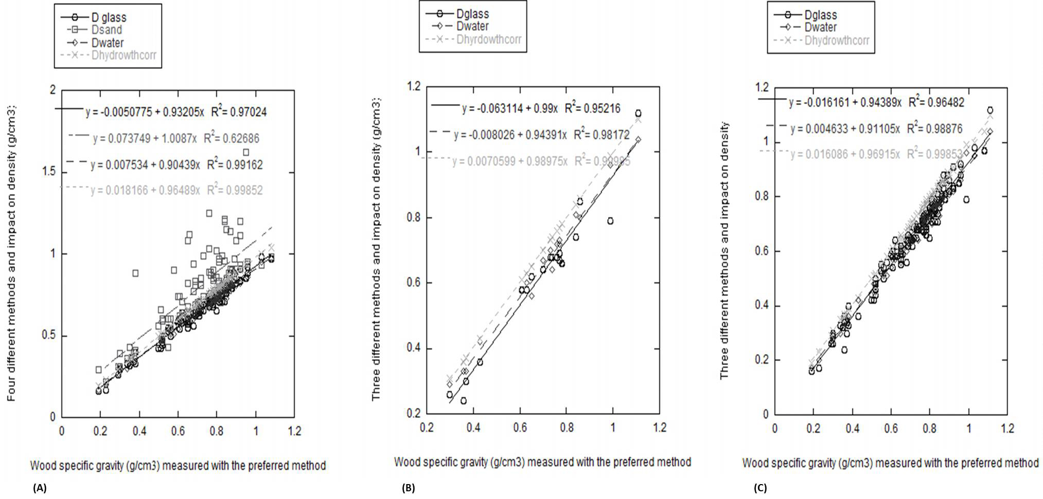
All subsequent regression analyses use the “preferred” method against which the other four methods are tested (Fig. 3 and Tab. 2). The relationships between the preferred method and other methods were satisfactory for all methods excluding the sand method. For the small samples, the large samples and the small and large samples combined, the coefficient of determination for: (a) the hydrostatic method (without parafilm or correction for absorption), (b) the hydrostatic method with parafilm, and (c) the glass microbeads method is highly significant (r 2 > 0.95 in all cases). Hence, any of these three other methods are valid depending on the limitations of the samples to be worked with. However, the simultaneous F-test for bias, slope = 1 and intercept = 0 was significant for all methods and small, large or combined samples (p < 0.001) but one: the 18 large samples not wrapped in laboratory parafilm. The slope was significantly different from 1 for sand - 100 small samples; glass microbeads - 100 small samples; not wrapped in laboratory parafilm - 100 small samples and combined. The intercept was significantly different from 0 for sand; all three categories of samples for glass microbeads; not wrapped in laboratory parafilm - 100 small samples and combined.
Fig. 3 - Regression analyses comparing the “preferred method” (hydrostatic method without parafilm wrapping but with correction to take account of water absorption) to the other different tested methods: (A) for 100 measured small samples, (B) for 18 measured large samples and (C) for all measured samples.
Tab. 2 - Statistical summary of linear regression (F-statistic) of the preferred method against the other methods. Slope H0 = 1, intercept H0 = 0; (*): p < 0.05; (**): p < 0.01; (***): p < 0.001.
| Preferred method | Sand | Glass micro-beads | Wrapped in laboratory parafilm | Not wrapped in laboratory parafilm and not correctingfor absorption | ||||||
|---|---|---|---|---|---|---|---|---|---|---|
| Linear regression | 100 small samples | 100 small samples | 18 large samples | combined | 100 small samples | 18 large samples | combined | 100 small samples | 18 large samples | combined |
| Adjusted R2 | 0.63 | 0.97 | 0.95 | 0.96 | 0.99 | 0.98 | 0.99 | 1 | 1 | 1 |
| Slope | 0.62***± 0.05 | 1.04*± 0.02 | 0.96± 0.05 | 1.02± 0.02 | 1.1***± 0.01 | 1.04± 0.04 | 1.09***± 0.01 | 1.03*** ± 0.0 | 1.0± 0.0 | 1.03*** ± 0.0 |
| Intercept | 0.22***± 0.04 | 0.03*± 0.01 | 0.1*± 0.04 | 0.04***± 0.01 | -0.00± 0.01 | 0.02± 0.02 | 0.0 0.01 | -0.02***± 0.0 | -0.0± 0.0 | -0.01***± 0.0 |
| Bias | 55.35*** | 140.46*** | 19.63*** | 144.82*** | 700.52*** | 21.35*** | 525.06*** | 100.48*** | 2.2 | 77.69*** |
| % under or overestimation | 38% | -4% | 4% | -2% | -10% | -4% | -9% | -3% | (none) | -3% |
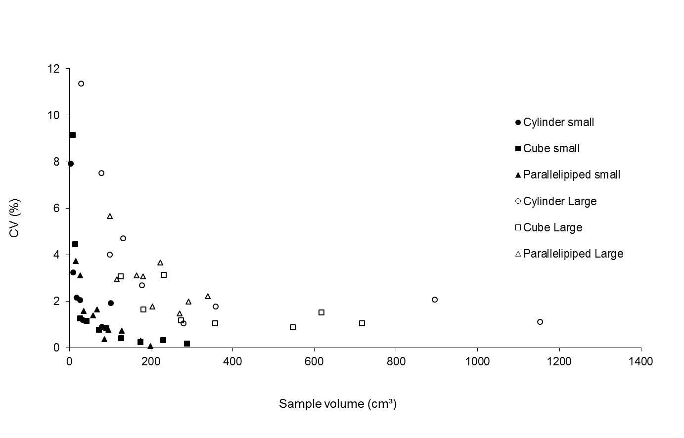
The analysis of the coefficient of variation shows that the shape of the sample did not influence the precision of the method (Fig. 4). On the other hand, it is clear that the coefficient of variation is higher for lower volumes. Moreover, the variation is higher for the larger device, compared to the small one. In order to improve the precision of the method it is advisable (Tab. 3) to avoid the use of small samples. The relative accuracy of the method improved from 2.30 percent (all tested samples) to 1.29 percent (sample volume > 20 cm3) for the small device and from 3.60 percent (all tested samples) to 2.74 percent (sample volume > 100 cm3) for the larger device.
Fig. 4 - Measurements for the coefficient of variation (5 repetitions) for two devices (small and large) as a function of the sample volume.
Tab. 3 - Precision of the different sample sizes and glass microbeads devices used.
| Method | Avg. STD | Avg. CV (%) | Accuracy dr for N = 5 (%) |
|---|---|---|---|
| Small device/All samples | 0.78 | 1.85 | 2.30 |
| Small device / sample volume > 20 cm3 | 0.84 | 1.04 | 1.29 |
| Large device / All samples | 6.00 | 2.90 | 3.60 |
| Large device / Sample volume > 100 cm3 | 6.13 | 2.21 | 2.74 |
Preliminary ecological application
We provide a preliminary ecological assessment of the data collected. The WSG of the samples was measured using the preferred method. Tab. 4 provides a summary of the WSG values for each of the 53 species and compares the measured values to the values found in the GWDD ([36]). For the species where a comparison of the averages could be made between the measured means and the means derived from the GWDD, there exists a significant difference between the means (p < 0.05 - indicated in Tab. 4 with an asterisk).
Tab. 4 - WSG of the measured samples per species compared to the WSG values in the GWDD. WSG values from the GWDD were taken for species occurring in Africa, as the measured species all originate from Central Africa. An asterisk (*) next to a species name indicates a significant difference (p < 0.05) between the mean of the measured values and the mean of that species in the GWDD.
| Species | No. Samples measured | Average WSG ± STD (g/cm3) | Range WSG(g/cm3) | No. values given in GWDD | WSG value GWDD ± STD (g/cm3) | WSG value GWDD range (g/cm3) |
|---|---|---|---|---|---|---|
| Albizia adianthifolia | 15 | 0.56 ± 0.13 | 0.38 - 0.86 | 7 | 0.51 ± 0.06 | 0.45 - 0.65 |
| Albizia gummifera | 19 | 0.57 ± 0.08 | 0.43 - 0.71 | 7 | 0.53 ± 0.06 | 0.47 - 0.65 |
| Alstonia congensis | 12 | 0.35 ± 0.09 | 0.27 - 0.62 | 8 | 0.33 ± 0.03 | 0.29 - 0.39 |
| Autranella congolensis* | 20 | 0.88 ± 0.09 | 0.56 - 1.00 | 9 | 0.75 ± 0.11 | 0.55 - 0.87 |
| Canarium schweinfurthii | 15 | 0.44 ± 0.10 | 0.22 - 0.57 | 16 | 0.41 ± 0.06 | 0.30 - 0.55 |
| Ceiba pentandra | 10 | 0.30 ± 0.06 | 0.18 - 0.38 | 14 | 0.28 ± 0.03 | 0.22 - 0.35 |
| Chlorophora excelsa (Milicia excelsa) |
48 | 0.57 ± 0.07 | 0.37 - 0.73 | 24 | 0.58 ± 0.06 | 0.44 - 0.67 |
| Dacryodes edulis | 11 | 0.62 ± 0.17 | 0.50 - 0.94 | 3 | 0.52 ± 0.02 | 0.50 - 0.53 |
| Diospyros crassiflora* | 6 | 1.05 ± 0.08 | 0.91 - 1.14 | 5 | 0.86 ± 0.09 | 0.77 - 0.99 |
| Entandrophragma angolense* | 21 | 0.57 ± 0.09 | 0.44 - 0.80 | 15 | 0.48 ± 0.04 | 0.44 - 0.59 |
| Entandrophragma candollei | 23 | 0.58 ± 0.10 | 0.33 - 0.75 | 10 | 0.57 ± 0.07 | 0.42 - 0.67 |
| Entandrophragma cylindricum | 24 | 0.60 ± 0.05 | 0.50 - 0.70 | 16 | 0.57 ± 0.04 | 0.50 - 0.63 |
| Entandrophragma utile* | 17 | 0.59 ± 0.06 | 0.50 - 0.75 | 18 | 0.54 ± 0.04 | 0.44 - 0.58 |
| Gilbertiodendron dewevrei* | 41 | 0.78 ± 0.06 | 0.64 - 0.87 | 4 | 0.71 ± 0.02 | 0.68 - 0.73 |
| Gossweilerodendron balsamiferum* (Prioria balsamifera) |
32 | 0.48 ± 0.08 | 0.33 - 0.71 | 9 | 0.41 ± 0.04 | 0.31 - 0.45 |
| Guarea cedrata* | 17 | 0.63 ± 0.06 | 0.55 - 0.78 | 15 | 0.51 ± 0.03 | 0.46 - 0.59 |
| Guarea laurentii* | 15 | 0.63 ± 0.05 | 0.55 - 0.72 | 3 | 0.56 ± 0.02 | 0.54 - 0.59 |
| Hallea stipulosa* | 21 | 0.56 ± 0.10 | 0.44 - 0.77 | 7 | 0.48 ± 0.03 | 0.45 - 0.53 |
| Khaya anthotheca* | 19 | 0.54 ± 0.07 | 0.41 - 0.67 | 11 | 0.49 ± 0.04 | 0.44 - 0.55 |
| Klainedoxa gabonensis | 17 | 0.87 ± 0.16 | 0.47 - 1.05 | 12 | 0.93 ± 0.10 | 0.78 - 1.15 |
| Lovoa trichilioides* | 18 | 0.58 ± 0.08 | 0.47 - 0.77 | 19 | 0.45 ± 0.04 | 0.39 - 0.53 |
| Maesopsis eminii | 8 | 0.44 ± 0.16 | 0.34 - 0.82 | 3 | 0.40 ± 0.02 | 0.37 - 0.41 |
| Mammea africana* | 21 | 0.70 ± 0.09 | 0.44 - 0.85 | 16 | 0.63 ± 0.04 | 0.57 - 0.71 |
| Millettia laurentii | 19 | 0.79 ± 0.06 | 0.67 - 0.90 | 8 | 0.76 ± 0.05 | 0.72 - 0.88 |
| Morinda lucida | 14 | 0.60 ± 0.06 | 0.53 - 0.74 | - | - | - |
| Musanga cecropioides | 27 | 0.21 ± 0.09 | 0.13 - 0.46 | 12 | 0.24 ± 0.07 | 0.16 - 0.39 |
| Myrianthus arboreus | 7 | 0.55 ± 0.05 | 0.47 - 0.60 | - | - | - |
| Nauclea diderrichii* | 19 | 0.71 ± 0.04 | 0.63 - 0.80 | 22 | 0.68 ± 0.04 | 0.59 - 0.78 |
| Ongokea klaineana (Ongokea gore) |
29 | 0.76 ± 0.08 | 0.56 - 0.88 | 10 | 0.75 ± 0.04 | 0.69 - 0.83 |
| Panda oleosa | 10 | 0.67 ± 0.07 | 0.57 - 0.81 | 1 | 0.57 | - |
| Pentaclethra eetveldeana | 15 | 0.73 ± 0.13 | 0.55 - 0.99 | 1 | 0.66 | - |
| Pentaclethra macrophylla | 15 | 0.80 ± 0.18 | 0.54 - 1.03 | 9 | 0.84 ± 0.07 | 0.73 - 0.94 |
| Pericopsis elata* | 14 | 0.70 ± 0.08 | 0.60 - 0.87 | 12 | 0.64 ± 0.04 | 0.57 - 0.71 |
| Petersianthus macrocarpus* | 45 | 0.73 ± 0.09 | 0.46 - 0.90 | 10 | 0.68 ± 0.06 | 0.57 - 0.77 |
| Polyalthia suaveolens | 19 | 0.72 ± 0.05 | 0.61 - 0.82 | 1 | 0.70 | - |
| Prioria oxyphylla (Oxystigma oxyphyllum) |
16 | 0.60 ± 0.06 | 0.50 - 0.80 | 4 | 0.57 ± 0.05 | 0.53 - 0.65 |
| Pterocarpus soyauxii* | 20 | 0.72 ± 0.08 | 0.52 - 0.86 | 14 | 0.66 ± 0.07 | 0.57 - 0.81 |
| Pterocarpus tinctorius | 14 | 0.65 ± 0.20 | 0.31 - 0.90 | - | - | - |
| Ricinodendron heudelotii* | 14 | 0.26 ± 0.08 | 0.15 - 0.47 | 5 | 0.21 ± 0.02 | 0.19 - 0.23 |
| Scorodophloeus zenkeri | 16 | 0.76 ± 0.10 | 0.45 - 0.87 | 4 | 0.72 ± 0.09 | 0.60 - 0.81 |
| Staudtia kamerunensis (Staudtia stipitata) |
51 | 0.80 ± 0.07 | 0.61 - 0.94 | 17 | 0.80 ± 0.07 | 0.65 - 0.92 |
| Strombosia grandifolia* | 16 | 0.75 ± 0.05 | 0.67 - 0.83 | 6 | 0.82 ± 0.06 | 0.75 - 0.91 |
| Strombosiopsis tetrandra | 18 | 0.73 ± 0.08 | 0.51 - 0.89 | 1 | 0.66 | - |
| Symphonia globulifera* | 20 | 0.68 ± 0.09 | 0.51 - 0.84 | 8 | 0.59 ± 0.06 | 0.46 - 0.65 |
| Syzygium guineense* | 6 | 0.71 ± 0.08 | 0.64 - 0.87 | 3 | 0.61 ± 0.04 | 0.58 - 0.65 |
| Terminalia superba* | 15 | 0.54 ± 0.11 | 0.34 - 0.83 | 57 | 0.46 ± 0.06 | 0.32 - 0.62 |
| Tetrorchidium didymostemon | 8 | 0.44 ± 0.07 | 0.32 - 0.55 | 1 | 0.44 | - |
| Treculia Africana | 6 | 0.67 ± 0.07 | 0.59 - 0.78 | - | - | - |
| Trema orientalis (Trema guineensis) |
20 | 0.51 ± 0.15 | 0.30 - 0.82 | 1 | 0.42 | - |
| Uapaca guineensis* | 9 | 0.71 ± 0.07 | 0.62 - 0.84 | 7 | 0.61 ± 0.07 | 0.54 - 0.71 |
| Vitex madiensis | 6 | 0.55 ± 0.09 | 0.47 - 0.72 | - | - | - |
| Xylopia aethiopica | 21 | 0.59 ± 0.10 | 0.44 - 0.77 | 2 | 0.44 ± 0.11 | 0.36 - 0.52 |
| Zanthoxylum gilletii (Fagara macrophylla) |
16 | 0.71 ± 0.13 | 0.49 - 0.96 | 11 | 0.69 ± 0.14 | 0.47 - 0.87 |
Where two or more species in a genus are present in our dataset, genus-level WSG averages were calculated (Tab. 5). Although this dataset is not as extensive, our data indicates that the four genus-level WSG averages can be considered as representative of their species-level WSG averages (the genus effect is significant at p < 0.01) for Central Africa, similar to what Baker et al. ([2]) observe in Amazonia.
Tab. 5 - Genus-level averages for four genera of the dataset.
| Genus | No. samples | Average WSG ± STD (g cm-3) |
|---|---|---|
| Albizia | 34 | 0.57 ± 0.11 |
| Entandrophragma | 68 | 0.58 ± 0.08 |
| Pentaclethra | 30 | 0.77 ± 0.16 |
| Pterocarpus | 34 | 0.69 ± 0.15 |
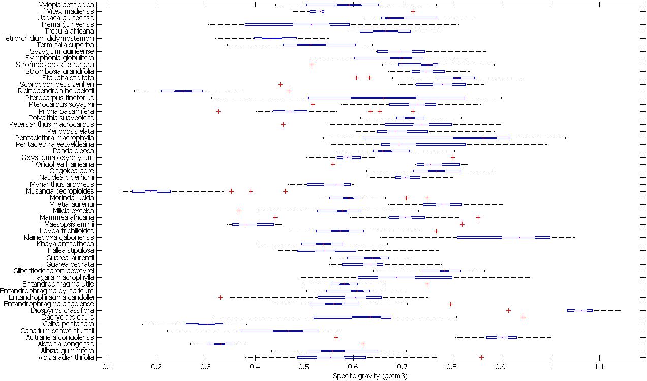
We observe a considerable variation in WSG within many species (Fig. 5). However, it is important to highlight that although some xylarium samples include information on tree location (with variable accuracy), the position in the tree from which the sample was drawn is not available. As it is well known that wood density can vary substantially within, as well as between trees ([37]), this might partially explain the large variations in some species. Furthermore, marked variations in WSG may be observed for a tree species which are attributable to differences in site quality and/or forest types ([23]) and site specific differences have been observed comparing the same species growing in different site conditions or forest types (e.g., [20], [21]).
Fig. 5 - Boxplot showing the inter-individual variation in WSG for the 53 measured species. The boxplot also shows the notches for each species: two medians are significantly different at the 5 percent significance level if their intervals (interval endpoints are the extremes of the notches) do not overlap. The figure also shows the whiskers of which the length w is set at 1.5. Points are drawn as outliers (crosses) if they are larger than q3 + w(q3 - q1) or smaller than q1 - w(q3 - q1), where q1 and q3 are the 25th and 75th percentiles, respectively. The whisker plotted on the figure extends to thewhich is the most extreme data value that is not an outlier.
Conclusion
The purpose of this paper was to: (1) highlight the potential use of xylarium samples to measure WSG; (2) provide an assessment on determining wood sample volume to calculate WSG from dry xylarium samples that have to be preserved in their original state; and (3) contribute and compare the WSG values of the 53 measured species in the Congo Basin Forest to existing databases and present a preliminary ecological assessment of the interindividual variation in WSG and the representativeness of genus-level averages compared to species-level averages.
To estimate wood volume of xylarium samples to calculate WSG, we generallyrecommend the hydrostatic approach of not wrapping samples in laboratory parafilm. As the impact on WSG of correcting for absorption is negligible, this is not necessary. Comparing the hydrostatic method for samples not wrapped in parafilm but correcting for absorption to the other two hydrostatic methods (i.e., either with parafilm, or without parafilm but without correction for absorption) and the glass microbeads method resulted in a high r 2 value (> 0.95). This suggests that any of these other three methods are valid depending on the limitations of the samples one would be working with and the objectives of the study. Hence, we have shown the validity of using laboratory parafilm to wrap samples for the hydrostatic method and the glass microbeads construction. When samples cannot be immersed in water in any circumstances, the glass microbeads construction offers a reliable alternative. When possible, using sterile water instead of tap water may further increase the precision of the hydrostatic methods.
This study also illustrates the contribution that the measurement of xylarium samples can make to existing global wood density databases. This contribution consists both in adding species that are currently not present in the database, but also helping to improve the current database estimates by increasing the number of measurements. Although the data presented is by no means extensive, it does illustrate the intervariability in WSG within and between species and suggest that genus-level WSG averages may indeed be representative of species-level WSG averages in the Congo Basin.
In a broader context, we have illustrated that, although working with xylarium samples brings several methodological challenges, these can be overcome to enable the use of xylarium samples to calculate WSG. In this way, xylaria hold a great amount of untapped information on taxonomic, spatial and potentially temporal variation in wood specific gravity that could be useful for ecologists, especially for providing more robust estimates of aboveground biomass and understanding of forest dynamics.
Acknowledgments
We thank Pol Dricot for constructing the glass microbeads machines and the handling of samples for testing the accuracy of the glass microbeads method. We also thank Nicolas Barbier and three reviewers for helping us to improve the manuscript.
References
CrossRef | Gscholar
Gscholar
CrossRef | Gscholar
Gscholar
Gscholar
CrossRef | Gscholar
Gscholar
Gscholar
Gscholar
Gscholar
Gscholar
Gscholar
Authors’ Info
Authors’ Affiliation
Y Malhi
Environmental Change Institute, School of Geography and the Environment, Dyson Perrins Building, South Parks Road, OX1 3QY Oxford (UK)
CIRAD, UMR Eco & Sols, Ecologie Fonctionnelle, Biogéochimie des Sols & Agroécosystèmes, place Viala, F-34060 Montpellier (France)
INRA, UR BEF - Biogéochimie des Ecosystèmes Forestiers, F-54280, Champenoux (France)
Walloon Agricultural Research Centre (CRA-W), chaussée de Namur 146, B-5030 Gembloux (Belgium)
Laboratory for Wood Biology and Xylarium, Royal Museum for Central Africa, Leuvense Steenweg 13, B-3080 Tervuren (Belgium)
Corresponding author
Paper Info
Citation
Maniatis D, Saint André L, Temmerman M, Malhi Y, Beeckman H (2011). The potential of using xylarium wood samples for wood density calculations: a comparison of approaches for volume measurement. iForest 4: 150-159. - doi: 10.3832/ifor0575-004
Academic Editor
Marco Borghetti
Paper history
Received: Sep 15, 2010
Accepted: May 16, 2011
First online: Aug 11, 2011
Publication Date: Aug 11, 2011
Publication Time: 2.90 months
Copyright Information
© SISEF - The Italian Society of Silviculture and Forest Ecology 2011
Open Access
This article is distributed under the terms of the Creative Commons Attribution-Non Commercial 4.0 International (https://creativecommons.org/licenses/by-nc/4.0/), which permits unrestricted use, distribution, and reproduction in any medium, provided you give appropriate credit to the original author(s) and the source, provide a link to the Creative Commons license, and indicate if changes were made.

Web Metrics
Breakdown by View Type
Article Usage
Total Article Views: 66240
(from publication date up to now)
Breakdown by View Type
HTML Page Views: 53283
Abstract Page Views: 5518
PDF Downloads: 5417
Citation/Reference Downloads: 34
XML Downloads: 1988
Web Metrics
Days since publication: 5454
Overall contacts: 66240
Avg. contacts per week: 85.02
Article Citations
Article citations are based on data periodically collected from the Clarivate Web of Science web site
(last update: Mar 2025)
Total number of cites (since 2011): 17
Average cites per year: 1.13
Publication Metrics
by Dimensions ©
Articles citing this article
List of the papers citing this article based on CrossRef Cited-by.
Related Contents
iForest Similar Articles
Research Articles
Estimation of total extractive content of wood from planted and native forests by near infrared spectroscopy
vol. 14, pp. 18-25 (online: 09 January 2021)
Research Articles
Physical, chemical and mechanical properties of Pinus sylvestris wood at five sites in Portugal
vol. 10, pp. 669-679 (online: 11 July 2017)
Research Articles
Characterization of VOC emission profile of different wood species during moisture cycles
vol. 10, pp. 576-584 (online: 08 May 2017)
Research Articles
NIR-based models for estimating selected physical and chemical wood properties from fast-growing plantations
vol. 15, pp. 372-380 (online: 05 October 2022)
Research Articles
Identification of wood from the Amazon by characteristics of Haralick and Neural Network: image segmentation and polishing of the surface
vol. 15, pp. 234-239 (online: 14 July 2022)
Research Articles
Dielectric properties of paraffin wax emulsion/copper azole compound system treated wood
vol. 12, pp. 199-206 (online: 10 April 2019)
Research Articles
Physical and mechanical characteristics of poor-quality wood after heat treatment
vol. 8, pp. 884-891 (online: 22 May 2015)
Research Articles
Characterization of technological properties of matá-matá wood (Eschweilera coriacea [DC.] S.A. Mori, E. odora Poepp. [Miers] and E. truncata A.C. Sm.) by Near Infrared Spectroscopy
vol. 14, pp. 400-407 (online: 01 September 2021)
Research Articles
Comparison of alternative harvesting systems for selective thinning in a Mediterranean pine afforestation (Pinus halepensis Mill.) for bioenergy use
vol. 14, pp. 465-472 (online: 16 October 2021)
Research Articles
Density, extractives and decay resistance variabilities within branch wood from four agroforestry hardwood species
vol. 14, pp. 212-220 (online: 02 May 2021)
iForest Database Search
Search By Author
Search By Keyword
Google Scholar Search
Citing Articles
Search By Author
Search By Keywords
PubMed Search
Search By Author
Search By Keyword


