Modelling the moisture status of habitats by using NDVI on the example of the Cerrado and Atlantic Forest biomes borderland (Brazil)
iForest - Biogeosciences and Forestry, Volume 18, Issue 6, Pages 375-381 (2025)
doi: https://doi.org/10.3832/ifor4413-018
Published: Dec 16, 2025 - Copyright © 2025 SISEF
Research Articles
Abstract
The Brazilian Cerrado and the Atlantic Forest are important global biodiversity hotspots that are highly diverse in geological structure, soil, and climatic conditions, all of which directly affect vegetation diversity. The conservation of these biomes depends on recognizing variations in their humidity levels. Given the correlation between water access and plant health, as illustrated by NDVI, we assessed the feasibility of building an NDVI-based model to detect variations in habitat moisture. Using various statistical algorithms, the correctness of the NDVI-based habitat moisture assessment model was confirmed. In addition, it was determined that UMAP was the most favourable of the algorithms employed. Our method provides a practical, efficient tool for assessing habitat moisture that can benefit fields such as ecology, conservation biology, and land management.
Keywords
Ipanema National Forest, NDVI, UMAP Algorithm, Habitat Moisture Index
Introduction
All ecosystems on Earth depend on water. Several methods are used for detecting differences in the moisture status of terrestrial ecosystems and monitoring changes in their hydrological conditions, such as remote sensing ([17]), ground-based measurements ([32]), hydrological models ([1]), and carbon and water flux measurements ([4]). All these methods can identify moisture differences in terrestrial biomes and monitor hydrological changes over time. However, there is a persistent demand for cost-effective, easy-to-apply techniques, particularly for valuable natural areas. Among the most important biomes on the globe are the Brazilian Cerrado, considered a biodiversity hotspot, and the Atlantic Forest. The Cerrado is situated in central Brazil, and is the second-largest of Brazil’s major biomes, following Amazonia. It comprises woodlands, savannas, grasslands, as well as gallery and dry forests ([16]). Kisselle et al. ([15]) distinguish two types of Cerrado: the cerrado sensu stricto (20-50% canopy cover) and the cerrado campo sujo (open, scrubland, <10% canopy cover). This biome hosts some 4.800 species of plants and vertebrates found nowhere else ([29]). Despite its enormous importance for species conservation, as little as 19.8% of the Cerrado remains undisturbed, the majority having been transformed into pasture and other forms of agricultural land use ([30]). The idea of monitoring the Brazilian Cerrado using spectral indices dates back many years. In 2004, Ferreira and Huete described the seasonal dynamics of this biome using NDVI and the Soil Adjusted Vegetation Index (SAVI), analysed in five seasonal periods: (1) summer rains (from January to March), (2) dry winter (from April to August), (3) end-of-the-drought period (September), (4) beginning of the rainy season (October), and (5) spring rains (November and December). These authors identified three major spatial domains of the Cerrado: (i) the “true” Cerrado formations and pasture sites, (ii) the forested areas (seasonal broadleaf and dense Cerrado woodland), and (iii) agricultural crops. They concluded that “the use of multiple indices should improve vegetation studies”.
The Atlantic Forest (AF) is the second-largest tropical forest in South America and one of the most biodiverse biomes worldwide. Brazil owns most of the AF (93% of the total area), with the remainder belonging to Paraguay (5.3%) and Argentina (1.7%) ([19]). The AF is classified as one of three major biodiversity hotspots, together with the Cape Floristic Region and Polynesia-Micronesia region, and is particularly vulnerable to climate change ([2]). The altitudes of the AF vary from sea level to 2891 m, with the relief ranging from depressions to mountains. The climate is extremely diverse, including tropical rainforest (Af); tropical monsoon (Am); tropical savannah (Aw); arid hot steppe (BSh); and temperate, without dry season; with hot (Cfa) and warm (Cfb) summers and temperate dry winters (Cw). Soils vary widely, from dystrophic to eutrophic ([19]).
A common feature of the AF is the existence of two annual cycles. According to Da Silva et al. ([6]), vegetation in Caparaó National Park (Brazil) and its buffer zone is highly dependent on precipitation, with a strong correlation between precipitation and vegetation indices. Tests of the relationships between forest and vegetation indices conducted in the Atlantic Rainforest on the Atlantic slope of Serra do Mar ([11]) concluded that MVI5 (moisture vegetation index using Landsat’s band 5) and MVI7 (moisture vegetation index using Landsat’s band 7) showed the best performances in dense humid forests. In contrast, NDVI was a good indicator for deciduous and dry forests. However, the usefulness of NDVI for ecological research has been demonstrated by multiple authors worldwide ([24], [34]). Studies on the vegetation at the border of the Cerrado and the Atlantic Forest should help protect these biomes and clarify the relationships between vegetation and habitat conditions.
In this study, we examined the use of NDVI to assess moisture conditions in ecosystems, using the Ipanema National Forest (INF) as a case study. This forest is located at the boundary between the Brazilian Cerrado and the Atlantic Forest biomes. It was assumed that (i) the water accessible to plants is affected by the sum and distribution of atmospheric precipitation and the differentiated water retention capacity depending on the variability of the terrain properties (land relief, geology, soils), (ii) the humidity level of the habitat affects the diversity of the vegetation cover, and (iii) the NDVI values of the vegetation depends on the amount of available water. Based on these assumptions, the hypothesis was formulated that habitat moisture levels, influenced by vegetation, could lead to differences in NDVI. These variations in NDVI values could then be used to assess differences in habitat moisture. The aim of the study was to develop a mathematical model based on NDVI, vegetation types, and various habitat conditions to monitor changes in habitat moisture. NDVI has not yet been used in this context. This information can help understand how ecosystems are responding to climate change and other environmental stressors.
Material and methods
Study area
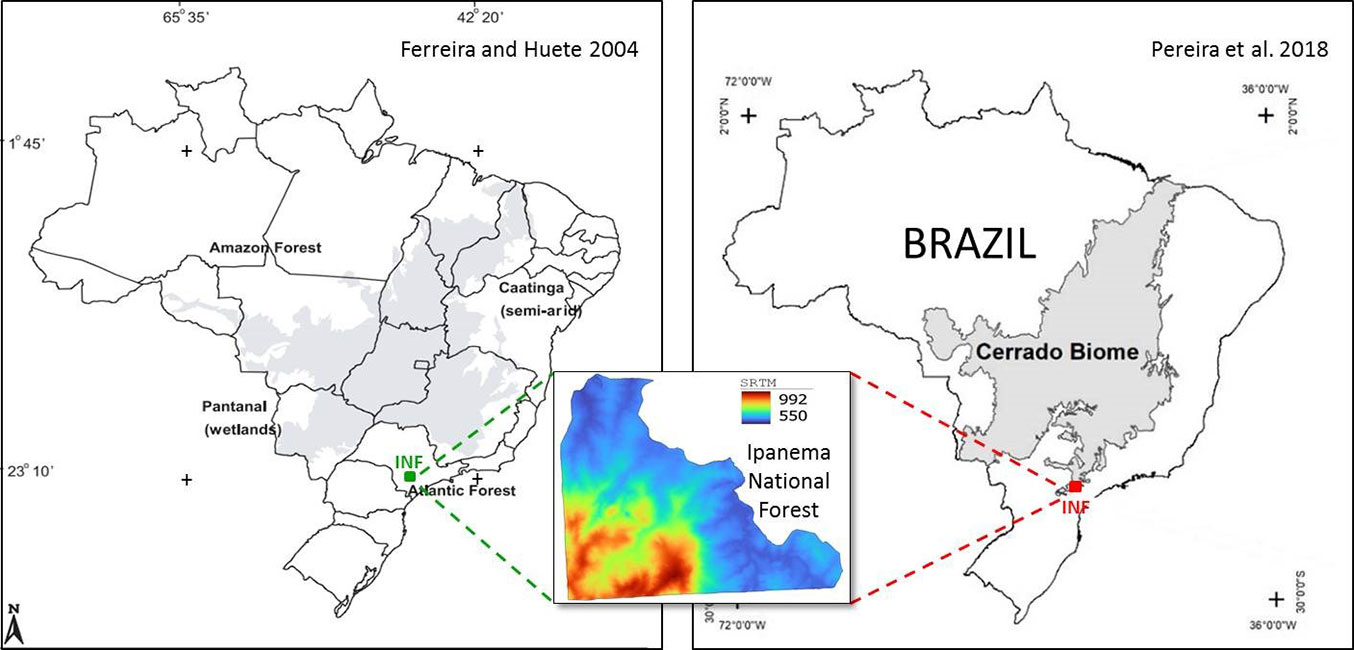
The Ipanema National Forest (INF) is a poorly studied protected area ([18]). It encompasses approximately 5.000 ha, of which 75% is covered by semideciduous (90% of all forests) and rainforests in several successional stages ([3]). Due to extensive exploitation of tree species over the last two centuries, the vegetation consists of secondary forests ([27]). The topography of the INF is highly diversified, and the soil is clay and rocky ([26]). From September to February, the climate is wet, while it is dry from March to August ([3]). According to Ferreira & Huete ([9]), the territory lies within the Atlantic Forest biome; according to Pereira et al. ([22]), at the southern range of the Cerrado biome (Fig. 1).
Satellite data
Image data from the Sentinel-2 (A, B) satellites of the European Space Agency (ESA) were used for the analysis. The satellites are equipped with an MSI sensor with characteristics listed on the ESA website (⇒ https://sentinels.copernicus.eu/web/sentinel/user-guides/sentinel-2-msi). They are installed on two platforms, namely S2A and S2B. Image data were imported into Google Earth Engine™ (GEE) and subjected to the automatic cloud cover assessment. Data from the Level L2A product were used for the analysis. It means that each image pixel for the spectral band contains a calibrated reflectance of the Earth’s surface and was created as a result of geometric correction that accounts for atmospheric radiation changes. In GEE, images with a cloud ratio of less than 10% with a defined INF area were selected. For this purpose, the SCL (Scene Classification Layer) was used. On this layer, areas with the following values were identified: shadows -3, clouds with low probability -7, medium -8, high -9, cirrus clouds -10. Areas with medium and high probability were excluded when their number of pixels was greater than 50. In total, 61 images from 2018 to 2021 were selected. For all images, NDVI was utilized for calculations. As shown in Tab. 1, the differences between Sentinel 2A and 2B are not significant and were therefore considered insignificant for the purposes of these studies.
Tab. 1 - Sentinel 2 channels used in the NDVI calculations (⇒ https://sentinel.esa.int/web/sentinel/technical-guides/sentinel-2-msi/msi-instrument).
| Sentinel 2 Bands | B4 | B8 |
| Spatial resolution (m) | 10 | 10 |
| Sentinel 2A central wavelength (nm) | 664.5 | 835.1 |
| Sentinel 2B central wavelength (nm) | 665.0 | 833.0 |
| Sentinel 2A bandwidth (nm) | 38.0 | 145.0 |
| Sentinel 2B bandwidth (nm) | 39.0 | 133.0 |
| Other Characteristics | pigment chlorophyll absorptions in the red band ([31]) | responsive to canopy structural variations, canopy type, and architecture ([31]) |
NDVI was calculated in GEE. The multilayer file was downloaded and analyzed using QGIS ver. 3.22.8. The quality of RGB images was visually assessed, and images with visible defects were discarded. In addition, a plug-in from the website ⇒ http://terrabrasilis.dpi.inpe.br/ was installed to enable the addition of another layer of the Cerrado forest ranges and Atlantic Forest biomes. Habitat layers were taken from Willmersdorf ([33]). The habitat and biome range layers were multiplied by and subtracted from each other, and the resulting boundary layer was used for calculations and for visualizing NDVI values. The calculations were performed using the zonal statistics plug-in, using the boundary layer and the NDVI map. The plug-in is a standard QGIS plug-in that converts a raster layer to a vector layer and calculates variable statistics for a given area, such as sum, mean, deviation, and median.
Determination of the habitat moisture index
To determine the habitat moisture index, the following data were used: (i) data on precipitation for the years 2018-2021 taken from the Fezenda Ipanema Airport meteorological station (METAR), located 300 m from the eastern border of the research area; this data provided the total precipitation per hour, with 24 measurements per day. (ii) A relief map generated based on the global elevation model SRTM 30 m ([8]). (iii) A map of geological formations obtained from Willmersdorf ([33]). (iv) A soil map obtained from Willmersdorf ([33]). (v) A map of vegetation types generated based on Willmersdorf ([33]).
The classification of habitats into wet, humid, mesic, and dry categories is based on the total atmospheric precipitation, which was compiled as average values for 14-day periods. This classification was related to changes in NDVI values, as illustrated in Fig. S2 (Supplementary material). According to the yearly trend, it was assumed that the data for the first quarter of the year (January-March) correspond to the wet period, and those for the third quarter (July-September) correspond to the dry period. The second and fourth quarters (April-June and October-December, respectively) were considered transitional periods and classified as “humid” and “mesic”, respectively.
Similarly, a subdivision of the year into 4 quarters was adopted for analyzing NDVI data: (i) January to March; (ii) April to June; (iii) July to September; (iv) October to December. Each quarter was assigned colors corresponding to four classes of decreasing humidity: (i) wet - blue and light blue; (ii) humid - green; (iii) mesic - yellow; (iv) dry - red. To calculate the humidity index of habitats, it was assumed that: (i) class “g1” (wet) are areas where the contour of the blue and light blue colours are present in all four quarters of the year; (ii) class “g2” (humid) are areas where the contour of the blue and light blue colours are present in three quarters; (iii) class “g3” (mesic) are areas where the contour of the blue and light blue colours are present in only two quarters; (iv) class “g4” (dry) are areas where the blue and light blue colours are present in only one quarter of the year. By employing applied mathematical algorithms, a model was developed to determine the contours of the areas for g1-g4 classes based on the images. Finally, the habitat moisture index was determined by linking the contours of the habitat moisture levels determined by the model with vegetation, precipitation, soils, terrain, and geological formations.
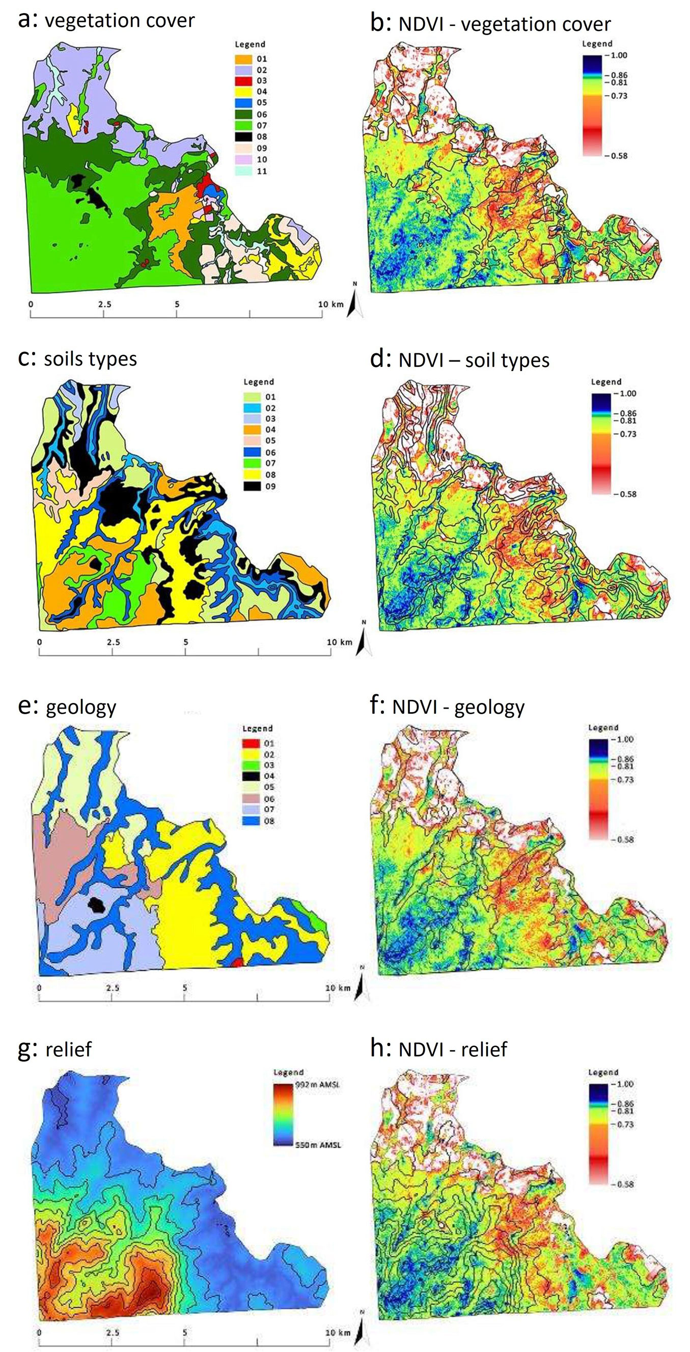
The model validation involved analyzing results in relation to soil and terrain features that are closely associated with moisture, e.g., the relief of a river valley (Fig. 2g), which collects precipitation water, and fluvisols (Fig. 2c), which are soils particularly dependent on the river water level.
Fig. 2 - Comparison of differentiation of INF vegetation cover (2a), soil types (2c), geology (2e) and relief (2g) on the background of average (2018-2021) NDVI values in relation to the contours of vegetation (2b), soils (2d), geology (2f) and relief (2h). Legend to Figure 2a: 1 - Rocky Outcrop (Grasses/Shrubs) [Portuguese: Afloramento Rochoso (Gramineas/Arbustivas)]; 2 - Agriculture (Pasture/Cultivation) [Agropecuaria (Pastagens/Cultivos)]; 3 - Urban Area (Buildings/Towns) [Área Urbana (Edificações/Vilas)]; 4 - Cerrado (Campo Sujo); 5 -Water Bodies (Reservoirs) [Corpo d’Água (Reservatórios)]; 6 - Forest in Regeneration (Floresta em Regeneração); 7 - Seasonal Semideciduous Forest (Floresta Estacional Semidecidual); 8 - Mining (Cavages/Buildings) [Mineração (Cavas/Edificações)]; 9 - Reforestation (Exotic) [Reflorestamento (Exóticas)]; 10 - Reforestation (Native) [Resflorestamento (Nativas)]; 11 - Floodplain [Várzea (Alagados/Brejos)]. Legend to Figure 2c: 1 - Acrisols (In Portuguese Argissolo Vermelho Amarelo Distrófico); 2 - Gleysols (Gleissolo); 3 - Ferralsols (Latossolo Amarelo); 4 - Ferralsols (Latossolo Vermelho Distrófico); 5 - Neossolo Litólico Afloramento (no equivalent in [14]); 6 - Fluvisols (Neossolo Flúvico); 7 - Neossolo Latólico Listico (no equivalent in [14]); 8 - Neossolo Litólico Distrófico ([14]); 9 - Neossolo Litólico Húmido ([14]). Legend to Figure 2e: 1 - Amphibolite (Portuguese: Anfibolito); 2 - Conglomeratic Sandstone (Arenito Conclomeratico); 3 - Claystones (Argilito); 4 - Basic eruptive: basalt (Eruptivas basicas basalto); 5 - Stratified rock, verve (Folhelho Varvito); 6 - Porphyroid-granite (Granito porfiroide); 7 - Alkaline Intrusives: Shonkinite-porphyry (Intrusivos Alcalinas Shonkinito-porfito); 8 - Quaternary (Quaternario).
Statistical analysis
The primary goal of the statistical analysis was to assess whether the 38 parameters, categorized into four groups (altitude, vegetation, soils, and geology), could validate the classification of INF habitats into four moisture groups (g1-g4). These groups were based on habitat moisture as derived from NDVI and other related parameters. The aim was to confirm the accuracy of the NDVI-based habitat humidity assessment model, rather than prove that NDVI indicates humidity.
Three tools were used for the above purpose: the study of the covariance matrix, two dimensionality reduction algorithms (PCA and UMAP), and a g1-g4 classifier built using the adopted parameters. The UMAP algorithm (⇒ https://arxiv.org/abs/1802.03426) is far more promising than PCA. UMAP focuses on a low-dimensional representation that best reflects the topological structure of the original (high-dimensional) data. It is an alternative to the t-SNE method, a commonly used nonlinear dimension reduction algorithm. UMAP produces similar or better representations, as it retains more global data features, and its output is more stable. Moreover, UMAP is more efficient than t-SNE in both dimensionality and data size.
To construct a classification model of classes g1-g4 based on 38 parameters, we tested five classification algorithms: (i) linear discriminant analysis (LDA); (ii) quantitative descriptive analysis (QDA); (iii) logistic regression; (iv) support vector machine (SVM); (v) Random forest.
All calculations were made using Python and the scikit-learn library (⇒ https://scikit-learn.org/stable/). The dataset used consisted of 510 cases, classified into classes g1-g4 according to 38 parameters: 11 classes of vegetation cover, 10 classes of altitude, nine classes of soil, and eight classes of geological formations. The INF area was divided into 1×1 km squares, creating distinct sets in which classes g1 through g4 were established. Each square contained a variety of habitat conditions and vegetation types, allowing us to treat each square as a separate sample (Fig. S1 in Supplementary material). For each tested model, learning curves were generated ([12]), and the accuracy and mean square error of the model were recorded.
The methods were tested on training and validation datasets as a function of the amount of training data. The “LearningCurveDisplay.from_estimator” function, which visualises the method’s error as negative values, was used to generate the curves, where higher values indicate higher quality (⇒ https://scikit-learn.org/stable/modules/model_evaluation.html#scoring-parameter). The cross-validation level was set to 30. Graphs were created for seven tested algorithms. As for the SVM algorithm, three kernels were tested: linear functions, polynomial functions (e.g., a fifth-degree polynomial), and radial basis functions.
Results
The analysis of NDVI-based images showed that INF vegetation is clearly rainfall-dependent, as reflected by its partition into dry and wet seasons (Fig. S2 in Supplementary material). It also highlighted the relationships between vegetation, soil types, geological formations, and relief.
Fig. 2shows the diversity of vegetation cover (2a, 2b), soil types (2c, 2d), geological formations (2e, 2f), and relief (2g, 2h) compared to NDVI diversity.
Statistical analysis
Covariance matrix analysis (Fig. 3) revealed that: (i) altitude parameters are weakly or very weakly correlated with parameters belonging to other groups; the maximum correlation values and the percentage of zeros for individual groups were, respectively, 0.09 and 0.7 with the parameters of the vegetation group, 0.18 and 0.73 with the group of geological parameters, and 0.19 and 0.74 with the group of soil parameters; (ii) the group of vegetation parameters was fairly correlated with the group of geological parameters and the group of soil parameters; the maximum correlation values and the percentage of zeros for individual groups were respectively: 0.49 and 0.33 with the group of geological parameters, 0.41 and 0.13 with the group of soil parameters; (iii) the group of geological parameters was fairly correlated with the group of soil parameters; the maximum correlation value was 0.72, while the percentage of zeros was 0.1. This suggests considering class parameterisation limited to the altitude block and one of the other three blocks.
Fig. 3 - Covariance matrix. Green boxes indicate high parameter dependence; orange boxes indicate fields excluded from the correlation analysis; the individual blocks of the tested parameters were separated using sand, blue, and grey colours.
The PCA algorithm results indicated that trying to reduce the parameter space dimension with a linear model is likely to fail. Fig. S3 (Supplementary material) shows the percentage distribution of the degree of explanation for all principal components. The quantitative impact of the original parameter values for the first ten principal components is visualised in Fig. S4. It is clearly visible that the three blocks (vegetation, geology, and soil) equally strongly affect their construction, which suggests their mutual redundancy.
Fig. S5 illustrates the 510 examined cases projected onto the first two UMAP components. The poor separation of groups g1 and g4 does not concern the natural habitat conditions in the field, but the presentation of the UMAP analysis results in a multidimensional space (38 dimensions). The overlap between groups g1 and g4 may reflect their narrow range of habitat conditions (although completely different), and thus fewer occurrences, which makes the groups more mathematically similar to each other. However, it is worth noting that on the horizontal axis, within the range 4 to 5.5, there is an apparent clustering of points representing group g1.
The separation of groups g1 to g4 is not perfect, but it is adequate to validate the selection criteria used for distinguishing these moisture groups. Given the different ontologies of the 38 parameters, the universal Euclidean metric was employed to measure the distance between them. Additionally, a value of seven was assumed for the number of neighbors when estimating the similarity measure. This choice suggests a reasonable level of “local” calculations within the 38-dimensional space.
The accuracy and the error rate of the learning curves are presented in Fig. S6 (Supplementary material), where the averaged (smoothed) curves for the training and validation sets are reported, along with their variance (indicated by the lighter bands surrounding the curves). Based on the analysis of these graphs, we can draw the following key considerations. (i) The 510 samples used are adequate to achieve stable results, as indicated by the flattening curves. (ii) Two methods, LDA and SVM-poly, demonstrated abnormally low accuracy. The significant increase in SVM-poly’s accuracy around 470 training cases, after prior stabilization, is likely a numerical anomaly. (iii) In all cases, except for SVM-poly, the variance of the training set decreases (improving or worsening) as its size increases. This suggests that the information quality of the training set is relatively good. (iv) A high variance in the validation set coupled with a low variance in the training set indicates that the model is overfitting, meaning it was too rigidly tailored to the training data. This is evident in all cases except SVM-RBF and QDA. In QDA, a training set larger than 200 cases increased the variance, with additional data adding only noise, and results stabilizing before reaching 200. Possible strategies to reduce overtraining include testing a wider range of standard regularisation parameters and modifying the parameter set by removing some and/or adding new ones, which is more difficult both conceptually and in terms of cost. The analysis of covariance described above supports the reduction of highly correlated groups.
A relatively small variance was observed in the validation set across specific ranges of training set size for the random forest algorithm. A general upward trend in this variance (similar to QDA) suggests that information noise increases as the size of the training set grows.
The above results prompted us to test three algorithms using a reduced set of parameters, consisting of the two blocks height and vegetation. In the case of the QDA algorithm, this set proved numerically unstable. The learning curves for the other two cases (SVM-RBF and random forest) are shown in Fig. S7 and Fig. S8 (Supplementary material). In both cases, minimal loss in accuracy was observed, along with a reduction in the validation set’s variance, especially with random forests. This demonstrates that the SVM-RBF and random forests algorithms achieve fairly good classification of the defined moisture classes with the adopted set of parameters, thereby confirming the adequacy of the class g1-g4 definitions.
The significance of the altitudinal parameters group was further confirmed when a classifier was developed using only parameters from the vegetation, geological, and soil groups. This is illustrated by the learning curve for the random forest algorithm (Fig. S8), which reveals a marked decrease in accuracy and a considerable increase in variance for both the training and validation sets.
Summary of results
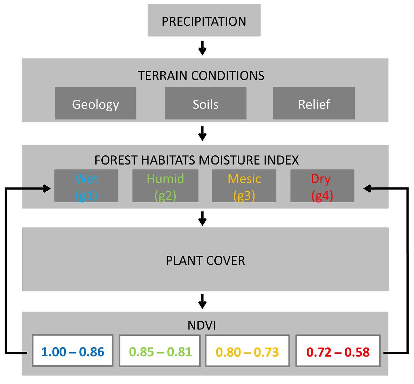
NDVI value ranges were assigned to the different humidity levels in the study area based on the aforementioned analyses. When the average annual NDVI value was in the range 1.00-0.86, the habitat was considered wet (g1); when it was 0.85-0.81, the habitat was considered moist (g2); habitats with average annual NDVI within the range 0.80-0.73 were considered mesic (g3); while when average annual NDVI was below 0.73, the habitat was considered dry (g4).
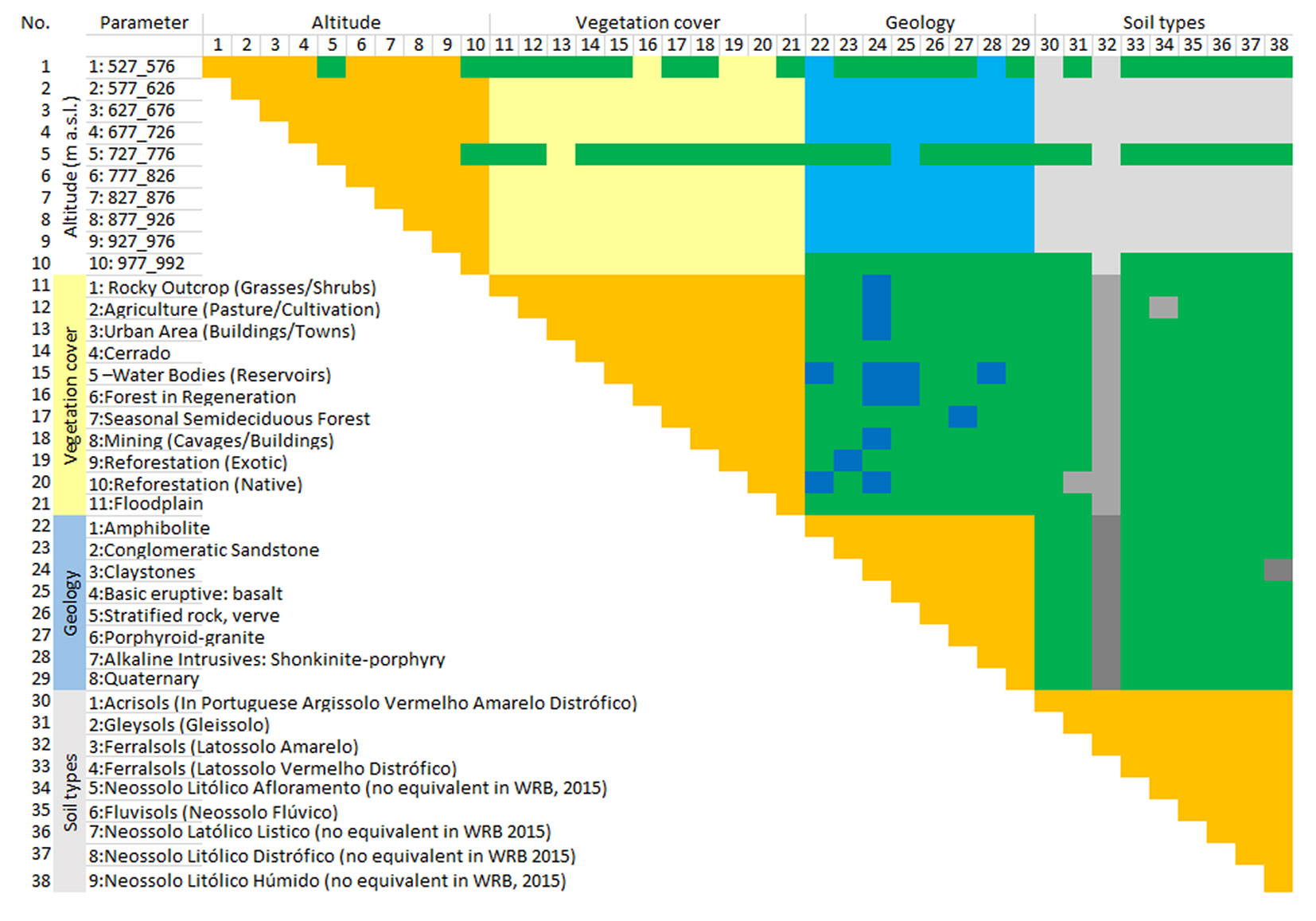
The diagram of the relationships among individual parameters, NDVI values, and habitat moisture classes for the INF is shown in Fig. 4.
Fig. 4 - Relationships among individual parameters, NDVI values, and habitat moisture classes for INF.
Discussion
Studies on NDVI have revealed complex relationships among this index, meteorological factors, soil moisture, and vegetation cover type ([5], [23], [13], [34]). Our results from the Ipanema National Forest confirmed that a complex set of factors, including climate, relief, altitude, geology, and soil type, affects vegetation cover and its moisture status. According to Mazón et al. ([20]), the effects of elevation on various forest characteristics remain poorly understood. Regardless of habitat conditions, forests are primarily found in the higher mountainous regions of the study area, likely due to the inaccessibility of these areas, which makes them unsuitable for agricultural development. At the same time, seasonal semideciduous forests (Fig. 2) had the highest average NDVI values from 2018 to 2021. This is due to the river valley’s relief (Fig. 2g), where fluvisols (Fig. 2c) developed by collecting water from precipitation, thus supporting the link between terrain and soil. Gleysols, associated with high humidity ([28]), are also found in this area. However, the average NDVI values for 2018-2021 in these soils are markedly lower (Fig. 2c). This may be due to different vegetation cover, which is mainly composed of plantations of alien species on gleysols. The most planted forest species in South America is eucalyptus ([10]), which may change the natural water regime ([25]). Eucalypt monocultures are also present in the INF ([18]).
Among the different types of plant cover, cerrado campo sujo is noted in the INF (Fig. 2a), which would confirm the range of this biome given by [22] (Fig. 1). At the same time, these are lower, more easily accessible mountain locations; therefore, their transformation may be affected by human activities. The share of agricultural and urbanised areas in the lower part of the study area seems to confirm it (Fig. 2a). At the same time, it is a low-moisture area (Fig. 2b) that corresponds to the characteristics of the Cerrado described by Ferreira & Huete ([9]). These authors noted that the Cerrado region extends much farther north of the INF. Given the 14-year gap between the studies conducted by Ferreira & Huete ([9]) and Pereira et al. ([22]), this suggests that the increasing human pressure in the INF surrounding has forced forests into more remote areas.
The Cerrado biome, characterized by its canopy cover, animal grazing, land conversion into pasture and agriculture, and moisture conditions, is similar to the type of vegetation noted in the central part of Poland (European xero-thermophile oak woods - [7]), a region where the lowest precipitation and NDVI values were shown (Fig. S9 in Supplementary material). This is also the most deforested lowland part of the country, where human activity has led to the disappearance of natural hornbeam and oak forests. At the same time, it is unclear whether xero-thermophile oak woods thrive in the central part of the country because of the drier climate or if deforestation has caused the climate to become drier. To some extent, a similar phenomenon may occur at the border between the Cerrado and the Atlantic Forest, which is strongly influenced by human activity.
Our results confirm the relationship between NDVI and the moisture content of forest areas. Fig. S9 (Supplementary material) shows that the adopted method for assessing habitat moisture status is universal and can be applied worldwide.
Comparing the Brazilian Cerrado to the European xerothermophile oak woods involves examining how human activities impact forest management. This includes practices such as livestock grazing and the conversion of forested areas into agricultural land and pastures. Although a more comprehensive analysis of this comparison could be the focus of a separate study, this example illustrates that geographically distant forest ecosystems can be compared quickly and affordably. However, to effectively interpret the data, it is necessary to use a combination of satellite techniques and terrestrial data. Key factors to consider include vegetation cover diversity, soil diversity, and terrain variations. This approach was exemplified by the case study of the Ipanema National Forest.
Conclusions
The Normalized Difference Vegetation Index (NDVI) is widely used for estimating vegetation greenness and moisture content. However, our results proved that NDVI can also be used to build reliable models for assessing habitat moisture. Among the algorithms tested, UMAP was found to be the most effective. By using average NDVI values from 2018 to 2021, we classified the study area into four moisture classes: g1 (wet habitat - average NDVI = 1.00-0.86), g2 (moist - 0.85-0.81), g3 (mesic - 0.80-0.73), and g4 (dry - average NDVI value < 0.73).
The method used in this study is easy to apply, cost-effective, and provides high-resolution (10×10 m) data applicable to large geographical areas. The results showed that the method can be applied across diverse environmental conditions, including different vegetation cover types, soil types, and geological sediments. It can be used to assess habitat moisture diversity, compare moisture levels across habitats, and monitor them over time. For example, our study identified the boundary between two critical biomes, the Atlantic Forest and Cerrado, in the study area and suggested increased anthrogenic pressure in the surroundings of the INF, forcing forests into less accessible areas.
Overall, this method provides a practical, efficient tool for assessing habitat moisture that can benefit research fields such as ecology, conservation biology, and land management.
Acknowledgments
AM, MK, WK: conceptualization and methodology; AM, MK, KCT, WK: investigation; AM, SK, RHT: formal analysis; AM, MRM: visualization; AM, MK, WK, PR, SK, JP, KCT, RHT, MRM: original draft writing, review, and editing; AM: funding acquisition; AM, WK: funding acquisition and validation.
Funding Information
The study was financed by the project GEO-INTER-APLIKACJE no. POWR.03.02.00-00-I027/17, and co-financed by the European Union from the European Social Fund under the Operational Program Knowledge Education Development.
Conflicts of Interest
The authors declare no conflict of interest.
References
Gscholar
Gscholar
CrossRef | Gscholar
Gscholar
Gscholar
CrossRef | Gscholar
CrossRef | Gscholar
Authors’ Info
Authors’ Affiliation
Slawomir Królewicz 0000-0003-1117-7832
Jan Piekarczyk 0000-0002-2405-6741
Environmental Remote Sensing and Soil Science Research Unit, Faculty of Geographic and Geological Sciences, Adam Mickiewicz University in Poznan, Wieniawskiego 1, 61-712 Poznan (Poland)
Kelly Cristina Tonello 0000-0002-7920-6006
Rogerio Hartung Toppa 0000-0002-1637-2840
Marcos Roberto Martines 0000-0002-7464-2431
Department of Environmental Science, Federal University of São Carlos, Sorocaba (Brazil)
Pawel Rutkowski 0000-0003-3614-8923
Department of Botany and Forest Habitats, Faculty of Forestry and Wood Technology, Poznan University of Life Sciences, Wojska Polskiego 71F, 60-625 Poznan (Poland)
Department of Artificial Intelligence, Faculty of Mathematics and Computer Science, Adam Mickiewicz University in Poznan, Wieniawskiego 1, 61-712 Poznan (Poland)
Corresponding author
Paper Info
Citation
Mlynarczyk A, Konatowska M, Kowalewski W, Królewicz S, Tonello KC, Toppa RH, Martines MR, Piekarczyk J, Rutkowski P (2025). Modelling the moisture status of habitats by using NDVI on the example of the Cerrado and Atlantic Forest biomes borderland (Brazil). iForest 18: 375-381. - doi: 10.3832/ifor4413-018
Academic Editor
Davide Travaglini
Paper history
Received: Jul 04, 2023
Accepted: Jun 06, 2025
First online: Dec 16, 2025
Publication Date: Dec 31, 2025
Publication Time: 6.43 months
Copyright Information
© SISEF - The Italian Society of Silviculture and Forest Ecology 2025
Open Access
This article is distributed under the terms of the Creative Commons Attribution-Non Commercial 4.0 International (https://creativecommons.org/licenses/by-nc/4.0/), which permits unrestricted use, distribution, and reproduction in any medium, provided you give appropriate credit to the original author(s) and the source, provide a link to the Creative Commons license, and indicate if changes were made.

Web Metrics
Breakdown by View Type
Article Usage
Total Article Views: 2906
(from publication date up to now)
Breakdown by View Type
HTML Page Views: 1250
Abstract Page Views: 933
PDF Downloads: 621
Citation/Reference Downloads: 6
XML Downloads: 96
Web Metrics
Days since publication: 196
Overall contacts: 2906
Avg. contacts per week: 103.79
Article Citations
Article citations are based on data periodically collected from the Clarivate Web of Science web site
(last update: Mar 2025)
(No citations were found up to date. Please come back later)
Publication Metrics
by Dimensions ©
Articles citing this article
List of the papers citing this article based on CrossRef Cited-by.
Related Contents
iForest Similar Articles
Research Articles
Remote sensing of Japanese beech forest decline using an improved Temperature Vegetation Dryness Index (iTVDI)
vol. 4, pp. 195-199 (online: 03 November 2011)
Review Papers
Remote sensing-supported vegetation parameters for regional climate models: a brief review
vol. 3, pp. 98-101 (online: 15 July 2010)
Technical Reports
Detecting tree water deficit by very low altitude remote sensing
vol. 10, pp. 215-219 (online: 11 February 2017)
Review Papers
Accuracy of determining specific parameters of the urban forest using remote sensing
vol. 12, pp. 498-510 (online: 02 December 2019)
Research Articles
Landsat TM imagery and NDVI differencing to detect vegetation change: assessing natural forest expansion in Basilicata, southern Italy
vol. 7, pp. 75-84 (online: 18 December 2013)
Review Papers
Remote sensing of selective logging in tropical forests: current state and future directions
vol. 13, pp. 286-300 (online: 10 July 2020)
Technical Reports
Remote sensing of american maple in alluvial forests: a case study in an island complex of the Loire valley (France)
vol. 13, pp. 409-416 (online: 16 September 2020)
Research Articles
Assessing water quality by remote sensing in small lakes: the case study of Monticchio lakes in southern Italy
vol. 2, pp. 154-161 (online: 30 July 2009)
Research Articles
Mapping Leaf Area Index in subtropical upland ecosystems using RapidEye imagery and the randomForest algorithm
vol. 7, pp. 1-11 (online: 07 October 2013)
Research Articles
Assessing the influence of different Synthetic Aperture Radar parameters and Digital Elevation Model layers combined with optical data on the identification of argan forest in Essaouira region, Morocco
vol. 17, pp. 100-108 (online: 24 April 2024)
iForest Database Search
Search By Author
- A Mlynarczyk
- M Konatowska
- W Kowalewski
- S Królewicz
- KC Tonello
- RH Toppa
- MR Martines
- J Piekarczyk
- P Rutkowski
Search By Keyword
Google Scholar Search
Citing Articles
Search By Author
- A Mlynarczyk
- M Konatowska
- W Kowalewski
- S Królewicz
- KC Tonello
- RH Toppa
- MR Martines
- J Piekarczyk
- P Rutkowski
Search By Keywords
PubMed Search
Search By Author
- A Mlynarczyk
- M Konatowska
- W Kowalewski
- S Królewicz
- KC Tonello
- RH Toppa
- MR Martines
- J Piekarczyk
- P Rutkowski
Search By Keyword


