Mapping Leaf Area Index in subtropical upland ecosystems using RapidEye imagery and the randomForest algorithm
iForest - Biogeosciences and Forestry, Volume 7, Issue 1, Pages 1-11 (2014)
doi: https://doi.org/10.3832/ifor0968-006
Published: Oct 07, 2013 - Copyright © 2014 SISEF
Research Articles
Abstract
Canopy leaf area, frequently quantified by the Leaf Area Index (LAI), serves as the dominant control over primary production, energy exchange, transpiration, and other physiological attributes related to ecosystem processes. Maps depicting the spatial distribution of LAI across the landscape are of particularly high value for a better understanding of ecosystem dynamics and processes, especially over large and remote areas. Moreover, LAI maps have the potential to be used by process models describing energy and mass exchanges in the biosphere/atmosphere system. In this article we assess the applicability of the RapidEye satellite system, whose sensor is optimized towards vegetation analyses, for mapping LAI along a disturbance gradient, ranging from heavily disturbed shrub land to mature mountain rainforest. By incorporating image texture features into the analysis, we aim at assessing the potential quality improvement of LAI maps and the reduction of uncertainties associated with LAI maps compared to maps based on Vegetation Indexes (VI) solely. We identified 22 out of the 59 image features as being relevant for predicting LAI. Among these, especially VIs were ranked high. In particular, the two VIs using RapidEye’s RED-EDGE band stand out as the top two predictor variables. Nevertheless, map accuracy as quantified by the mean absolute error obtained from a 10-fold cross validation (MAE_CV) increased significantly if VIs and texture features are combined (MAE_CV = 0.56), compared to maps based on VIs only (MAE_CV = 0.62). We placed special emphasis on the uncertainties associated with the resulting map addressing that map users often treat uncertainty statements only in a pro-forma manner. Therefore, the LAI map was complemented with a map depicting the spatial distribution of the goodness-of-fit of the model, quantified by the mean absolute error (MAE), used for predictive mapping. From this an area weighted MAE (= 0.35) was calculated and compared to the unweighted MAE of 0.29. Mapping was done using randomForest, a widely used statistical modeling technique for predictive biological mapping.
Keywords
Ecosystem Monitoring, Forest and Vegetation Parameters, Leaf Area Index (LAI), Hemispherical Photography, Map Uncertainty, Vegetation Indexes, Image Texture, Xishuangbanna
Introduction
Canopy leaf area is the main factor for primary production, energy exchange, transpiration, and other physiological attributes related to ecosystem processes ([50], [31], [8], [65], [2]). The Leaf Area Index (LAI), defined as the projected leaf area per unit ground surface area, is frequently used to quantify the canopy leaf area. Thus, LAI is one of the key biophysical variables required by many process models describing the soil/plant/atmosphere system ([4], [39]). Because canopies and some of their characteristics can be directly observed from above, LAI is among the major variables of interest in remote sensing analyses ([40]), and its importance has led to considerable efforts to map its distribution over a variety of spatial and temporal scales ([16], [48], [74], [39], [63]). The majority of studies used (semi-) empirical relationships between LAI and combinations of spectral bands, namely vegetation indexes (VI), for LAI mapping ([4], [68]). In a review paper on the relationships between remotely-sensed VIs and canopy attributes, Glenn et al. ([29]) point out that VIs are often strongly related to light dependent physiological processes occurring in the upper canopy, but often exhibit only moderate relationships to detailed features of canopy architecture, such as LAI. VIs are generally regarded as important but have their limitations since they only utilize a fraction of the spectral information available in remote sensing data ([30]). Similarly, it has been pointed out that there is not enough evidence that spectral reflectance in the visible and near-infrared is sufficient to estimate LAI in forests, especially under close canopy situations ([40]). From their review, Glenn et al. ([29]) concluded that remote sensing models exclusively based on VIs to estimate LAI are, in particular, subject to error and uncertainty. Another fact to be considered is that LAI is a variable that cannot be directly measured in the field. Therefore, all efforts to correlate VIs derived from remote sensing interpretation to field observations are characterized by the lack of ground-level measurable parameters, as both information are results of modeling efforts.
Additional information derived from remote sensing images with the potential to improve LAI predictions are texture features. Texture features quantify the spatial variability of pixel values within a neighborhood defined by a moving window, and thus, complement the spectral information with a spatial component ([17]). As the variation in texture is related to changes in the spatial distribution of vegetation ([70]), image texture can be linked to the spatial distribution of vegetation ([17]).
The scope of this paper is to investigate the applicability of RapidEye imagery, which is optimized towards vegetation analyses, for LAI mapping along a disturbance gradient, ranging from heavily disturbed shrub-land to mature mountain rainforest. By incorporating image texture features into the analysis we aim at assessing the potential quality improvement of LAI maps and the reduction of uncertainties associated with LAI maps compared to those based on VIs solely ([29]). To predict LAI we use the Random Forest (RF) algorithm ([10]), an increasingly and widely used statistical modeling technique for predictive biological mapping ([51]).
Field data come from forest inventory plots located in the uplands of Xishuangbanna, China. Xishuangbanna is located in the transition zone between tropical southeastern Asia and subtropical and temperate China, resulting in the region with the highest biodiversity in China ([73], [42]). This high biological diversity is threatened by the expansion of rubber (Hevea brasiliensis) plantations ([71], [42], [72]). In the time from 1976 to 2003 Xishuangbanna’s estimated forest cover declined from 69% to less than 50% in conjunction with a decline of mean size of forest patches from 217 to 115 ha ([43]). The forest type most affected by the expansion of rubber plantations was tropical seasonal rain forest ([42]). For a better understanding of ecosystem dynamics and processes over large and remote areas, as faced in this region, LAI maps are of particularly high value ([14]).
Methods
Field data
The study site is located in Mengsong Administrative Village, Jinghong County, Xishuangbanna, Yunnan, China at an elevation of 800-2000 m a.s.l. (UTM/WGS84: 47N 656355 E, 2377646 N - Fig. 1). The sub-tropical climate of this region is influenced by the Indian monsoon; it has an annual mean temperature of 18 °C and an average rainfall of 1600-1800 mm, of which 80% is concentrated from May to October. Vegetation varies with altitude and the mosaic distribution of primary to secondary forest according to micro-environments.
Fig. 1 - Location of the study site Mengsong in Xishuangbanna, China. Black squares in Mengsong map depict the locations of the 28 inventory plots. Plots consist of 9 subplots arranged on a square grid with 50 meter spacing.
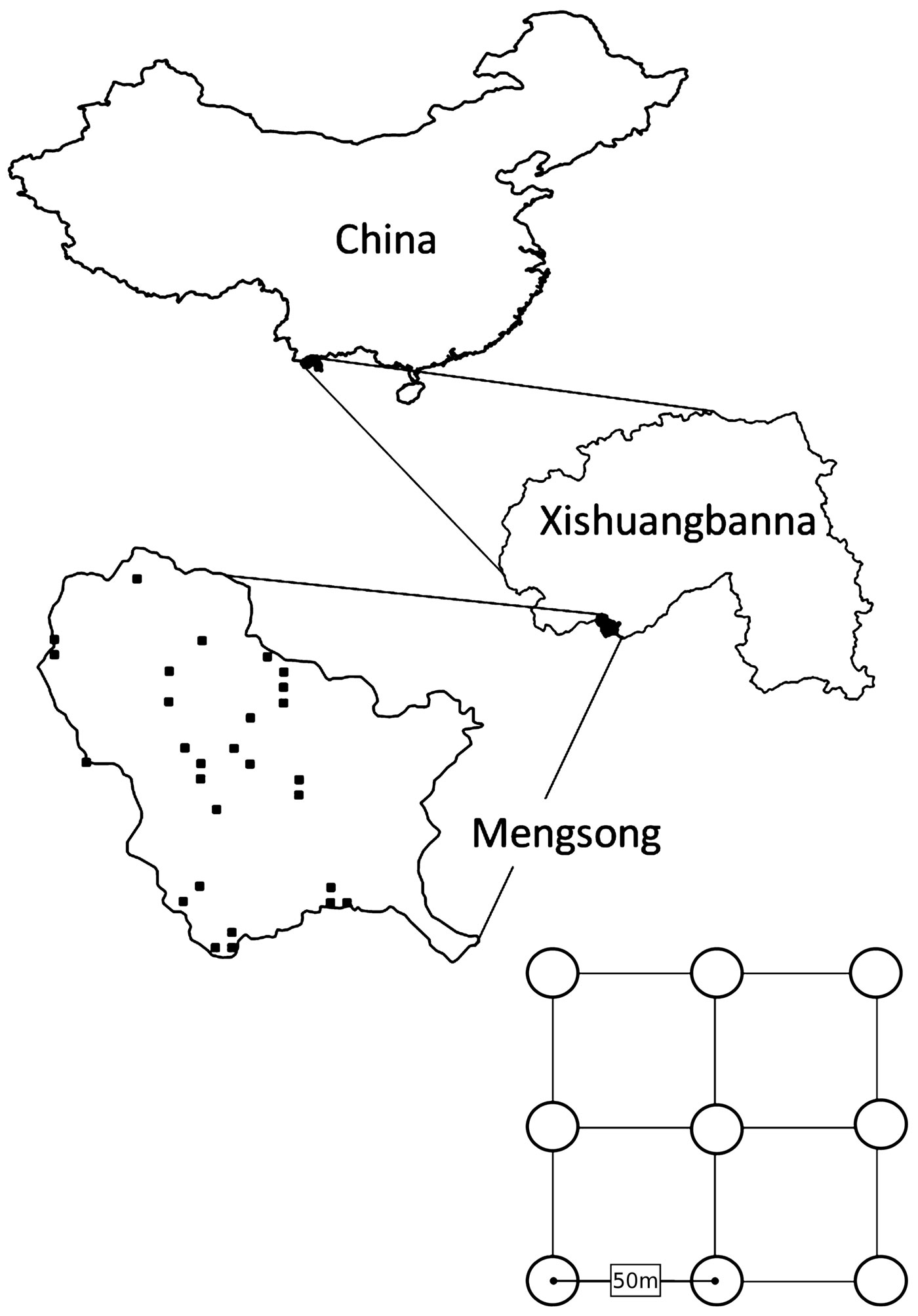
LAI data were assessed on 28 inventory plots in May 2011. Each plot consisted of nine subplots arranged on a square grid with 50 m spacing (Fig. 1, lower panel). Plots covered a gradient from heavily disturbed shrub land, through secondary regrowth to mature mountain rainforest. A probability sampling design was implemented: (1) to allow for a statistically sound assessment of LAI throughout the study site; and (2) because it contributes to scientifically defensible accuracy assessment ([58]). Plot locations were selected applying double sampling for stratification. A 500x500 m point grid was placed over the RapidEye image of the study site and each grid point classified into shrub land, regrowing forest, mature forest, and other land cover (e.g., settlements, water bodies, and mining claims). To ensure that sample plots were distributed over the whole area, the study site was divided into 16 equally sized primary units. From these primary units, 12 were randomly selected and within each one mature forest plot and one regrowing forest grid-point were selected at random. One shrub land grid-point was randomly drawn from every second of the selected primary units. The 28 selected grid-points became the SW corner of the sample plots.
At each subplot center, hemispherical photographs were taken with a Nikon D70s digital single lens reflex camera equipped with a Sigma Circular Fisheye 4.5 mm 1:2.8 lens with a field of view of 180°. The camera was mounted on a tripod at 1.2 m height to characterize the canopy without the interfering presence of understory vegetation ([62]). Vegetation within 0.5 m of the lens was removed, as this can lead to an inflation of the LAI estimate. The camera was leveled to face exactly the vertical using a bubble-level slotted into the flash socket. The camera was systematically orientated to magnetic north using a compass ([6]). Photographs were taken without direct sunlight entering the lens ([54]) in the early morning, late afternoon or on overcast days ([69]). The basic camera settings were mode “P” (Programmed Auto), ISO 400, and matrix metering. Photographs were underexposed by -2 stops of exposure ([37]) and stored in JPEG format (3008 x 2000 pixels resolution - [24]). To the blue color planes of the 8-bit photographs, an automated global thresholding was applied to avoid variations in threshold setting by manual interpretation of photographs and to speed up the processing time ([36], [20]). The “Minimum” thresholding algorithm ([52]) implemented in ImageJ ([56]) was used. From the binarized photographs, LAI was derived with Gap Light Analyzer 2.0 ([23]).
Remote sensing data
The RapidEye satellite system is optimized towards vegetation analyses and monitoring of agricultural and natural resources at relatively large cartographic scale ([64]). RapidEye’s 5 spectral bands (Tab. 1) have a native resolution of 6.5 m (resampled to 5 m). A unique feature of the sensor is the RED-EDGE band which possibly allows for better estimates of e.g. the chlorophyll content of vegetation ([67], [64]). Making use of this spectral band, specific VIs, such as the NDVI- RED-EDGE ([28]) and the CHLOROPHYLL-RED-EDGE-MO DEL ([27]) have been developed. RapidEye imagery and its associated VIs have been shown useful in deriving biophysical variables (among them LAI) in the agricultural sector ([68]) and have been proven suitable for feature detection and land cover mapping in agricultural landscapes ([64]). Nevertheless, Vuolo et al. ([68]) highlight that further validation work is required to test the applicability to different vegetation types and different geographical regions.
Tab. 1 - Image features used as predictor variables.
| RapidEye bands (wave length in nm) |
BLUE (440 - 510), GREEN (520 - 590), RED (630 - 685), RED-EDGE (690 - 730), NIR (760 - 850) |
| Vegetation indexes | NDVI ([26]), NDVI-RED-EDGE ([28]), NDVI-GREEN ([11]), RATIO, CHLOROPHYLL-GREEN-MODEL (CGM), CHLOROPHYLL-RED-EDGE-MODEL (CRM - [27]) |
| Texture indexes calculated on the NIR band (for moving window sizes of 15, 25, and 35 m each) | Occurrence ([1]): ARITHMETIC MEAN (MEAN), STANDARD DEVIATION (SD), COEFFICIENT OF VARIATION (CV) Co-occurrence ([34]): ANGULAR SECOND MOMENT (ASM), CONTRAST (CON), ENTROPY (ENT), INVERSE DIFFERENCE MOMENT (IDM), CORRELATION (COR), DISSIMILARITY (DIS), MAXIMUM PROBABILITY (MAXP), MEAN (MEANCO), VARIANCE (VARC), CLUSTER SHADE (CS), CLUSTER PROMINENCE (CP) Roughness: VECTOR DISPERSION K (ROUGH1 - [22], [33]), AREA RATIO (ROUGH2 - [33]) |
The Mengsong study site was covered by 2 cloud free RapidEye image tiles (ortho product level 3A), both acquired within a few seconds on the January 11th 2011. Images were mosaicked and then pre-processed using the software developed by Magdon et al. ([46]). Pre-processing involved an atmospheric correction based on MODIS atmosphere data by means of the Second Simulation of a Satellite Signal in the Solar Spectrum-Vector (6SV) model ([66]) and a topographic correction based on a SRTM elevation model resampled to 30 m resolution.
The reflectance values of the 5 pre-processed RapidEye bands were used for the calculation of 6 VIs. For the near infrared band (NIR), texture features were calculated at 3 different spatial scales using moving windows of 15, 25, and 35 m side length. Roughness texture features were calculated in GRASS ([32]), occurrence and co-occurrence texture features and VIs were calculated using the software by Magdon et al. ([46]). In total 59 image features were obtained (Tab. 1). All image features were aggregated to mean values on a spatial resolution of 20 m in order to decrease the effect of co-registration errors resulting from imperfect matching of imagery to the field sample locations ([49], [25]).
Selection of predictor variables
Removing predictor variables with no predictive power may improve the performance of an algorithm and the interpretability of a model as well ([61]). To conduct a selection of predictor variables, we compiled a table containing the LAI value for each subplot location and the corresponding pixel values of all 59 image features as predictor variables. For data analysis the RF algorithm (R package SAOEPNFPSFCU - [44]) was used. RF makes no assumptions about the distribution of input data and is able to capture non-linear relationships involving complex high order interaction effects ([59]). RF is an ensemble model which uses the results of many different models, in our case regression trees, to compute a prediction. To make regression trees uncorrelated, at each node of a tree a different subset of predictor variables is randomly selected as potential split criteria ([35]). Further, every regression tree is constructed using a different bootstrap sample of about 2/3 of the observations. The remaining 1/3 of observations, the so-called out-of-bag (OOB) data, is used for an internal cross validation quantifying the accuracy of the model ([35]) and to rank the predictor variables by importance. The importance of a predictor variable is expressed as the relative increase in mean square error of the prediction of OOB data caused by a random permutation of values of that variable ([18]). This ranking can be used to detect meaningful variables within a large set of variables ([19], [35]). RF shows high predictive accuracy and is applicable even to highly correlated variables ([60]). Since our predictor variables are exclusively derived from RapidEye’s 5 spectral bands we expected them to be correlated to some extent.
We conducted a 2 step variable selection procedure to remove variables having no predictive power and those being redundant. We used the Boruta algorithm (R package BPSVUA - [38]) to eliminate variables without predictive power. Boruta assesses the relevance of variables for a decision by testing whether the importance of each individual predictor variable is significantly higher than the importance of a random variable ([41]). To account for the stochasticity inherent to RF, the algorithm fits RF models iteratively until all predictor variables are classified as “accepted” or “rejected” at the 0.05 alpha level. Predictor variables which are not significantly better or worse than random variables are labeled “tentative” ([41]). We computed the Boruta algorithm with maxRuns=1000 and ntree=500. The final set of all relevant predictor variables may contain highly correlated, redundant variables ([38]).
To remove redundant variables and identify a parsimonious model, we applied backward elimination of variables ([61], [19]). From the set of “accepted” predictor variables as ranked by the Boruta algorithm subsequently the least important variable was removed; following a RF model was build using the remaining predictor variables. This non-recursive removal of the least important variable was repeated until only 2 predictor variables were left. For each RF model its generalization performance was evaluated by calculating the mean absolute error obtained from a 10-fold cross validation (MAE_CV). In each fold, a random selection of 10% of data points was excluded as test data, then a RF model was fit on the remaining data and applied to predict the test data. Absolute differences between predicted and observed data values were averaged per fold and then averaged over all folds. This cross validation procedure was repeated 20 times (each time using different randomly chosen test data) to acquire stable MAE_CV values. Finally, MAE_CV values resulting from these repetitions were averaged and complemented with its standard deviation. Compared to the cross validation using OOB data, which is conducted internally by the RF algorithm, such an external cross validation is regarded to result in a more objective quality assessment of the model performance ([53], [61]). Further, by using a non-recursive approach and embedding the variable selection into an external cross validation, bias in performance evaluation due to over-fitting is prevented ([13]).
After fitting all RF models we selected a model with best efficiency in terms of the number of variables and the resulting MAE_CV. Following the principle of parsimony we selected the model with the fewest number of variables showing no significant increase of MAE_CV compared to the lowest MAE_CV. Wilcoxon`s rank sum test was used to test whether differences in MAE_CV were significant at α = 0.05 level. Finally, a RF model with 8 predictor variables was selected and applied on the respective variables for LAI mapping.
Assessing map uncertainties
Given that map users often treat uncertainty statements only in a pro-forma manner ([21]), we place special emphasis on uncertainties associated with the resulting map. Therefore, generalization performance of the RF model used for predictive mapping was evaluated by the MAE_ CV, calculated as described above. The goodness-of-fit of the RF model was quantified by the mean absolute error (MAE). Since it was found that the goodness-of-fit was not uniformly distributed over the range of predicted LAI values, MAE was also calculated for distinct sections of predicted LAI values. Finally, the resulting LAI map was complemented with a map depicting the spatial distribution of MAE values per LAI class. Furthermore, areas covered by pixel values beyond the range of the available training data were mapped to highlight that extrapolation beyond the range of available training data is problematic and that these predictions need to be interpreted cautiously ([41]).
Eventually, we derived the following error estimates to assess the uncertainties associated with the resulting map:
- MAE_CV obtained by 10-fold CV to provide an estimate of the generalization performance of a RF model trained on the entire sample.
- MAE as a quantification of the goodness -of-fit of the RF model to the data.
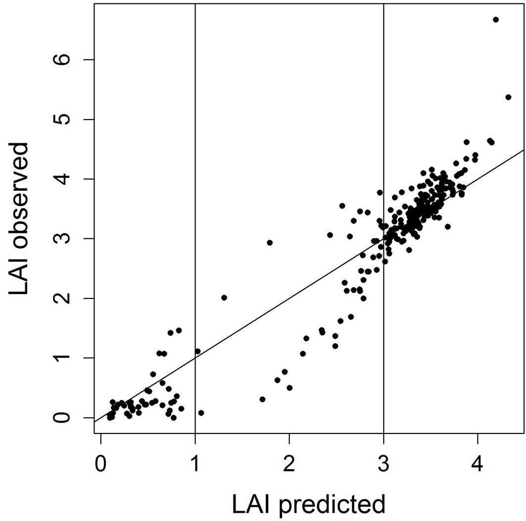
- Exploratory analysis revealed that the model fit is better for low (<1) and high (>3) LAI values than for intermediate ones (Fig. 2). Therefore, the range of predicted LAI values was subdivided into 3 classes and for each class MAE and confidence intervals were calculated.
- An area-weighted MAE was calculated by weighting the MAE of each class with its areal extent.
- To highlight that model fit was not even over the whole range of predicted LAI values a spatial distribution of per class MAE values was presented as a supplementary map (Fig. 7).
- The share of the total image area covered by reflectance values that were beyond the range of training data was stated and the corresponding area mapped.
Fig. 2 - Scatterplot of predicted vs. observed LAI values. The subdivision of predicted LAI values into three classes (<1, 1-3, and >3) according to the fit of the RF model used for predicting LAI is indicated. Prediction accuracy was lowest for the intermediate LAI class (LAI 1-3).
Assessing the influence of texture features on LAI prediction
To evaluate the influence of texture features on LAI predictions, RF models were built either using only VIs, only texture features, or both jointly. Generalization performance of these models was evaluated by the MAE_CV, calculated as described above. Wilcoxon`s rank sum test was applied to test whether differences in MAE_CV were significant at α = 0.05. In this analysis only those VIs and texture features which were classified as relevant by the Boruta analysis were considered.
Results
Response variable
Observed LAI values ranged from 0 to 6.67 with a mean LAI of 2.75. Predicted LAI values covered a smaller range from 0.1 to 4.32 with a mean LAI of 2.74. In the scatterplot depicting observed vs. predicted LAI values (Fig. 2), it is obvious that low LAI values tended to be over-predicted, while high LAI values tended to be under-predicted. Two data points having exceptional high observed LAI values were grossly under-predicted by the RF model. A tendency towards a better model fit for high and low LAI values was visible. For the intermediate section of the LAI range, for which only few observations were available, the accuracy of predictions was lower.
Predictor variables
Based on the Boruta analysis we identified 22 out of the 59 predictor variables as being relevant for predicting LAI. Among these, all 6 VIs were ranked at high positions (Fig. 3), with NDVI-GREEN ranked lowest at 10th position. The VIs using the RED-EDGE bands information, CHLOROPHYLL-RED-EDGE-MODEL (CRM) and NDVI-RED-EDGE, stand out as the top two predictor variables. Interestingly, the RED-EDGE and the NIR bands themselves were ranked distinctly lower at rank 17 and 31, respectively. The RapidEye bands RED, GREEN, and BLUE were listed at positions 9, 11, and 12 of the ranking.
Fig. 3 - Ranking of predictor variables according to their importance assessed by the Boruta algorithm. Boruta generates random variables and tests whether correlations of these random variables with decisions are higher than correlations of real variables with decisions. Colouring: (grey): relevant variables; (white): irrelevant variables. Prefixes: (RE): RapidEye band; (VI): vegetation index; (TX): texture feature. The numbers (3, 5, and 7) following the TX-prefix refer to the moving window size of 15, 25, and 35 m side length, respectively.
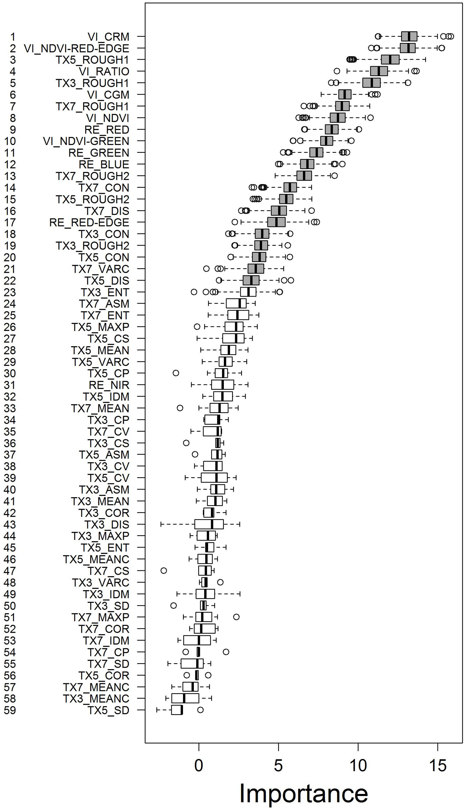
The texture feature ROUGH1 was ranked 3rd, 5th, and 7th for moving window sizes 15, 25, and 35 m side length, respectively. ROUGH2, calculated for all 3 moving window sizes, was ranked among the relevant predictor variables at positions 13, 15, and 19. From the group of co-occurrence texture features only CON, DIS, and VARC were classified relevant. All occurrence texture features were classified irrelevant.
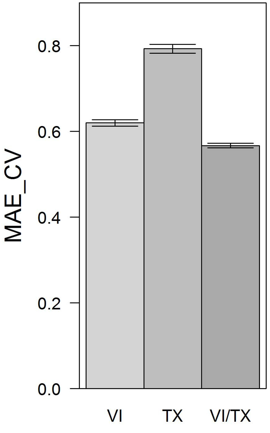
Comparing the MAE_CV values resulting for RF models based on VIs only, texture features only, and VIs and texture features combined, lowest MAE_CV was observed for the RF model based on the combination of VIs and texture features (MAE_CV = 0.57). The RF model based on VIs only was ranked second (MAE_CV = 0.62). The RF model exclusively using texture features performed worst (MAE_CV = 0.79 - Fig. 4). All observed differences were significant.
Fig. 4 - MAE_CV based on 20 repetitions of 10-fold cross validations for RF models using VIs only, texture features only, and VIs and texture features combined. Error bars depict standard deviations of MAE_CV values calculated over 20 repetitions.
Backward selection of variables resulted in MAE_CV values for RF models as depicted in Fig. 5. The lowest MAE_CV = 0.56 was achieved by the RF model using the top 14 predictor variables. Since the MAE_CV of this model was not significantly different from the RF model using only the top 8 predictor variables (MAE_CV = 0.57, p = 0.1) we selected this more parsimonious RF model for predicting/mapping LAI. All MAE_ CV values of RF models using less than 8 predictor variables were significantly different from the MAE_CV of the RF model having the lowest MAE_CV.
Fig. 5 - Backward elimination of predictor variables. Points represent mean MAE_CV (error bars: standard deviation) for RF models based on the respective predictor variable given on the y-axis combined with those listed above that predictor variable.
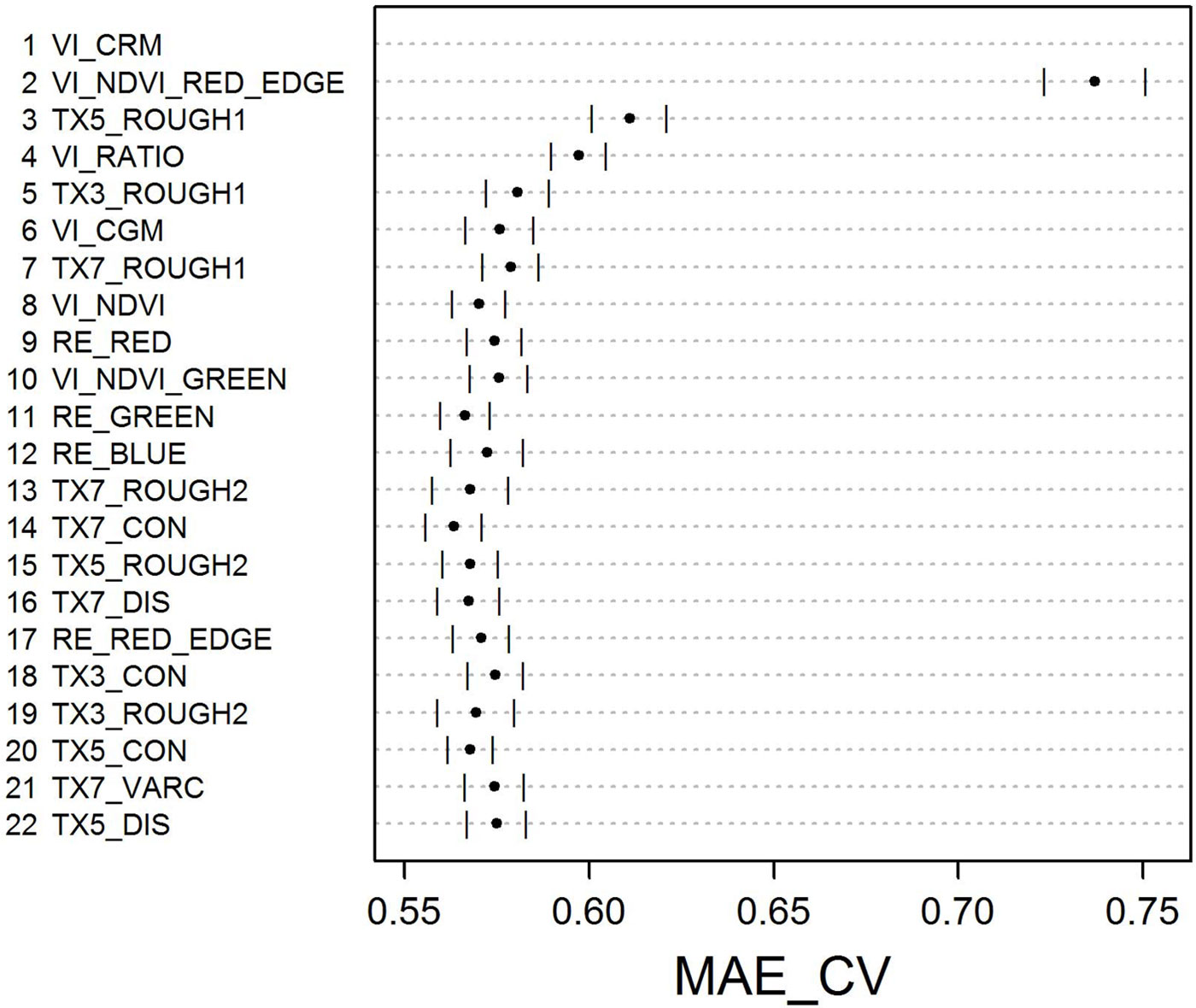
It is worth mentioning that the highest MAE_CV was observed for the RF model using only the top two predictor variables, the VIs CRM and NDVI-RED-EDGE. However, if the texture feature ROUGH1 is included into the RF model, MAE_CV drops considerably (p < 0.0001).
LAI map - spatial prediction of LAI
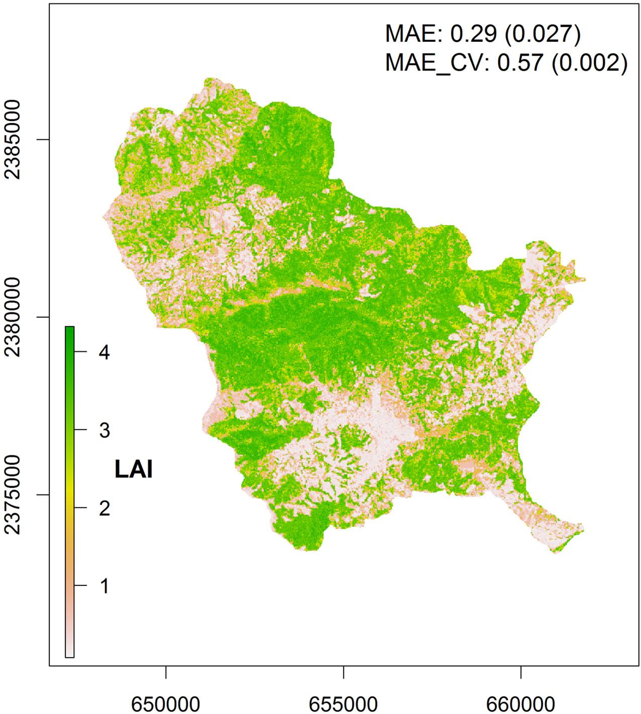
We produced a wall-to-wall LAI map of the study area by applying the selected RF model to the corresponding combination of image features (Fig. 6). MAE_CV of the LAI map was 0.57 and the MAE was 0.29. The area-weighted MAE (0.35) was slightly higher than the unweighted MAE (Tab. 2). This difference occurred because: (1) the MAE of the intermediate LAI class was noticeably higher than the MAE of the other classes; and (2) the intermediate class covered roughly one third (29% - Fig. 7) of the mapping area, thus, its MAE was weighted by a factor of the same magnitude as those of the other two classes (Tab. 2). The larger differences between observed and predicted LAI values occurring in the intermediate LAI class did not influence the unweighted MAE too much since the total number of observations in this class was lower compared to those of the other two classes (Tab. 2).
Fig. 6 - LAI map for the Mensgong study site (January 11, 2011). Map uncertainty was approximated by the MAE and the MAE_CV (complemented with their estimated standard errors - in parenthesis).
Tab. 2 - Mean Absolute Error (MAE) calculated for 3 sections of predicted LAI values.
| LAI section |
No. of observations |
MAE | Area (pixel) |
Weight | Area-weighted MAE | ||||
|---|---|---|---|---|---|---|---|---|---|
| Value | % | SD | SE | Value | SE | ||||
| <1 | 45 | 0.25 | 57.81 | 0.3 | 0.05 | 63913 | 0.27 | 0.07 | 0.01 |
| 1-3 | 43 | 0.65 | 25.93 | 0.71 | 0.11 | 68113 | 0.29 | 0.19 | 0.03 |
| >3 | 164 | 0.21 | 6.07 | 0.3 | 0.02 | 102546 | 0.44 | 0.09 | 0.01 |
Fig. 7 - Map of model fit, quantified by the MAE, as a proxy for prediction uncertainty associated with LAI map (Fig. 6). Overall, 7.46 % of the mapping area were covered by pixel values that were out of range (OOR) of training data. (SE): standard error.
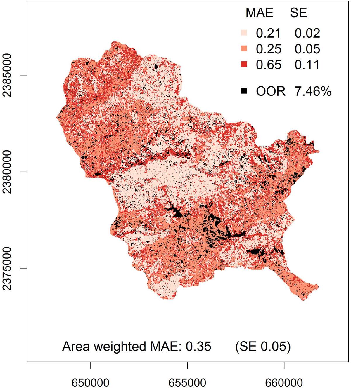
Exploratory analysis of image areas associated with high MAE values revealed that high MAE values cannot be directly related to specific vegetation types. Furthermore, the variability of predictor variables for the corresponding LAI class was not higher than for the other classes (Tab. 3).
Tab. 3 - Coefficient of variation of predictor variables’ pixel values per LAI class standardized by the respective number of observations per LAI class.
| LAI (observed) |
VI_CRM | VI_NDVI- RED-EDGE |
TX5_ ROUGHNES1 |
VI_RATIO | TX3_ ROUGHNES1 |
VI_CGM | TX7_ ROGHNES1 |
VI_NDVI |
|---|---|---|---|---|---|---|---|---|
| <1 | 0.77 | 0.52 | 1.82 | 0.34 | 1.73 | 0.7 | 1.86 | 0.47 |
| 1-3 | 0.53 | 0.33 | 2.29 | 0.26 | 2.21 | 0.55 | 2.13 | 0.22 |
| >3 | 0.09 | 0.05 | 0.34 | 0.03 | 0.37 | 0.13 | 0.33 | 0.03 |
Overall, 7.46% of the study site were covered by pixel values beyond the range of our training data (Fig. 7). Visual inspection revealed that primarily water bodies, settlements/roads, bare agricultural land, and mining claims were represented by these pixel values. Nevertheless, out-of-range pixel values were also found within vegetated areas, yet no vegetation type could be identified as being particularly affected.
Discussion
We produced a high resolution map depicting the spatial variability of LAI by combining RapidEye data and LAI estimates obtained from field sampling. Such map has the potential to be used in spatially distributed modeling of vegetation productivity, evapotranspiration, and surface energy balance ([65], [63]), and it can support a better understanding of ecosystem processes over large and remote areas ([14]). This is particularly important for regions like Xishuangbanna that harbor a high biodiversity ([73], [42]) which is threatened by the dramatic expansion of rubber plantations ([72], [42]). The results from this study provide information to make inferences about ecosystem dynamics of our study area. The presented approach to map LAI using the RF algorithm has the potential to be transferred to other geographical regions harboring different vegetation types. Transferred to another region, the resulting LAI maps presumably carry an error which differs from that reported by our study. Therefore, the user should make sure that map uncertainties are described adequately.
The LAI values observed in this research were slightly lower but generally in accordance with other studies assessing LAI in tropical/ subtropical ecosystems. In a review paper Asner et al. ([2]) reported a mean LAI of 4.9 for tropical evergreen broadleaf forests. Roberts et al. ([55]) obtained LAI values ranging from 4.1 to 8.0 for tropical lowland rainforests, with a tendency for higher values in Asia. Along a gradient covering open pasture, secondary forests, regeneration forests after selective logging, and old-growth forests Tang et al. ([63]) mapped LAI using waveform LIDAR at La Selva, Costa Rica and observed mean values of 1.74, 5.20, 5.41, and 5.62 LAI, respectively. Nevertheless, there are few studies for direct comparisons since different definitions of LAI are frequently used ([3]) and different methods for LAI determination are applied in the field ([9], [2]). Furthermore, a significant fraction of literature on LAI does not describe the methodology used in sufficient detail, thus, comparability is hampered ([2], [7]). Differences between studies may also arise from seasonal changes in LAI due to changes in rainfall volume and other climatic parameters ([9]). In our study, field data and remote sensing data were acquired within the dry season, which might have caused slightly lower LAI values compared to those found in the literature.
Except for two outliers showing observed LAI values distinctly higher than predicted, a good agreement between observed and predicted LAI values was found. MAE was highest for the intermediate LAI class containing lower numbers of observations. Higher MAE values might be explained by the greater spatial variability of LAI values observed in this class resulting from heterogeneous shrub vegetation and trees scattered within grasslands. In such a heterogeneous landscape slight location errors in field and satellite data might result in perceptible prediction errors. Using a pixel size of 20x20 m we tried to account for these errors but in some cases they may still occur. Moreover, it needs to be taken into account that LAI as derived from hemispherical photographs is a modeled value in itself, which might already carry an unknown error. Further, a tendency towards an under-prediction of high LAI values and an over-prediction of low LAI values has been observed. This is because the response from a RF model, in the case of regression, is a value resulting from averaging the predictions made by all trees within a RF ([35]).
VIs derived from RapidEye data, especially those making use of the RED-EDGE band, appeared to be important for predicting LAI. The importance of the RED-EDGE information results from the sensitivity of the respective electromagnetic spectrum (680-740 nm) to vegetation chlorophyll content that shows an abrupt rise in reflectance caused by vegetation. This is related to strong chlorophyll absorption and high internal leaf scattering of plant tissue ([57]). By choosing the RED-EDGE band, instead of the RED band for the NDVI calculation, a lower saturation over highly vegetated area is achieved ([64]). Surprisingly, the RED-EDGE band itself was only ranked 17th among the relevant predictor variables. The higher ranking of VIs might be explained by their general ability to reduce the impacts of confounding factors such as soil reflectance and atmospheric effects on reflectance values ([5], [45]).
Besides VIs, the texture features ROUGH1 and ROUGH2 were ranked high among the relevant predictor variables. MAE_CV of RF models including VIs and texture features jointly was significantly lower than MAE_ CV of RF models exclusively based on VIs. This shows the potential of texture features derived from RapidEye data to improve the quality of LAI maps and to reduce the associated uncertainties. Similar effects of the inclusion of texture features have been reported for IKONOS satellite data ([17]) and airborne CASI imagery ([70]). Nevertheless, most texture features were classified irrelevant by the Boruta analysis in our study, pointing to the difficulty to identify which specific textural characteristic is represented by each of the texture features ([70]). Texture features vary with the characteristics of the landscape under investigation and image types used ([45]), and besides the identification of appropriate texture features, suitable moving window sizes and image bands need to be determined ([15]). Clear guidelines on how to select appropriate texture features are still lacking; hence, the generation of suitable texture features is a challenging task ([45]). In our study, texture features were calculated for the NIR band using three moving window sizes of 15, 25, and 35 m side length. Whether a different set of texture features would be among the relevant predictor variables if calculated for larger moving window sizes or different spectral bands, was not investigated here but should be considered in future mapping efforts. For LAI mapping it might be of particular interest whether texture features calculated for the two VIs identified as being most relevant for predictions would further increase map accuracy.
Using only a reduced set of predictor variables did not substantially enhance the predictive performance of the RF models. This confirms previous studies stating that RF is generally able to deal with large amounts of non-informative or redundant variables ([19], [41]). Nevertheless, reducing the set of predictor variables might reduce computational cost and increase the interpretability of the predictions made by the model ([61]). In our opinion, reducing model complexity and providing map users with understandable descriptions of the methods used to create a map should be an integral part of predictive mapping. Through this, informed assessments of appropriate and inappropriate uses of maps can be made by the user ([21]).
Map interpretation and inference are directly affected by map accuracy. Therefore, users should not rely on maps without associated estimates of error ([12]). Addressing this issue, we provided estimates of data fit and generalization performance of the RF model. Following the recommendation of Mitchard et al. ([47]), we additionally complemented the produced LAI map with an estimated spatial distribution of accuracy. From this map an area weighted MAE was calculated. By providing an area weighted MAE and the corresponding MAE map, the user is able to evaluate the usefulness of the map at hand. Mapping of areas having pixel values which were beyond the range of reflectance values available in the training data appeared to be valuable information. Exploratory analysis revealed that such areas were mainly declared for landscape elements such as water bodies, settlements, or mining areas for which LAI predictions would be questionable.
Our results demonstrate the suitability of RapidEye data to retrieve LAI across a range of landscape classes including forests. Thus, the applicability of RapidEye imagery to deriving LAI for agricultural areas ([64], [68]) can be broadened to include forest ecosystems. This is especially valuable, as forest LAI is regarded as one of the most important structural variables for understanding ecosystem processes ([8]).
Acknowledgments
Our thanks are due to the Advisory Group on International Agricultural Research (BEAF) at the German Agency for International Cooperation (GIZ) and the German Ministry for Economic Cooperation (BMZ) for funding the research project MMC (Making the Mekong Connected, Project No. 08.7860.3-001.00) within which this study had been carried out. We are also grateful to all members of the MMC-project for their support. We acknowledge the German National Space Agency DLR (Deutsches Zentrum für Luft- und Raumfahrt e.V.) for the delivery of RapidEye images as part of the RapidEye Science Archive (Proposal No. 390). The provision of RapidEye images was funded by the German Federal Ministry of Economics and Technology. The responsibility for any use of the results lies with the user. We also thank Mr. Paul Magdon for his support in pre-processing RapidEye images.
References
Gscholar
Gscholar
Gscholar
Gscholar
Gscholar
Gscholar
Gscholar
Gscholar
Gscholar
Gscholar
Gscholar
Gscholar
CrossRef | Gscholar
Gscholar
Gscholar
Gscholar
Gscholar
Gscholar
Gscholar
Gscholar
Gscholar
Authors’ Info
Authors’ Affiliation
Lutz Fehrmann
Christoph Kleinn
Chair of Forest Inventory and Remote Sensing, Georg-August-Universität Göttingen, Büsgenweg 5, D-37077 Göttingen (Germany)
Key Laboratory for Tropical Forest Ecology, Xishuangbanna Tropical Botanical Garden, Chinese Academy of Sciences, Menglun, Mengla, 666303 Yunnan (China)
World Agroforestry Centre, ICRAF-Kunming Office, Kunming, 650201 Yunnan (China)
Corresponding author
Paper Info
Citation
Beckschäfer P, Fehrmann L, Harrison RD, Xu J, Kleinn C (2014). Mapping Leaf Area Index in subtropical upland ecosystems using RapidEye imagery and the randomForest algorithm. iForest 7: 1-11. - doi: 10.3832/ifor0968-006
Academic Editor
Giorgio Matteucci
Paper history
Received: Feb 06, 2013
Accepted: May 13, 2013
First online: Oct 07, 2013
Publication Date: Feb 03, 2014
Publication Time: 4.90 months
Copyright Information
© SISEF - The Italian Society of Silviculture and Forest Ecology 2014
Open Access
This article is distributed under the terms of the Creative Commons Attribution-Non Commercial 4.0 International (https://creativecommons.org/licenses/by-nc/4.0/), which permits unrestricted use, distribution, and reproduction in any medium, provided you give appropriate credit to the original author(s) and the source, provide a link to the Creative Commons license, and indicate if changes were made.

Web Metrics
Breakdown by View Type
Article Usage
Total Article Views: 64006
(from publication date up to now)
Breakdown by View Type
HTML Page Views: 51091
Abstract Page Views: 4525
PDF Downloads: 6381
Citation/Reference Downloads: 42
XML Downloads: 1967
Web Metrics
Days since publication: 4650
Overall contacts: 64006
Avg. contacts per week: 96.35
Article Citations
Article citations are based on data periodically collected from the Clarivate Web of Science web site
(last update: Mar 2025)
Total number of cites (since 2014): 23
Average cites per year: 1.77
Publication Metrics
by Dimensions ©
Articles citing this article
List of the papers citing this article based on CrossRef Cited-by.
Related Contents
iForest Similar Articles
Review Papers
Digital hemispherical photography for estimating forest canopy properties: current controversies and opportunities
vol. 5, pp. 290-295 (online: 17 December 2012)
Review Papers
Remote sensing-supported vegetation parameters for regional climate models: a brief review
vol. 3, pp. 98-101 (online: 15 July 2010)
Research Articles
Remote sensing of Japanese beech forest decline using an improved Temperature Vegetation Dryness Index (iTVDI)
vol. 4, pp. 195-199 (online: 03 November 2011)
Research Articles
Estimation of forest leaf area index using satellite multispectral and synthetic aperture radar data in Iran
vol. 14, pp. 278-284 (online: 29 May 2021)
Research Articles
The estimation of canopy attributes from digital cover photography by two different image analysis methods
vol. 7, pp. 255-259 (online: 26 March 2014)
Research Articles
Mapping the vegetation and spatial dynamics of Sinharaja tropical rain forest incorporating NASA’s GEDI spaceborne LiDAR data and multispectral satellite images
vol. 18, pp. 45-53 (online: 01 April 2025)
Review Papers
Accuracy of determining specific parameters of the urban forest using remote sensing
vol. 12, pp. 498-510 (online: 02 December 2019)
Short Communications
Estimation of canopy attributes of wild cacao trees using digital cover photography and machine learning algorithms
vol. 14, pp. 517-521 (online: 17 November 2021)
Research Articles
Assessing the influence of different Synthetic Aperture Radar parameters and Digital Elevation Model layers combined with optical data on the identification of argan forest in Essaouira region, Morocco
vol. 17, pp. 100-108 (online: 24 April 2024)
Research Articles
Evaluation and correction of optically derived leaf area index in different temperate forests
vol. 9, pp. 55-62 (online: 11 June 2015)
iForest Database Search
Google Scholar Search
Citing Articles
Search By Author
Search By Keywords


