The missing part of the past, current, and future distribution model of Quercus ilex L.: the eastern edge
iForest - Biogeosciences and Forestry, Volume 17, Issue 2, Pages 90-99 (2024)
doi: https://doi.org/10.3832/ifor4350-016
Published: Mar 22, 2024 - Copyright © 2024 SISEF
Research Articles
Abstract
Ongoing climate change is anticipated to shift the geographical distribution range and impact local abundance of tree species by altering their ecological conditions. Given the lower resilience of populations at the species’ range edges, locally adapted range-edge populations are critical to the species’ survival under climate change. In this context, the distribution of holm oak (Quercus ilex L.) at the eastern border of its distribution range was assessed under current, past, and foreseeable future climate change scenarios, using species distribution models (SDMs). Current SDMs were developed using WorldClim 1.4 climate data as baseline at 30-second spatial resolution by using Generalized Boosted Regression Models (GBM) and showed moderate model performance. To compare temporal transferability and account for climate uncertainties of two versions of future climate data (CMIP5 and CMIP6), we used 4 Global Circulation Models (GCMs), 2 emission scenarios (moderate RCP45/SSP245 and pessimistic - RCP85/SSP585) for 2 different periods in the future (2040-2060 and 2060-2080). We also made predictions about the past (Mid-Holocene, about 6.000 years ago) using 4 CMIP5 GCMs. Most important variables of SDMs were distance to the sea, isothermality (BIO3), annual precipitation (BIO12), the mean temperature of driest quarter (BIO9), and the precipitation of driest month (BIO14). Our findings showed that the species’ potential distribution range probably used to be much wider in the mid-Holocene, which implies that the holm oak had a broader climatic niche during this period. The future projections indicate that its distribution area in the eastern border might increase particularly in the Black Sea region, while decreasing in the Aegean region resulting in a likely northward range shift in Turkey. However, other variables not included in our models such as land use changes might drive future shifts. Due to its high resistance to dry conditions and resilience, this species might continue to spread in southwestern Turkey in 2050s and 2070s. Finally, our study fills the gap in potential distribution predictions in context of climate change for the eastern boundary of the holm oak.
Keywords
Species Distribution Model, Global Circulation Models, Holm Oak, Turkey, Range Edge, Generalized Boosted Regression Models, Climate Change
Introduction
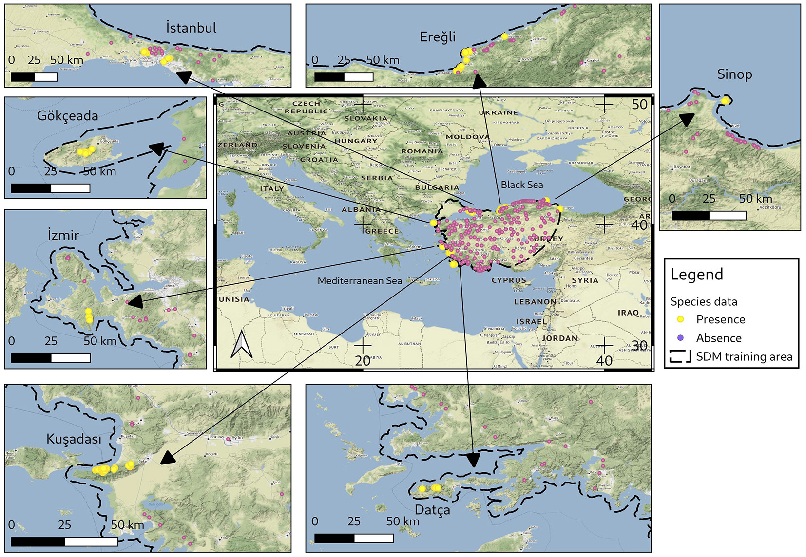
Quercus ilex L., commonly known as holm oak (or holly oak), is an evergreen broadleaved small to medium-sized tree or shrub that is characterized by dark green leathery leaves with a wooly lower side, and acorns which mature in one year. Holm oak acorns are dispersed by animals, especially the Eurasian jay (Garrulus glandarius L.) and rodents ([23]). The tree is usually distributed in the Mediterranean area and is widely accepted as a Mediterranean element, but it also grows in the Black Sea and Aegean regions in Anatolia, in Morocco ([7]), Northern Italy and France ([14]), and appears scattered along Africa’s Libyan coast ([54]). Holm oak, which is highly adaptable to different environmental conditions, various soil types, and a wide variety of climatic conditions, forms pure stands or mixed stands in the Mediterranean basin ([14]). In Turkey, which is the easternmost border of its distribution in the world, it has a limited distribution that is discontinuous and fragmented. The holm oak populations, some of which are remarkably restricted, occur in few widely separated localities near the seaside in the Black Sea and Aegean regions (Fig. 1). These populations do not penetrate into the inner parts of Anatolia but are rather found close to the sea ([2]). Although the species is present as a maquis element at high elevations, it is found as middle-sized trees in pure or mixed forests in humid regions throughout the Marmara and Western Black Sea Regions of Turkey ([3]).
Fig. 1 - Current main distribution sites and occurrences of the holm oak in Turkey. Yellow points represent the species’ presences, pink points represent the species’ absence. The training area used in SDMs is the polygonal area drawn with a black line.
Knowing the current ranges of forest tree species and predicting trajectories of change of their distribution in the upcoming period is valuable to reduce the negative impact of climate change on forest ecosystems ([20], [34], [26]). Understanding how trees can change their distribution in response to ongoing climate change is crucial to ensure the sustainable management of the species and forests, especially for tree species distributed in fragmented populations far from each other or near the borders of their range. Although forest tree species have the ability to respond and adapt to future climatic conditions, management strategies such as assisted migration should be used as a conservation option in response to predicted climate change for the sustainable management of forest communities, especially for fragmented forests ([32]).
In the Mediterranean basin, which has a rich species diversity and high endemism rate, ongoing climate change negatively impacts biodiversity through loss of species. Further, the loss of species in this region can translate into greater loss in terms of global biodiversity ([40]). Climate change, particularly in the Mediterranean basin, is predicted to shift the natural distribution range of tree species because it alters their ecological conditions ([52]). The shift due to climate change will be more evident at the species’ range edges as edge populations are more affected by habitat changes than the ones in the center (the range edge effect sensu [6]). The range-edge populations have a critical role in persisting and expanding their species distributions in the rapid ongoing climate change ([50]). These populations are also important for biodiversity conservation, especially rear-edge populations which are confined to small and isolated habitat islands, are more prone to extinction and thus are of particular importance for conservation ([28], [45]).
Species distribution models (SDMs) predict the potential distribution areas of the species by using the known distribution of the species in a given region and the habitat conditions of the species ([18]). They are also used to simulate future habitat suitability of the species ([26], [17]) to assist managing forests ([10]), and to support conservation decisions (e.g., preventing biological invasions, targeting monitoring and conservation in areas of potential future occupancy, assisted migration, targeting other species with positive interactions - [25]) in the context of global climate change. Since the correlative species distribution models utilize the statistical relationship between spatial environmental variables and species presence-absence data to find indirect factors that limit the distribution of species, they make ecologically realistic predictions ([26]). Presence and absence data required for these models can be collected via field expeditions, observations made by citizen scientists, sensor networks, or they can be obtained from herbarium records, atlases, large databases such as national or regional inventories.
Under the effect of climate change, climate in the Mediterranean region is projected to be warmer and drier ([22]), and the distribution of Mediterranean oak forests could be affected in a complex way ([1], [37], [36]). Cheaib et al. ([12]) forecasted that the Mediterranean broadleaved evergreen species (including holm oak) would significantly expand their distribution across western France. For these species, vast range expansions have been forecasted by their models, but estimates for the size and location of the changes are highly varied. Since model uncertainties stemming from factors such as spatial biases, model fitting algorithms and parameters, and choice of predictors lead to wide variations in predictions of the rate and direction of migration under the influence of climate change, it is not certain that many of these species will actually be able to achieve such rapid migration ([17]). Interpreting their current and future projections produced by taking Topographic Wetness Index (TWI) into account, Petroselli et al. ([44]) found that the holm oak is expected to increase its distribution area in the future. They stated that among the evergreen oak species found in the Mediterranean basin, holm oak has one of the highest tolerances to extreme summer temperatures and water scarcity.
The current distribution range of the species ([14]) and also its future potential distribution are known in the Mediterranean Basin and Europe because several studies have been conducted around Europe, where the species is mainly distributed ([5], [12], [15], [36], [38], [21]). However, regarding Turkey, current distribution of the species is not fully known since it is indicated only as Oak in the forest management plans. Further, in the context of global climate change, future distribution projections of the species in Turkey are also lacking. It is crucial to know the possible effects of climate change on the distribution of the species at the range limits, because in these regions there may be a more pronounced effect as the growing conditions are usually close to the tolerance limits of the species ([13]).
Due to the holm oak’s crucial importance for forest management and urban greening, its distribution area at current and in the future should be identified. Hence, the purpose of the study is to model the potential distribution of holm oak in response to climate change, in several time periods of the past (Mid-Holocene, about 6.000 years ago), current (1960-1990), and future (2050s, 2070s). Using a machine learning approach, we investigated the actual and potential distribution of holm oak at the eastern edge of the species’ where this information was previously missing. The aims of this investigation were (i) to predict the current potential distribution of the species, (ii) to predict potential mid-Holocene distribution and compare it with current distribution, and (iii) to forecast its potential distribution according to different future climate change scenarios.
Materials and methods
Study area and species data
The study covers all known distribution areas in the Black Sea, Marmara, and Aegean regions in Turkey, which form the eastern range edge of the holm oak (Fig. 1). The study area is characterized by considerable climatic, topographical, and geological variability, including the humid areas in the northern and northwestern parts, and the semi dry and semi humid areas in the western and southern parts of Turkey. During field studies, it was observed that except for well-developed populations within protected areas, the species’ habitats have been severely altered and contracted due to land use change. These destroyed areas have been transformed into hazelnut groves in the Black Sea region and olive groves in the Aegean region. In addition, since the species is located on the coastline, some of these areas have been developed into residential ar-eas or summer residences ([2]). This situation makes it necessary to focus on the locations where the species could exist but no occurences were found. During field works for this study, two new distribution areas (one in Datça, and one in Izmir) were discovered ([3]). Unlike its general distribution in the Mediterranean, the species appears almost like a rare species in Turkey due to its current limited distribution.
It is known that the species is distributed in 7 main regions where it forms forest stands in Turkey (Fig. 1). The distances between these regions range from 100 to 300 km. In these regions, the minimum area covered by the distribution of the species is about 50 ha and the largest area is about 2500 ha. Except for herbarium records and some academic studies ([27], [2]), there is no information on the distributions of the species in Turkey.
Location of 21 different holm oak records in the ISTO Herbarium were selected to be used as the “presence” data. Upon field examinations to verify the locations of these points, 16 of them were taken as presence data. In addition, within the scope of the study on holm oak ([2]), 102 sample plots (20 × 10 m quadrat) taken from 7 known distribution regions were added as presence data. In most of the sampling plots, holm oak is the dominant tree species except for plots that have old Pinus brutia Ten. individuals. Potential presence areas of the species were visited during the field trips for this study. Combining the verified locations from the records of ISTO Herbarium (16 verified locations) with the species found in these sampling plots (102 sampling plots), a total of 118 presence locations were obtained. A total of 210 locations where the species could not be found were recorded as absence data. The geographical coordinates of all the presence-absence locations collected in the field were recorded with the mobile phone GNSS with the accuracy of <5 m.
During this process of recording presence and absence data, potential locations of the species in anthropogenically damaged and affected areas - urbanized or changed vegetation type to olive (Olea europaea L.) or hazelnut (Corylus avellana L.) planted areas - were not taken into account. Since it is known that the holm oak tree in Turkey does not spread very far from the coastal areas, an additional 90 randomly assigned absence locations to the area at least 170 km from the coast (inner Anatolia) were added to the absence data. In order to minimize spatial autocorrelation, points within 1 km of each other were eliminated which reduced the presence locations from 118 to 75 and absence locations from 300 to 286. The species’ dispersed and discontinuous distribution in Turkey is the main reason for the prevalence of absence data over presence data. Background data was not used because the accuracy of the presence data in terms of spatial and species identification as well as the accuracy of the absence data affects the success of the model ([9]).
The extent of the study region affects the model results ([4]). Therefore, a polygon area covering all the presence-absence data of the species was created as a “minimum enclosing circle area” and used for current, past, and future distribution estimates in model calibration and projection (Fig. 1). We used QGIS software ([48]) for the preparation of species data.
Environmental variables
In this study, we used 19 bioclimatic variables (Tab. 1), which are widely used in species distribution models, and the “distance to sea” variable as environmental data. The "distance to sea" variable was selected for inclusion due to the experiences gained in field observations and iterative modeling experiments. We used WorldClim 1.4 climate data (1960-1990) as the current baseline. In order to reveal the change in the future distribution of the species, we used four general circulation models (GCMs) for each version of the climate data, which are HadGEM2-ES, IPSL-CM5A-LR, MIROC5 and MPI-ESM-LR for WorldClim 1.4 and HadGEM3-GC31-LL, IPSL-CM6A-LR, MIROC6 and MPI-ESM1-2-LR, for WorldClim 2.1. We considered projections to the 2050s (2040-2060) and 2070s (2060-2080) periods and two emissions scenarios from the four available GCMs. The Representative Concentration Pathways (RCPs) RCP4.5 and RCP8.5 were selected for the CMIP5 (downscaled and calibrated with WorldClim v1.4). For the CMIP6 (downscaled and calibrated with WorldClim v2.1), SSP245 and SSP585 Shared Socio-economic Pathways (SSPs) were used. The purpose of using two different datasets is to reveal potential differences between projections using CMIP5 and CMIP6, as well as the impact of climatic uncertainty and data quality. We also projected the model under past climate conditions in the Mid-Holocene using the four CMIP5 GCMs (HadGEM2-ES, IPSL-CM5A-LR, MIROC-ESM, MPI-ESM-P). After all data was downloaded from the WorldClim website ([30], [19]) with a spatial resolution of 30 arc seconds, the layers were preprocessed (i.e., clipping, masking, stacking) for their use in SDM creation ([31]).
Tab. 1 - The correlation coefficients between the selected variables affecting the distribution of the species (WC14) and the bioclimatic variables of WorldClim 1.4 Data. (*): P<0.05.
| - | BIO3 | BIO9 | BIO12 | BIO14 | Description |
|---|---|---|---|---|---|
| BIO1 | - | 0.97* | - | - | Annual Mean Temperature |
| BIO2 | 0.75* | - | - | - | Mean Diurnal Range |
| BIO3 | - | - | - | - | Isothermality |
| BIO4 | - | - | - | - | Temperature Seasonality |
| BIO5 | - | 0.92* | - | - | Max Temperature of Warmest Month |
| BIO6 | - | 0.88* | - | - | Min Temperature of Coldest Month |
| BIO7 | - | - | - | - | Temperature Annual Range |
| BIO8 | - | - | - | - | Mean Temperature of Wettest Quarter |
| BIO9 | 0.42 | - | - | - | Mean Temperature of Driest Quarter |
| BIO10 | - | 0.99* | - | - | Mean Temperature of Warmest Quarter |
| BIO11 | - | 0.92* | - | - | Mean Temperature of Coldest Quarter |
| BIO12 | -0.09 | 0.32 | - | - | Annual Precipitation |
| BIO13 | - | - | 0.90* | - | Precipitation of Wettest Month |
| BIO14 | -0.48 | -0.34 | 0.36 | - | Precipitation of Driest Month |
| BIO15 | - | - | - | - | Precipitation Seasonality |
| BIO16 | - | - | 0.91* | - | Precipitation of Wettest Quarter |
| BIO17 | - | - | - | 0.99* | Precipitation of Driest Quarter |
| BIO18 | - | - | - | 0.98* | Precipitation of Warmest Quarter |
| BIO19 | - | - | 0.88* | - | Precipitation of Coldest Quarter |
Species distribution modeling and performance
For the species distribution modeling of the holm oak tree, we used R software v. 4.2.1 (23.06.2022) “Funny-Looking Kid” ([49]) installed on a virtual computer (Intel® Xeon® Gold 6238R processor x16 cores, 32 GB memory) with Ubuntu 22.04.1 LTS operating system. Throughout the data processing steps, for the creation of models, and postprocessing of SDMs outputs, the R packages “biomod2 v. 4.2-4” ([57]), “terra” ([31]), “sf” ([43]), “usdm” ([39]), “ggplot2” ([59]), and “doParallel” were used in the R environment. Species distribution models were created by using holm oak presence-true absence data and environmental variables. At this stage, we tested the algorithms commonly used in species distribution modeling included in the biomod2 package (“GLM”, “GBM”, “GAM”, “CTA”, “ANN”, “SRE”, “FDA”, “MARS”, “RF”, “MAXENT.Phillips”, and “XGBOOST”). We employed Generalized Boosted Regression Models (GBM) algorithms that gave the best and the highest accuracy scores. Since the “Maxent” model works better with “presence only (with pseudo-absence)” data ([46]), this algorithm was not successful in the pre-test due to the use of presence-true absence data in our study. Layers showing multicollinearity among the environmental data were excluded by using the “variable inflation factor” (VIF) method ([39]) and the remaining six bioclimatic layers (Isothermality-BIO3, Temperature Seasonality-BIO4, Mean Temperature of Wettest Quarter-BIO8, Mean Temperature of Driest Quarter-BIO9, Annual Precipitation-BIO12, Precipitation of Driest Month-BIO14) and distance to the sea were used in the models.
The Generalized Boosted Regression Models (GBM) used in the study is a machine learning method and has important advantages for tree-based algorithms. We used the “gbm” package ([24]) from the R statistical environment which uses the aforementioned algorithm for fitting the models, assessing relative contributions, making predictions, and mapping distribution. To prevent overfitting and determining user-defined parameters, the “biomod2” package includes a function (“BIOMOD_Tuning”) to define the optimum model parameters. Based on tuning results, we selected 0.5 for bag fraction, 7 for interaction depth, 5 for n.minobsinnode, 0.05 for shrinkage and 750 for n.trees. Subsequently, for spatial cross-validation of species data, we tested “block”, “strat”, and “user-defined” cross-validation strategies of biomod2 and decided to use the “block” strategy. The SDM was built with tuned parameters and spatially cross-validated species data. Upon calculating the importance of the variables, two bioclimatic variables with low contribution levels were excluded in the final model. To avoid confusion, the dataset containing selected climate variables will be referred to as “Wc14” for WorldClim version 1.4 and “Wc21” for WorldClim version 2.1. The data set containing these four climate variables and the distance to the sea variable will be referred to as “env14” and “env21” in a similar way.
We evaluated the performance of GBM algorithm with area under the receiver operating characteristic curve (AUC) and true skill statistics (TSS) with validation data. AUC is calculated from the receiver operating characteristic (ROC) plot that gives the false-positive error rate and the true positive rate. TSS takes into account both omission and commission errors, and success as a result of random guessing. Internal biomod2 function which maximizes the TSS score was used to convert continuous values into binary ones. After the model performance and the importance of the variables were determined again, the current distribution maps of the species were created for spatially cross-validated 4 replications by projecting the model to the area covered by the minimum enclosing circle (i.e., training area - Fig. 1). These four spatially cross-validated current model outputs were used for ensemble modeling of current distribution. Afterwards, projections for the selected GCMs and emission scenarios were generated for each climate data version (4 models × 2 scenarios × 2 time periods × 2 climate data version = total 32 projections) using the “BIOMOD_EnsembleForecasting” function of biomod2. In addition, the paleo distribution (Mid-Holocene) of holm oak based on the WorldClim 1.4 baseline (as paleo data for WorldClim 2.1 has not yet been published) were also projected (4 models × 1 scenario × 1 time period × 1 climate data version = total 4 projections) using ensemble hindcasting.
By comparing these future and past distribution projections with the current distribution projection of the species, the “distribution range size change” areas of the holm oak were calculated with the “BIOMOD_RangeSize” function of biomod2 and their maps were plotted. According to the future/past ensemble SDMs, the percentages of loss (PercLoss) and gain (PercGain) of the species were calculated compared to the current ensemble SDM. To create reproducible results, we used seed value where applicable to guarantee that the same results are produced each time we run the code.
Results
Model evaluation and variable contribution
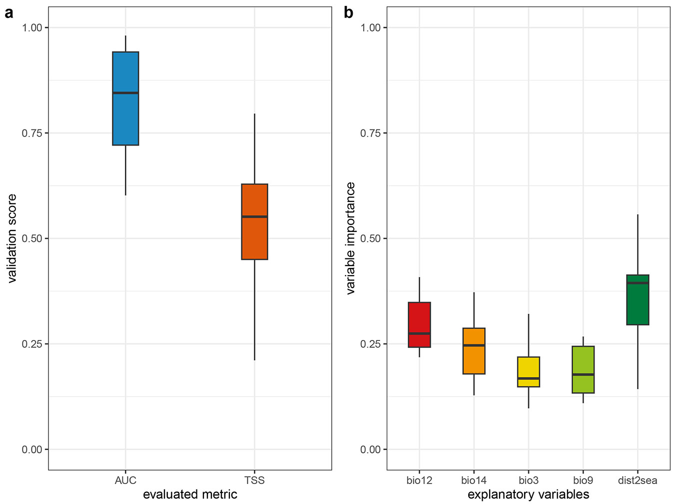
The selected climate variables, resulting from a two-step procedure, are listed in Tab. 1along with their correlations with other climatic variables. Since the correlative species distribution model is based on a statistical relationship between environmental variables and species data, the variables used to model the distribution of the species may be obscuring the true variable as a result of the method followed in the reduction and selection of variables ([16], [55]). Therefore, to strengthen the case for causality, consideration must be given to the correlations between the variables affecting the distribution of the species (Tab. 1). Since some of the variables had very little effect, they were removed and a final model was calibrated using five variables. The distance to the sea, isothermality (BIO3), mean temperature of driest quarter (BIO9), annual precipitation (BIO12), and precipitation of driest month (BIO14) made the most important contributions to the SDMs (Fig. S1 in Supplementary material). Four spatially cross-validated SDMs, with average AUC and TSS values of 0.82 and 0.54 (Fig. 2a), respectively, showed moderate model performance ([20]). While distance to sea was the most important predictor for current model, the least important variable was the mean temperature of driest quarter (BIO9 - Fig. 2b). The optimal isothermality (BIO3) was approximately 0.30 for the probability of presence (Fig. S2 in Supplementary material). The response curve for the mean temperature of driest quarter (BIO9) showed that 21 to 24 °C was suitable for holm oak. Based on the response curve for precipitation during the driest month (BIO14), the suitable precipitation in the driest month was approximately under 20 mm, which further confirmed that holm oak is drought resistant.
Fig. 2 - (a) Model performance of Generalized Boosted Model (GBM) with the validation data calculated using two different performance metrics (TSS, True Skill Statistics; ROC, Receiver Operating Characteristics). (b) Variable contributions used in the models constructed with Generalized Boosted Model (GBM) method.
Current, past and future projections of holm oak distributions
Current distributions
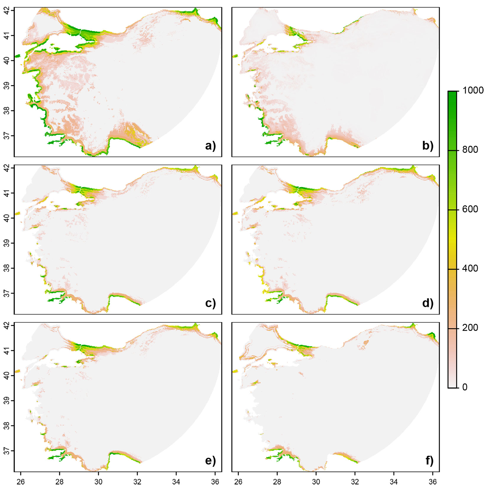
Initial modeling using presence-true absence records and current environmental conditions revealed where current suitable habitats for holm oak are. The result of the current projection for env14 suggested that the suitable habitats for holm oak are mainly located in areas close to the coasts in Black Sea, Marmara, and Aegean regions of Turkey. This was compared with the known distribution of species in order to determine if the models are ecologically plausible. The projected current distribution of the species is close to the real situation observed in the field. However, certain areas, where the species is not currently present due to degradations, were predicted to be part of the potential habitat by the projections. Overall, the model’s performance was considered to be acceptable (Fig. 3).
Fig. 3 - Holm oak training area projections. (a) Past projections; (b) current distribution projections; (c) 2050s RCP45 projections for CMIP5; (d) 2050s RCP85 projections for CMIP5; (e) 2070s RCP45 projections for CMIP5; (f) 2070s RCP85 projections for CMIP5.
Past distributions
The past (mid Holocene), current, and future potential distribution of holm oak under the selected global climate change scenarios for the 2050s (2040-2060) and the 2070s (2060-2080) are displayed in Fig. 3and Fig. S3 (Supplementary material). The projection of the current suitable climatic range of holm oak compared to the Mid Holocene indicates an average reduction of more than 367% in the availability of suitable ranges (i.e., range gain) for env14 (Fig. 4).
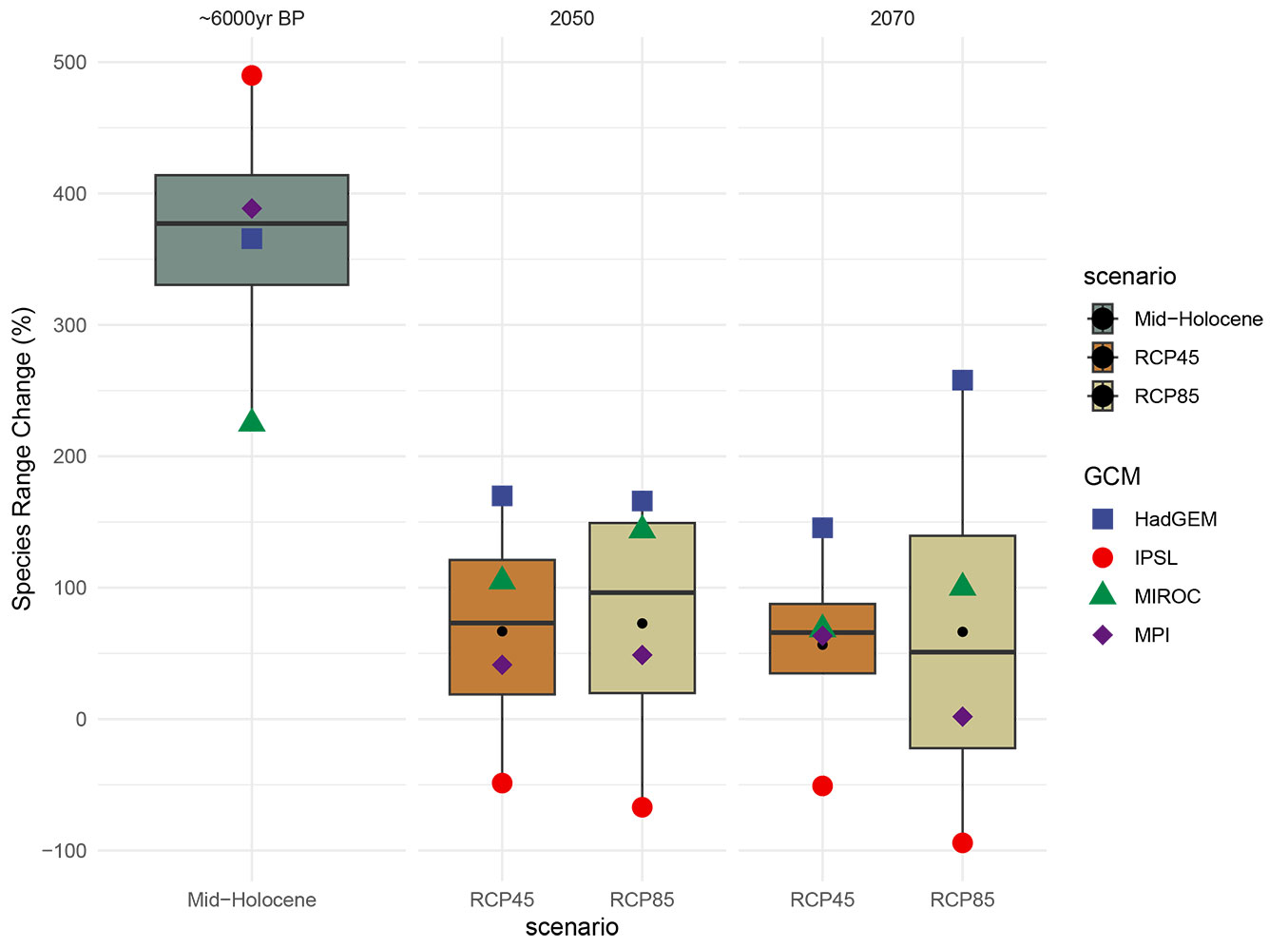
Fig. 4 - Projected species range changes in distribution areas in the mid Holocene period (~6.000 years ago) and 2050s-2070s (percentage of per pixel of holm oak) of Turkey, according to WorldClim 1.4 baseline and CMIP5 paleoclimate and future scenarios.
Future projections of CMIP5 and CMIP6
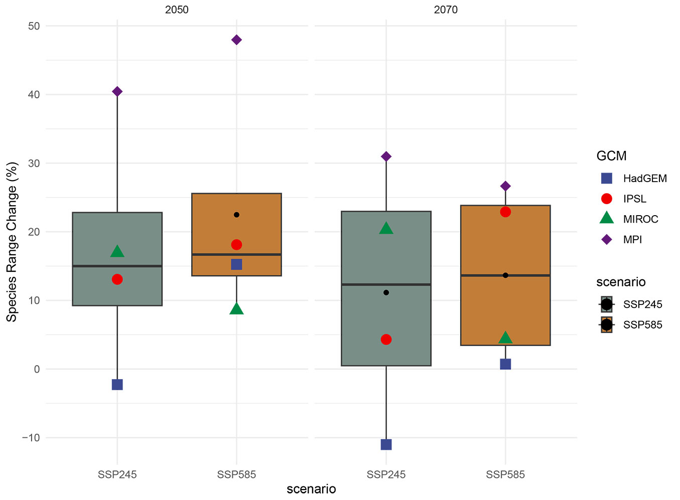
The projections of habitat suitability for holm oak under future climate conditions varied depending on the climate data version, GCMs, and RCPs/SSPs used (Fig. 4, Fig. 5). To understand the internal range shifts of holm oak, we partitioned the total range changes into two components: range loss (PercLoss) and range gain (PercGain - see Tab. S2 in Supplementary material). When the two different climate dataset versions are evaluated in general, the difference in SRC between GCMs is large in CMIP5, but is small in CMIP6. Since CMIP6 is newer than CMIP5, CMIP6 GCMs make estimates that are closer to each other (Fig. 4, Fig. 5). CMIP6 GCMs were generally much higher in species loss than CMIP5 GCMs across all scenarios and periods, but species gain was much lower. Although significant range loss and gain have been observed in holm oak, its average total range change was about 20% in 2050 and 12% in 2070 for CMIP6 and 70% in 2050 and 62% in 2070 for CMIP5, which may reflect obvious range shifting between current and future scenarios (Fig. 4, Fig. 5). The discrepancy between CMIP5 and CMIP6 is also evident, although this might be attributed to the species’ limited range size. Based on future projections obtained using the HadGEM, IPSL, MIROC, and MPI GCMs, average SRC rates in the 2050s were calculated to be 168%, -58%, 124%, and 45% for CMIP5 and 7%, 16%, 13%, and 44% for CMIP6, respectively. In the 2070s, CMIP5 and CMIP6 the average SRC rates from the same GCMs for were 202%, -73%, 84%, and 33%, and -5% for CMIP5 and 14%, 12%, and 29% for CMIP6, respectively. In the 2050 CMIP5 and CMIP6 ensembles, the average SRC rates for the HadGEM, IPSL, MIROC, and MPI GCMs were 168%, -58%, 124%, and 45%, and 7%, 16%, 13%, and 44%, respectively. In the 2070 CMIP5 and CMIP6 ensembles, the average SRC rates for the same GCMs were 202%, -73%, 84%, and 33%, and -5%, 14%, 12%, and 29%, respectively. The average SRC rates in the 2050 for HadGEM, IPSL, MIROC, and MPI GCMs were respectively 168%, -58%, 124%, and 45% for CMIP5 and 7%, 16%, 13%, and 44% for CMIP6. While for the 2070 the average SRC for HadGEM, IPSL, MIROC, and MPI GCMs were respectively 202%, -73%, 84%, and 33% for CMIP5 and -5%, 14%, 12%, and 29% for CMIP6. In contrast to CMIP5, HadGEM GCMs showed the least gain among CMIP6 GCMs in both periods and scenarios. The highest gain for CMIP6 GCMs were returned by MPI GCMs in both periods and scenarios.
Fig. 5 - Projected changes in distribution areas of holm oak in the 2050s and 2070s of Turkey (as %), according to WorldClim14 baseline and CMIP6 climate scenarios.
According to the future projections obtained by using CMIP5 GCMs, it is projected that the distribution area of the species will expand in both periods (2050s and 2070s) and in both scenarios (RCP45 and RCP85). The average change ratio in GCMs is 67% for RCP45 and 72% for RCP85 in 2050s, while in 2070s this ratio is 57% for RCP45 and 66% for RCP85 (Fig. 4). Although considerable range loss and gain have been observed for holm oak, its average total range change was more than 55%, which may reflect obvious range shifting between current and future projections (Fig. 4). The range loss results showed slight differences between GCMs, RCPs, and periods whereas range gain had considerable differences (Tab. 2). According to the IPSL model, it is projected that the distribution area of the species will narrow in both periods and scenarios. (Fig. 4). Among the CMIP5 GCMs, in both periods and scenarios, HadGEM GCMs generally resulted in the highest gain whereas the IPSL model returned the lowest gain. The areas with the highest projected changes in the percentage of species loss by 2070s were mostly located in the south part of Turkey whereas the highest projected changes in the percentage of species gain were mostly located in the north part of Turkey (Fig. 3).
Tab. 2 - Holm oak distribution range change in the past and future projections compared the current distribution projection.
| Version | GCM | Period | Scenario | PercLoss | PercGain | SRC | Loss_ha | Stable0_ha | Stable1_ha | Gain_ha |
|---|---|---|---|---|---|---|---|---|---|---|
| wc14 | HadGEM | 2050 | RCP45 | 9 | 179 | 170 | 60945 | 38314167 | 587802 | 1136473 |
| wc14 | HadGEM | 2050 | RCP85 | 13 | 179 | 166 | 85427 | 38317356 | 563320 | 1133284 |
| wc14 | HadGEM | 2070 | RCP45 | 13 | 158 | 146 | 83053 | 38451468 | 565694 | 999172 |
| wc14 | HadGEM | 2070 | RCP85 | 15 | 273 | 258 | 99307 | 37726098 | 549440 | 1724542 |
| wc14 | IPSL | 2050 | RCP45 | 66 | 17 | -49 | 426016 | 39340691 | 222732 | 109949 |
| wc14 | IPSL | 2050 | RCP85 | 88 | 21 | -67 | 571988 | 39317244 | 76760 | 133395 |
| wc14 | IPSL | 2070 | RCP45 | 70 | 19 | -51 | 453131 | 39328168 | 195617 | 122472 |
| wc14 | IPSL | 2070 | RCP85 | 98 | 4 | -94 | 637037 | 39425464 | 11710 | 25176 |
| wc14 | MIROC | 2050 | RCP45 | 18 | 123 | 105 | 114669 | 38673169 | 534078 | 777471 |
| wc14 | MIROC | 2050 | RCP85 | 12 | 156 | 144 | 80453 | 38461790 | 568294 | 988849 |
| wc14 | MIROC | 2070 | RCP45 | 44 | 112 | 68 | 281817 | 38740087 | 366930 | 710553 |
| wc14 | MIROC | 2070 | RCP85 | 41 | 141 | 100 | 268807 | 38552847 | 379940 | 897793 |
| wc14 | MPI | 2050 | RCP45 | 48 | 89 | 41 | 307381 | 38885382 | 341366 | 565258 |
| wc14 | MPI | 2050 | RCP85 | 61 | 110 | 49 | 398104 | 38750610 | 250644 | 700030 |
| wc14 | MPI | 2070 | RCP45 | 49 | 112 | 63 | 316658 | 38737749 | 332089 | 712891 |
| wc14 | MPI | 2070 | RCP85 | 83 | 85 | 2 | 538010 | 38917117 | 110737 | 533522 |
| wc21 | HadGEM | 2050 | SSP245 | 52 | 50 | -2 | 319964 | 39044361 | 297548 | 301637 |
| wc21 | HadGEM | 2050 | SSP585 | 52 | 67 | 15 | 319936 | 38938477 | 297576 | 407521 |
| wc21 | HadGEM | 2070 | SSP245 | 53 | 42 | -11 | 325890 | 39091290 | 291622 | 254709 |
| wc21 | HadGEM | 2070 | SSP585 | 61 | 62 | 1 | 377372 | 38972246 | 240140 | 373753 |
| wc21 | IPSL | 2050 | SSP245 | 63 | 76 | 13 | 388892 | 38882736 | 228620 | 463262 |
| wc21 | IPSL | 2050 | SSP585 | 75 | 93 | 18 | 461473 | 38784790 | 156039 | 561208 |
| wc21 | IPSL | 2070 | SSP245 | 68 | 73 | 4 | 420130 | 38905572 | 197382 | 440427 |
| wc21 | IPSL | 2070 | SSP585 | 82 | 105 | 23 | 504035 | 38715358 | 113477 | 630641 |
| wc21 | MIROC | 2050 | SSP245 | 51 | 68 | 17 | 311895 | 38933293 | 305617 | 412705 |
| wc21 | MIROC | 2050 | SSP585 | 56 | 65 | 9 | 346711 | 38949518 | 270801 | 396480 |
| wc21 | MIROC | 2070 | SSP245 | 56 | 77 | 20 | 347015 | 38879725 | 270497 | 466273 |
| wc21 | MIROC | 2070 | SSP585 | 64 | 69 | 4 | 395881 | 38926135 | 221631 | 419863 |
| wc21 | MPI | 2050 | SSP245 | 53 | 94 | 40 | 328604 | 38779392 | 288908 | 566607 |
| wc21 | MPI | 2050 | SSP585 | 48 | 96 | 48 | 297295 | 38764057 | 320217 | 581941 |
| wc21 | MPI | 2070 | SSP245 | 53 | 84 | 31 | 327030 | 38836923 | 290482 | 509075 |
| wc21 | MPI | 2070 | SSP585 | 62 | 89 | 27 | 381710 | 38811197 | 235802 | 534801 |
| wc14 | MIROC | -1 | Mid-Holocene | 9 | 234 | 225 | - | - | - | - |
| wc14 | HadGEM | -1 | Mid-Holocene | 7 | 373 | 366 | - | - | - | - |
| wc14 | MPI | -1 | Mid-Holocene | 6 | 395 | 389 | - | - | - | - |
| wc14 | IPSL | -1 | Mid-Holocene | 6 | 495 | 490 | - | - | - | - |
Differences between GCMs for the mean species loss, gain, and range change were about the same for all periods and concentrations. The range loss and gain results for holm oak generally showed slight differences between models, SSPs, and periods. According to the future projections obtained using four CMIP6 GCMs, holm oak will expand its habitat range, with average change ratio of 17% for SSP245 and 22% for SSP585 in 2050s, and of 11% for SSP245 and 14% for SSP585 in 2070s (Fig. 5 - see also Fig. S3 in Supplementary material).
Discussion
Model performance and variable contributions
BIOMOD is frequently used for many different species distribution modeling studies ([29]), which we also chose to employ in our study. Since a single climate change scenario might not be sufficient to draw conclusions about potential threats, we created past SDMs based on the four CMIP5 GCMs and future SDMs based on four GCMs and two RCP/SSP in the old (CMIP5) and new updated future climate projections (CMIP6). GBM ([41]), which is widely used in species distribution modeling studies, has been used in our study because it stood out compared to other models in the preliminary tests. Models created using the presence only dataset did not provide adequate performance in the pre-test, therefore we used presence-true absence data for SDMs.
For the current model created with env14, the AUC and TSS values of the SDMs’ performance were moderate. These results indicate that it is possible to estimate the distribution of holm oak in Turkey using GBM. The AUC and TSS values of models produced using the env14 dataset for estimating the distribution of the holm oak were higher for three spatial cross-validated replicates. Furthermore, variable importance of SDMs were determined in the model created with the env14 set and Isothermality, mean temperature of driest quarter, annual precipitation, precipitation of driest month, and distance from the sea were found as variables affecting the holm oak distribution in Turkey. Whereas in Algeria, mean annual temperature (BIO1), minimum temperature of the coldest month (BIO6) and altitude were found to be important factors in the distribution of the species, while distance from the sea was a less influential contributing variable ([56]). In a recent study for the same species in the Southwest Iberian Peninsula, the authors reported that isothermality was one of the important variables that affect tree cover modeling of holm oak similar to our results ([37]).
Past-current changes
The distribution of holm oak decreased from the Holocene, and the current distribution of the species is rather limited, in the form of discontinuous islets in Turkey (Fig. 1). Increasing winter precipitation at the start of the Holocene had an oscillatory decline beginning at mid-Holocene ([51]). The resulting increase in drought, climate fluctuation, and human activities ensued in the present Mediterranean plant formation, however it is not entirely possible to determine the effect of these factors on the distribution of the evergreen taxa ([53]). The differences in the mid Holocene and current holm oak distribution in Turkey have been shaped by the long-term effects of human-induced disturbances that have been going on in Turkey for centuries, as well as the climate. For centuries, holm oak lands in Turkey have been reduced and unfavored due to its consumption as fuel, its usage in coal production, conversion of its habitats to farmland, and expansion of residential areas, with the latter two factors still posing a threat in present day ([2]).
The current distribution of the species is also less than the suitable potential distribution area of the species based on climatic niche models. This can be explained by human-driven disturbances which have been affecting the territory for centuries ([2]). The fact that both the historical settlement remains and modern-day cities, especially in the Black Sea and Marmara Region, are intertwined with the holm oak distribution areas is an indicator of human impact on its current distribution ([2]). Holm oak forest areas have been replaced by agriculture and urban areas due to human influence and have not been able to realize their potential distribution.
Current-future changes
The future projections created in our study using CMIP5 GCMs demonstrated 50% more SRC than CMIP6 GCMs projections. In contrast, when comparing the results from both climate datasets for the current and future projections of 4 virtual species with 2.5-, 5-, and 10-minute grid resolution in their study, Cerasoli et al. ([11]) found no clear difference. This difference could be due to the 1 km grid resolution in our research, which is more refined than what Cerasoli et al. ([11]) used, or the narrow distribution of the species in our study area. These findings on holm oak may contribute to the discussion on the differences between the two future climate GCMs versions ([11]).
It is predicted that the future distribution of evergreen oaks will be shaped by climate ([54]) and will most likely be positively affected by the climate change and expand their range, forming mixed forests in larger areas ([37]). Some studies considering the holm oak future distribution in light of climate change scenarios at regional ([56]) and European scales ([37]) also show that the species range of holm oak will change. Ruiz-Labourdette et al. ([52]) reported that there will be a prominent increase of holm oak distribution ranges at low and mid-elevations in the Iberian Peninsula during the 21st century. Similarly, López-Tirado & Hidalgo ([35]) predicted that the species distribution will increase in Southern Spain, while Attorre et al. ([5]) stated an expected 75% increase in central Italy. Delzon et al. ([15]) stated that the colonization of the holm oak has increased in France since 1880 and the projections made by Cheaib et al. ([12]) suggest that the distribution area of the species in western France will expand substantially by 2055. On the other hand, Fyllas et al. ([21]) stated that the suitable habitat of Holm oak in Greece will decrease slightly during the 21st century, while Tabet et al. ([56]) estimated that the current holm oak area will decrease by 80.32% in eastern Algeria and spread in higher elevations. The projections of our models are consistent with modeling results reported by Delzon et al. ([15]) at the northern margin of holm oak’s distribution range. According to these results, the north of the current bioclimatic range for the species will become favorable and the species distribution will shift northward. Similar to our results, it is seen that the distribution of holm oak will increase in the Black Sea region while it will decrease in other regions according to the 10 km spatial resolution future prediction maps of holm oak. Future prediction maps produced for European trees including the holm oak by Mauri et al. ([38]) agree with our results that the distribution of holm oak will increase in the Black Sea region ([38]). Holm oak, whose moisture requirement is higher than other Mediterranean evergreen oaks ([37]), is most widely distributed on the Black Sea coast in Turkey and the species’ distribution is predicted to expand in the Black Sea region.
In response to climate change, plant species persist through adapting to changing conditions, migrate to more favorable areas or disappear on a regional or global scale ([42]). Holm oak can adjust to water scarcity by reducing leaf areas and diameter of vessel size, increasing number of vessels per unit area (Villar-Salvador et al. ([58]), Barbeta & Peñuelas ([8]), [3]). This drought adaptation of the species will support the continuation of its distribution in the southern Aegean region of Turkey, albeit at a reduced rate, as predicted in the 2050 and 2070 periods. If the rate of adaptation does not keep up with the rate of change of the changing climatic conditions in the current environment, the species is likely to disappear in some local areas. On the other hand, in the future SDMs, a shift towards the northward, more humid Black Sea Region, where the species has more suitable habitats is predicted.
Based on future projections of the holm oak’s habitat suitability, we determined that its potential range in Turkey is approximately 100 times larger than its current distribution. (Fig. 4, Fig. 5, Tab. 2). We speculate that there are some limiting factors in reaching this predicted area size. Chief among these factors is the dependence of the species distribution on the seaside and the human activities intensity in the current and future prediction distribution areas. It has also been reported that the species has low competition with other maquis species and low shade tolerance ([14]). In the Aegean region, the low competition of the species with other sclerophyllous species is a disadvantage, while in the Black Sea region, due to the prevalence of broadleaved species in the region, the species’ lack of shade tolerance is another limiting factor.
SDMs are the most effective way of assessing the potential distribution limits of tree species under climate change. However, it should be taken into account that some factors, such as topography, species’ traits (e.g., seed dispersal mechanism of the species), human activities and local habitat conditions ([47]) that are not used in the modeling or cannot be fully incorporated affect the robustness of the species distribution model. Furthermore, distribution of the species may change depending on different geographic and environmental conditions under the same climate regime ([33]). Indeed, dispersal ability and colonization of new suitable habitats are key features constraining range shifts of plants ([32]). Considering the species’ relatively low dispersal ability that was found to have a maximum colonization rate of 22 to 57 m year-1 ([15]) and the fact that the species’ dispersal ability is not incorporated into the modeling process, assisted migration alongside natural dispersion will be needed for future scenarios to occur.
Conclusions
The results reported in this study are valuable in terms of managing the existing holm oak populations and assuring the continuity of the species in its extreme eastern range, which will become more important for the survival of the species under future climate change. The distribution area of the species in the Black Sea Region of Turkey, which is the eastern border of its distribution, is predicted to expand. The main problem here is that their distribution areas have been recently converted to urban or cultivated lands. Therefore, though the potential distribution area of the species is predicted to increase, land use change and urban expansion might hinder the species’ potential expansion. It is important that the drought-resistant species should be preferred more in forestry activities and that forestry decisions should be made in favor of this species in the distribution areas that will increase in the northern regions. Southern populations, which are in drier conditions compared to other regions and some of which are already located in protected areas, should be especially protected. The continuity of the species in these populations can be ensured by selecting seed stands and establishing seed orchards in the conservation and management plans to be prepared, the distribution potential of the species within the framework of climate change and the threats to forest areas should be taken into consideration, as well as the current distribution status of the species.
Acknowledgements
The authors would like to thank the anonymous reviewers for helpful remarks that significantly improved this paper. This study was supported by the Scientific and Technical Research Council of Turkey (TÜBITAK) project no. TOVAG-117O982. The studies were performed after the research permission by the General Directorate of Nature Conservation and National Parks.
References
CrossRef | Gscholar
CrossRef | Gscholar
Gscholar
CrossRef | Gscholar
CrossRef | Gscholar
Gscholar
CrossRef | Gscholar
CrossRef | Gscholar
Gscholar
Gscholar
Authors’ Info
Authors’ Affiliation
Özgür Hüseyin Dogan 0000-0002-3645-0586
Istanbul University-Cerrahpasa, Faculty of Forestry, Department of Surveying and Cadastre, Bahçeköy - Sariyer, Istanbul (Turkey)
Istanbul University-Cerrahpasa, Faculty of Forestry, Department of Forest Botany, Bahçeköy - Sariyer, Istanbul (Turkey)
Istanbul University-Cerrahpasa, Vocational School of Forestry, Department of Landscape Design and Cultivation of Ornamental Plants, Bahçeköy - Sariyer, Istanbul (Turkey)
Istanbul University-Cerrahpasa, Faculty of Forestry, Department of Soil Science and Ecology, Bahçeköy - Sariyer, Istanbul (Turkey)
Bezmialem Vakif University, Faculty of Pharmacy, Pharmaceutical Botany Department, Fatih, Istanbul (Turkey)
Corresponding author
Paper Info
Citation
Yilmaz OY, Akkemik Ü, Dogan ÖH, Yilmaz H, Sevgi O, Sevgi E (2024). The missing part of the past, current, and future distribution model of Quercus ilex L.: the eastern edge. iForest 17: 90-99. - doi: 10.3832/ifor4350-016
Academic Editor
Maurizio Marchi
Paper history
Received: Mar 19, 2023
Accepted: Dec 06, 2023
First online: Mar 22, 2024
Publication Date: Apr 30, 2024
Publication Time: 3.57 months
Copyright Information
© SISEF - The Italian Society of Silviculture and Forest Ecology 2024
Open Access
This article is distributed under the terms of the Creative Commons Attribution-Non Commercial 4.0 International (https://creativecommons.org/licenses/by-nc/4.0/), which permits unrestricted use, distribution, and reproduction in any medium, provided you give appropriate credit to the original author(s) and the source, provide a link to the Creative Commons license, and indicate if changes were made.

Web Metrics
Breakdown by View Type
Article Usage
Total Article Views: 18415
(from publication date up to now)
Breakdown by View Type
HTML Page Views: 12390
Abstract Page Views: 2700
PDF Downloads: 2978
Citation/Reference Downloads: 5
XML Downloads: 342
Web Metrics
Days since publication: 821
Overall contacts: 18415
Avg. contacts per week: 157.01
Article Citations
Article citations are based on data periodically collected from the Clarivate Web of Science web site
(last update: Mar 2025)
Total number of cites (since 2024): 3
Average cites per year: 1.50
Publication Metrics
by Dimensions ©
Articles citing this article
List of the papers citing this article based on CrossRef Cited-by.
Related Contents
iForest Similar Articles
Research Articles
Local ecological niche modelling to provide suitability maps for 27 forest tree species in edge conditions
vol. 13, pp. 230-237 (online: 19 June 2020)
Research Articles
Height-diameter models for maritime pine in Portugal: a comparison of basic, generalized and mixed-effects models
vol. 9, pp. 72-78 (online: 11 June 2015)
Research Articles
Predictive capacity of nine algorithms and an ensemble model to determine the geographic distribution of tree species
vol. 15, pp. 363-371 (online: 20 September 2022)
Research Articles
Predicting the effect of climate change on tree species abundance and distribution at a regional scale
vol. 1, pp. 132-139 (online: 27 August 2008)
Research Articles
Spatio-temporal modelling of forest monitoring data: modelling German tree defoliation data collected between 1989 and 2015 for trend estimation and survey grid examination using GAMMs
vol. 12, pp. 338-348 (online: 05 July 2019)
Research Articles
Yield of forests in Ankara Regional Directory of Forestry in Turkey: comparison of regression and artificial neural network models based on statistical and biological behaviors
vol. 16, pp. 30-37 (online: 22 January 2023)
Research Articles
Distribution factors of the epiphytic lichen Lobaria pulmonaria (L.) Hoffm. at local and regional spatial scales in the Caucasus: combining species distribution modelling and ecological niche theory
vol. 17, pp. 120-131 (online: 30 April 2024)
Research Articles
The use of tree crown variables in over-bark diameter and volume prediction models
vol. 7, pp. 132-139 (online: 13 January 2014)
Research Articles
Environmental niche and distribution of six deciduous tree species in the Spanish Atlantic region
vol. 8, pp. 214-221 (online: 28 August 2014)
Research Articles
Deriving tree growth models from stand models based on the self-thinning rule of Chinese fir plantations
vol. 15, pp. 1-7 (online: 13 January 2022)
iForest Database Search
Search By Author
Search By Keyword
Google Scholar Search
Citing Articles
Search By Author
Search By Keywords
PubMed Search
Search By Author
Search By Keyword


