Predicting the effect of climate change on tree species abundance and distribution at a regional scale
iForest - Biogeosciences and Forestry, Volume 1, Issue 4, Pages 132-139 (2008)
doi: https://doi.org/10.3832/ifor0467-0010132
Published: Aug 27, 2008 - Copyright © 2008 SISEF
Research Articles
Abstract
The elaboration of conservation strategies at regional scale, dealing with the potential effects of climate change on the abundance and distribution of tree species, should be supported by models produced at the appropriate scale. We used a bioclimatic model aimed at analysing the large-scale effects of climate change on the abundance and distribution of tree species with respect to their chorological and ecological characteristics. Abundance data for 16 species, sampled in 912 plots, distributed on a 3x3 km grid were used. A climatic model provided high resolution current climatic surfaces and a climatic scenario for 2080 was obtained using the A1FI emission scenario of HadCM3 GCM. A deterministic Regression Tree Analysis (RTA) and Multiple Linear Regression (MLR) were applied in order to define the realised niche of the species in relation to the chosen environmental variables. The comparison between RMSE values showed that RTA always outperforms MLR, in terms of predicting species distribution. Zonal species were better predicted than rare species (extrazonal or with specific habitat requirements). Climate change is expected to determine a general increase of the average potential altitude. Only the Mediterranean species are likely to be favoured by the predicted climate change, while for the two other chorological types (Sub-Mediterranean and Eurosiberian) the response seems to be species-specific, depending on the ecological characteristic of each species: the more thermophilous and xerophilous species should benefit from the predicted drought in terms of area and mean abundance, while mesophilous species should suffer a strong reduction.
Keywords
Climate change, Tree species, Central Italy, Potential distribution maps, Regional scale, Regression tree analysis
Introduction
The effects of climate change on ecosystems are already noticeable ([28], [35]) and must be addressed as they can negatively influence the survival capacity of species. Recently, global warming has been shown to be one of the most serious threats to biodiversity ([22], [40], [21], [45]). This kind of concern has led to the development of species-climate envelope models to predict potential effects on species distribution under climate change scenarios. Most have used coarse spatial resolution presence-absence data, mapped to a 50 x 50 km UTM grid ([5], [6], [30], [41], [2], [38], [44], [27]). Many limitations associated with predicting the future distribution of species using this kind of approach have been pointed out ([12], [29], [13], [42], [37], [43]). One is that coarse resolution data are of limited use for the needs of regional planning and conservation strategies (protection of strategic ecosystem refugia, ecological networks and corridors). For this reason, some authors ([2]) have proposed an approach to downscale coarse scale presence-absence distribution data to a finer resolution. In this paper we present a climate-species model based on large scale abundance data to analyse species potential current and future distribution at a regional scale. Moreover, this approach may lead to interesting and useful information on the distribution of tree species along direct environmental gradients. The location of the study area is noteworthy. In fact, Central Italy is a crossroads for the Eurosiberian, Mediterranean and South-East European chorological types that characterise the Mediterranean basin; it is also surrounded by two seas and is characterised by a central mountainous chain. Under the light of the above reasons, the following hypotheses were investigated in this work:
- Will the expected increase in average altitude of species’ range in the area considered be one of the main effects of climate change?
- Do species belonging to the same chorological type respond in a similar way?
- Is it possible to explain the responses of the species using their Ellenberg’s temperature and moisture scores ([8])?
Material and methods
Study area
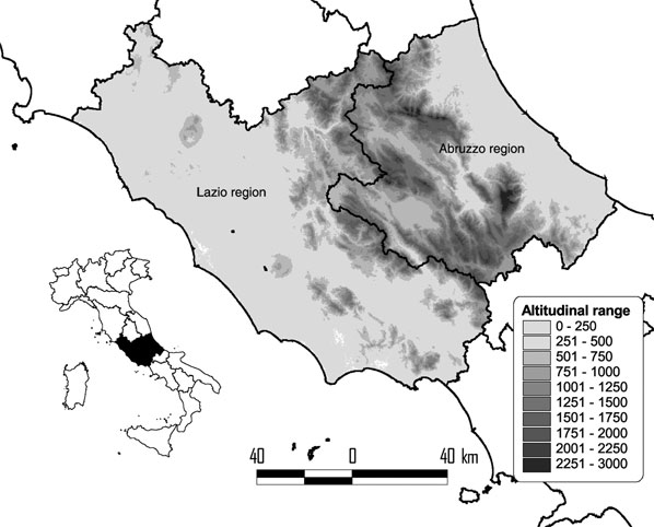
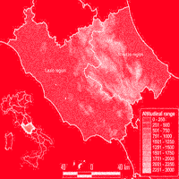
The study area consists of two Italian regions (Lazio and Abruzzo) located in Central Italy between the Tyrrhenian and Adriatic coasts and covers about 28000 km2 (Fig. 1). The area is characterised by strong climatic, topographical and geological variability. The coastal areas are characterised by a Mediterranean climate, while the inner part has a temperate climate, with an Alpine-type climate only in the highest peaks (Gran Sasso mountain, 2912 m a.s.l.).
Forests, following the FAO forest definition ([9]), currently occupy an area of about 6720 km2. Since the end of the Second World War, the forested areas have increased because of the abandonment of traditional silvicultural activities, especially in the Apennine mountains ([10]). Evergreen forests of Quercus ilex and Q. suber (the latter only along the western Tyrrhenian side) potentially occupy the low-land areas along the coasts, while the inner hills are characterised by deciduous forest (Q. cerris and Q. pubescens). The sub-mountain and mountain belts are respectively dominated by Ostrya carpinifolia and Fagus sylvatica woods.
Data set
The data source for this study was the IN.DE.FO. of Italy for the study area ([1]). It comprises 912 plots collected on the vertices of a 3x3 km grid. The data were summarised for individual forest plots to calculate an Importance Value (IV) as a measure of abundance for each species according to the following formula:
where x is one of the considered species, NS is the number of stems of a plot and BA is the basal area of the plot calculated using the diameter at breast height of each one of the stems. In monotypic stands, the IV could reach a maximum of 200.
We analysed sixteen species that are the most abundant in the study area: Acer campestre, Acer obtusatum, Acer pseudoplatanus, Carpinus betulus, Carpinus orientalis, Castanea sativa, Fagus sylvatica, Fraxinus ornus, Quercus cerris, Quercus frainetto, Quercus ilex, Quercus pubescens, Quercus robur, Quercus suber, Ostrya carpinifolia, Ulmus minor. The species listed above belong either to Mediterranean (M - 2 species), Sub-Mediterranean (SM - 8 species) or Eurosiberian (E - 6 species) chorological types (see Tab. 2 - [31]). In order to explain the response of the species to climate change, Ellenberg’s indicator values ([8]), revised for Italy by Pignatti ([32]), for temperature and moisture were used. These indicator values describe the ecological optima for the species along ecological gradients using an ordinal scale, i.e., temperature: 1 (cold, alpine environment) to 12 (hot, subdesertic environment); moisture: 1 (dry environment, arid soil) to 12 (water environment).
Tab. 2 - Validation of the regression tree model. N is the number of sample plots. R is the correlation between measured and predicted IV. OA_Ve and OA_Va are the omission accuracy for the whole data set (verification) and for the 30 % of the validation data set respectively. Abbreviations for chorology: M, Mediterranean; SM, Sub-Mediterranean; E, Eurosiberian.
| Species | Chorology type | N | R | OA_Ve | OA_Va |
|---|---|---|---|---|---|
| Quercus ilex | M | 102 | 0.77 | 0.79 | 0.68 |
| Quercus suber | M | 43 | 0.63 | 0.77 | 0.67 |
| Mean | - | - | 0.70 | 0.78 | 0.68 |
| Acer campestre | SM | 106 | 0.72 | 0.67 | 0.65 |
| Acer obtusatum | SM | 85 | 0.63 | 0.85 | 0.74 |
| Carpinus orientalis | SM | 54 | 0.53 | 0.63 | 0.61 |
| Castanea sativa | SM | 85 | 0.78 | 0.89 | 0.85 |
| Fraxinus ornus | SM | 141 | 0.63 | 0.76 | 0.68 |
| Ostrya carpinifolia | SM | 177 | 0.74 | 0.81 | 0.75 |
| Quercus cerris | SM | 287 | 0.81 | 0.97 | 0.92 |
| Quercus frainetto | SM | 41 | 0.60 | 0.82 | 0.71 |
| Quercus pubescens | SM | 361 | 0.80 | 0.98 | 0.86 |
| Mean | - | - | 0.69 | 0.82 | 0.75 |
| Acer psedoplatanus | E | 88 | 0.68 | 0.84 | 0.75 |
| Carpinus betulus | E | 73 | 0.62 | 0.60 | 0.64 |
| Fagus sylvatica | E | 263 | 0.90 | 0.99 | 0.95 |
| Quercus robur | E | 59 | 0.57 | 0.79 | 0.69 |
| Ulmus minor | E | 50 | 0.76 | 0.70 | 0.72 |
| Mean | - | - | 0.71 | 0.78 | 0.75 |
Environmental variables
Very high resolution (30 arc-seconds) current climatic surfaces were obtained by interpolating climatic data (average of the 1961-1991 period) from 210 stations for precipitation and 151 for temperature through universal kriging (i.e., simple kriging with trend function defined on the basis of a set of co-variates) that has been proven to produce reliable estimates at a regional scale ([4]). Future projections for 2080 (midpoint of the period 2070-2099) were derived using one general circulation model experiment (HadCM3 - [24]). The GCM projected the mean climate under one rather extreme scenario: the Intergovernmental Panel on Climate Change Special Report on Emissions Scenarios (IPCC SRES) A1FI storyline ([25]). Current and projected climatic data were obtained from HadCM3 runs. The difference between the current and future climate was calculated. The difference was statistically downscaled to a 30 arc second using the “thin plane spline” spatial interpolation ([23]). The values were then applied to the measurements of the current climate to produce very high resolution climatic scenario.
Climatic data which influence plant survival and growth were chosen: mean annual temperature, mean minimum temperature of the coldest month, mean maximum temperature of the hottest month, annual, summer and winter precipitations. Moreover, a moisture index was used based on the following formula:
where P is the mean annual precipitation, and ETp is the potential evapotranspiration; ETp has been calculated using the Jensen-Haise equation ([18]):
where RS is the annual potential solar radiation (KiloJoule) and T is the mean annual temperature.
The annual potential solar radiation was calculated using a specific module implemented in the Grass software GIS ([14]). This model takes into account solar constant, Earth-Sun distance, solar geometry and incident angles at each location (slope aspect), cast-shadowed and self-shadowed areas, and direct versus diffuse radiation.
A slope map and a simplified geological map (scale 1:100.000, Servizio Geologico d’Italia, APAT) were also used. The geological map was a surrogate for pedological information. ArcGIS 9.0 was used to collect, store and manipulate IV as well as environmental data in raster format. The complete list of environmental variables is shown in Tab. 1.
Tab. 1 - List of the selected environmental variables.
| Environmental variable | Acronym |
|---|---|
| Mean Annual Temperature | MAT |
| Mean Maximum Temperature of the Hottest Month | MTH |
| Mean Minimum Temperature of the Coldest Month | MTC |
| Annual Precipitation | AP |
| Summer Precipitation | SP |
| Winter Precipitation | WP |
| Moisture Index | Mi |
| Slope | Slo |
| Geology: - Alluvial sediments - Arenaceous rocks - Carbonated rocks - Clayey formations - Sands - Volcanic rocks |
- |
Statistical analysis
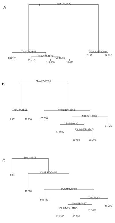
A Regression Tree (RT) and a Stepwise Multiple Linear Regression (MLR) models were compared in order to quantify the relationship between environmental factors and the species abundance. The theory of MLR is quite well known and will not be reported here (interested readers should refer to [26]). RT models have been widely used in the last few years to study the potential distribution of tree species abundance in the eastern United States ([15], [16], [17]). They are based on a recursive data partitioning algorithm that splits the data into subsets based on a single, best predictor variable. The algorithm proceeds by splitting these subsets using the remaining covariate values. The output is a tree with branches and terminal nodes (Fig. 3). The predicted value at each terminal node is the average at that node, which can be considered as relatively homogeneous. Thus, the substantial difference between regression trees and linear regression models is in the effects of the adopted covariates set. In the latter case, the effect is linear and constant over the whole range of covariate values. In the former, the effect of the covariates is neither linear nor constant, producing a categorization of the (quantitative) covariate best predicting the observed response. Moreover, the obtained hierarchical structure gives a simple and effective way to understand the covariates’ impact on the observed response; the corresponding role in terms of response prediction can be based on the ordering produced by the increase in the percentage of response variability which is accounted for by each split. The interested reader should refer to Breiman et al. ([7]). We estimated both models using S-PLUS ([39]) considering the species IV as the response variable and the environmental covariates listed in Tab. 1. The RTA model was generated after pruning the full tree.
Fig. 3 - Tree diagrams for A - Fagus sylvatica, B - Quercus cerris, C - Quercus ilex. The abundance of each variable is proportional to the length of the corresponding couple of branches. The numbers at the termination of each node of the tree show the average IV at that node.
We randomly put aside 30% of the data (test set), and trained the models on the remaining 70% (training set). The RTA and the MLR were evaluated on the test set using the mean RMSE between the current and predicted IVs for each species. The best model was evaluated by calculating both the correlation between current and predicted IV as well as the so-called Omission Accuracy (OA) measure. To calculate this last measure, we categorized the observed and predicted IVs into binary variable indicating if the values were over a certain threshold. The threshold was set at 2 IV since the values below were characterised by a high uncertainty. For each species, the OA formula is (SP/(SP+SO)*100), where SP is the number of areas with observed values over the threshold where the species was correctly predicted as present and SO is the number of areas with observed values over the threshold where the species was incorrectly predicted as absent. Because of the sampling approach we used, classification accuracy was not calculated for the test set; indeed, the absence of a species at a given sampling plot does not imply its absence over the 3 x 3 km grid.
The results obtained through the final model were used to produce maps of both current and future potential distribution under a scenario of changed climate assuming unlimited dispersal capacity of the species. The predicted potential distribution was obtained by replacing the climate variables with those obtained from the HadCM3 GCM; predicted values were then imported into ArcGIS to produce the corresponding maps.
The effects of climate change on species distribution were evaluated by calculating the percentage changes in the potential area as well as on the mean IV and altitude.
Results
Comparison and evaluation of models
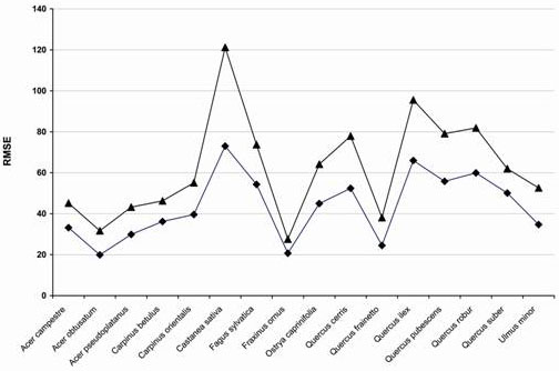
The comparison between RMSE values corresponding to both models for all of the analysed species shows that RTA always outperformed MLR, in terms of predicting species distribution for the training set (Fig. 2). For this reason, RTA was chosen as the best method; the corresponding performance measures are reported in Tab. 2. The number of plots for each species used for the modelling process is a measure of the abundance of the species within the study area. Quercus pubescens and Quercus cerris were the most widespread species, respectively with 361 and 287 plots. These were followed by Fagus sylvatica (263 plots). In contrast, Quercus frainetto and Quercus suber, the rarest species, were limited to the coastal areas characterised by acidic soils ([3]). The correlation between observed and predicted IV values ranged between 0.53 of Carpinus orientalis to 0.90 of Fagus sylvatica. Predicted current distributions match well the inventory data for almost all the species, with Fagus sylvatica, Quercus pubescens and Quercus cerris showing the highest omission accuracy values in both the verification and the validation data set. Only three species, Carpinus orientalis, Carpinus betulus and Acer campestre had values of omission accuracy index below 70%.
Fig. 2 - Comparison between the RMSE value of the regression tree analysis (black diamonds) and that of the multiple linear regression (black triangles) for all the species.
Environmental correlates of tree species abundance
The tree diagrams produced by RTA analysis are shown in Fig. 3a for a Eurosiberian species (Fagus sylvatica), in Fig. 3b for a Sub-Mediterranean species (Quercus cerris) and in Fig. 3c for a Mediterranean one (Quercus ilex). As aforementioned, the tree diagrams proved to be a useful way to highlight the interactions between environmental variables and species distribution ([15], [47], [46]). The length of tree diagram branches is proportional to the variance explained by the current split. The terminal nodes of the data set indicate the average IV value for the relatively homogeneous subset. Fagus sylvatica is mainly found in areas with an average temperature of less than 24 °C for the hottest month. In areas above this climatic limit, the species can only be found in very small areas characterised by a high amount of summer precipitation (above 200 mm). In fact, in those areas, it is still possible to find remnant patches of Fagus sylvatica, residual of previous cycles of expansion of the species ([20]). The maximum temperature of the hottest month is also the most important variable for Quercus cerris, one of the most widespread species in the area. In this case the species has a threshold of 27.8 °C, above which it can be found only in areas characterised by high winter precipitation (> 260 mm), excluding the hyper humid areas (moisture index values > 1). In contrast, the average minimum temperature the most important variable in influencing the spatial distribution of Quercus ilex. In fact, the species is absent in areas characterised by very low winter temperature (MTC < 2 °C). The other important variables are: the presence of a geological substratum of carbonated rocks and summer aridity, since the species is well adapted to these conditions.
Potential current and future distribution of tree species abundance
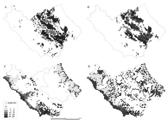
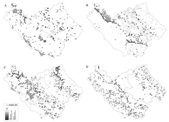
According to the estimated model, Quercus pubescens and Quercus cerris are the species with the widest potential distribution (Tab. 3). Fagus sylvatica and Castanea sativa have a smaller potential area, but they also have a high average IV, 83.5 and 60.9 respectively. This means that these two species tend to form almost mono-specific forests. Instead, Quercus frainetto and Acer pseudoplatanus have the smallest potentiality in terms both of area and IV. Generally they are associated, respectively, with Quercus cerris and Fagus sylvatica. Once we had established a reasonably reliable (in terms of RMSE) model for all the species, current climatic data were replaced with those obtained through HadCM3 GCM in order to evaluate potential future distribution. The prediction of potential species distribution shows significant changes for many species: there is a general trend towards an increasing mean altitude, with the exception of Fraxinus ornus. Five species should increase both their area and IV (Group 1, Tab. 2), while six species should reduce both these parameters. Moreover, Acer campestre and Carpinus betulus present an increasing area and a decreasing IV, while Carpinus orientalis, Fraxinus ornus and Quercus frainetto show an opposite trend. As an example, the maps of the current potential and future potential distribution of four species belonging to the four different groups identified in relation to their response to changes in the climatic scenario are shown in Fig. 4 and Fig. 5. The two well-modelled species (Fagus sylvatica and Quercus ilex) show a good correspondence between the distribution of sample plots and the predictions (Fig. 4), while the two fairly-modelled species (Fraxinus ornus and Carpinus betulus) show a higher number of incorrectly predicted “absent” plots (Fig. 5). The application of the climate scenario determines a noticeable reduction of area and IV of Fagus sylvatica (respectively - 29% and -3%), the expansion of Quercus ilex (Area +74.6%, IV +2.4%), the transformation of Carpinus betulus from the status of sporadic, localised extra-zonal species to that of a more widespread species in the submountain areas as shown by the increase of area (+81.5 %) and average altitude (+94.9), and the strong reduction in area of Fraxinus ornus area (-20%) and a contemporaneous increase of its IV (+2.2 - Tab. 3).
Tab. 3 - Current, future and percentage of change of the potential area (km2) and average IV and altitude (m); the percentage changes are due to the HadCM3 model outputs; Ellenberg’s scores for temperature (T) and moisture (M). In the last columns, X means the species has a wide spectrum for that parameter. Abbreviations for chorology: M, Mediterranean; SM, Sub-Mediterranean; E, Eurosiberian.
| Group | Species | Chorology type |
Area (km2) | IV | Altitude (m) | T | M | ||||||
|---|---|---|---|---|---|---|---|---|---|---|---|---|---|
| Current | Future | % | Current | Future | % | Current | Future | % | |||||
| Group 1: +IV +Area |
Quercus cerris | SM | 24417 | 24832 | 1.7 | 46 | 67.3 | 46.3 | 408.3 | 576.1 | 41.1 | 8 | 4 |
| Quercus ilex | M | 9423 | 16453 | 74.6 | 37 | 37.9 | 2.4 | 212.4 | 342 | 61 | 9 | 3 | |
| Quercus pubescens | SM | 24732 | 27947 | 13 | 60.7 | 81.7 | 34.6 | 414.3 | 541.5 | 30.7 | 8 | 3 | |
| Quercus suber | M | 3006 | 5282 | 75.7 | 40.7 | 48.1 | 18.2 | 75.2 | 79.3 | 5.5 | 8 | 3 | |
| Ulmus minor | E | 2682 | 2926 | 9.1 | 24.9 | 33.4 | 34.1 | 163.2 | 216.6 | 32.7 | 7 | X | |
| Group 2: -IV -Area |
Acer obtusatum | SM | 3393 | 1863 | -45.1 | 13.4 | 11.6 | -13.4 | 698.6 | 1159 | 65.9 | 5 | 6 |
| Acer pseudoplatanus | E | 2115 | 584 | -72.4 | 12.7 | 10.6 | -16.5 | 972.7 | 1297.6 | 33.4 | 5 | 6 | |
| Castanea sativa | SM | 5175 | 5051 | -2.4 | 60.9 | 38.4 | -36.9 | 578.2 | 932.6 | 61.3 | 8 | X | |
| Fagus sylvatica | E | 8946 | 6352 | -29 | 83.5 | 81 | -3 | 1144.2 | 1330.7 | 16.3 | 5 | 5 | |
| Ostrya caprinifolia | SM | 7497 | 4183 | -44.2 | 24.8 | 23 | -7.3 | 736.5 | 1082.7 | 47 | 8 | 4 | |
| Quercus robur | E | 5634 | 3747 | -33.5 | 28.9 | 21.7 | -24.9 | 238.2 | 248.2 | 4.2 | 6 | 6 | |
| Group 3: -IV +Area |
Acer campestre | SM | 6255 | 7400 | 18.3 | 25.3 | 18.5 | -26.9 | 330.5 | 358.3 | 8.4 | 7 | 5 |
| Carpinus betulus | E | 3645 | 6616 | 81.5 | 14.7 | 8.1 | -44.9 | 442.7 | 862.8 | 94.9 | 6 | X | |
| Group 4: +IV -Area |
Carpinus orientalis | SM | 1242 | 532 | -57.2 | 18.2 | 30.9 | 69.8 | 616.8 | 1244.1 | 101.7 | 7 | 3 |
| Fraxinus ornus | SM | 7101 | 5681 | -20 | 13.4 | 13.7 | 2.2 | 468.6 | 380 | -18.9 | 8 | 3 | |
| Quercus frainetto | SM | 3645 | 2278 | -37.5 | 12.8 | 21.7 | 69.5 | 63.7 | 79.8 | 25.3 | 6 | 6 | |
Fig. 4 - Current and future predicted potential distribution of Fagus sylvatica (A, B) and Quercus ilex (C, D).
Fig. 5 - Current and future predicted potential distribution of Carpinus betulus (A, B) and Fraxinus ornus (C, D).
Discussion
Model comparison
RTA had a better performance in modelling the spatial distribution of all the analysed species compared to MLR (Fig. 2). This result can be explained since RTA neither relies on linearity of covariate effects nor on constant effects throughout the analysed area. This could mean that RTA could readily accommodate departures from a homogeneous model, accounting for local discontinuities as well as for local dependencies. These differences in model features are substantial if the observed species distribution is highly scattered and potentially heteroscedastic, with local hotspots and wide areas with non-relevant IV values.
Actual and potential current distribution of tree species abundance
Using results from RTA, a significant correlation between number of sample plots where the species was recorded and model accuracy was found (Tab. 2). Indeed, species whose distribution is more strongly linked to local climatic conditions (Quercus pubescens, Quercus cerris and Fagus sylvatica) show a higher accuracy in model predictions. Instead, rare species (mainly extrazonal), being at the edge of their distribution or having more specific habitat requirements, were less accurately modelled (e.g., Carpinus orientalis and Carpinus betulus).
The main chorological component was represented by Sub-Mediterranean deciduous species (8 species), showing on average the best accuracy values (Tab. 2). The second group was formed by Eurosiberian species (6), while only two Mediterranean evergreen sclerophyllous species have a spatial distribution wide enough to be included in this analysis: Quercus ilex and Quercus suber. Species belonging to the same chorological type and thus sharing the same geographical distribution have different capacities of adaptation to local conditions. For this reason a Eurosiberian species such as Fagus sylvatica has, in the study area, a wide distribution well modelled by this climatic model, while Carpinus betulus, also Eurosiberian, is more localized, dependent on factors other than the climatic ones and fairly modelled.
The deciduous tree species are more abundant than the sclerophyllous evergreen ones in terms of species number and spatial distribution. This result depends on the fact that the study area, despite its Mediterranean location, is characterized mainly by a temperate climate because of the effects of the Apennine mountains, which intercept the humid winds from the sea, thus causing a rainfall increase ([4]). Moreover, in this area, the dominance of deciduous species has characterised almost all of the inter-glacial periods during the last 250000 years ([11]). As shown by the analysis of lake sediments, during the Holocene a progressive increase of pollen of sclerophyllous tree species, mainly Quercus ilex, did occur starting from 1.500 B.C. This change can neither be explained by climate change nor by the use of fire to clear land for agriculture ([19]). For this reason, it may be hypothesized the occurrence of the same process recorded in southern France ([34]): the prolonged exploitation of forests caused increasing soil erosion, especially in the southern exposures of the Apennine mountains, favouring Quercus ilex, which is more adapted to xeric environments than deciduous species such as Quercus pubescens and Quercus cerris. This hypothesis may also explain the current presence of areas with potentially high IV in the inner part of the Lazio region (see Fig. 4c).
Other examples of tree species expansion due to human intervention are those of Castanea sativa for timber and food production dating back to the Greco-Roman age and the more recent example of Quercus suber in the western side of the Italian peninsula for the production of cork ([36]). Those examples are, however, the exception in a general framework, where a general reduction of the distribution of tree species has occurred after the post-glacial recolonisation as a result of deforestation and land use changes ([33]). This process was not continuous and ceaseless, depending on the historical socio-economic conditions: as an example, the secondary recolonization of the mountain Apennine pastures by Fagus sylvatica occurred during the last decades due to the reduction of traditional breeding activities ([3]).
Future potential distribution
A general increase of the average potential altitude is predicted applying the HADCM3 climate scenario for year 2080. However if area and abundance are analysed, four different trends can be identified: species that could be advantaged by the predicted climate change (Tab. 3, group 1), species that could suffer a strong reduction of area and abundance (Group 2) and species showing contrasting behaviour in relation to area and abundance (Group 3, 4).
According to the chorological types, the two Mediterranean species (Quercus ilex and Quercus suber) are likely to be favoured by the predicted increased drought, while the species belonging to the two other chorological types show quite differentiated behaviour. According to the Ellenberg’s scores, the more thermophilous and xerophilous species should be favoured by the predicted drought (Group 1, Tab. 3). In contrast, mesophilous species should suffer a strong reduction of area and abundance (Group 2). For the two remaining groups, there is not a clear ecological explanation for their particular trends. However, it should be noticed that they are formed by fairly modelled species, such as Carpinus orientalis, Carpinus betulus and Quercus frainetto. Indeed, the above species are at the edge of their natural range, so it may be hypothesized that their presence in the study area is linked to other variables (e.g., edaphic factors) not included in the model. On the other hand, Acer campestre and Fraxinus ornus are low-frequency species spread over different plant communities, so a better definition of their climatic niche is expected to be obtained by enlarging the study area.
Conclusions
RTA has proven to be efficient for the identification of the environmental variables driving the current distribution and abundance of tree species at a regional scale. Only Mediterranean species are likely to be favoured by the predicted climate change, while for the two other chorological types (Sub-Mediterranean and Eurosiberian) the response seems to be species-specific depending on the autoecological characteristic of each species. A more complete picture of the potential effects of climate change would be obtained by analysing the whole Italian peninsula considered as a biogeographical unit and including a detailed land use map as a measure of fragmentation and anthropization of the territory, influencing the expected shift of species.
Acknowledgements
This work has been carried out in the framework of CONECOFOR (CONtrollo ECOsistemi FORestali), the intensive monitoring programme of forest ecosystems in Italy. The programme is framed within the Pan-European Level II Monitoring of Forest Ecosystems. It is co-sponsored by the European Union under the Regulation no. 2152/2003 “Forest Focus” and co-operate with the UN/ECE ICP-Forests and the UN/ECE ICP-Integrated Monitoring of Ecosystems. CONECOFOR is managed by Corpo Forestale dello Stato, Divisione 6a, CONECOFOR Board, acting also as National Focal Center (NFC) of Italy within the EU and UN/ECE programmes.
References
Gscholar
Gscholar
Gscholar
Gscholar
Gscholar
Gscholar
Gscholar
Gscholar
Gscholar
Gscholar
Gscholar
Gscholar
CrossRef | Gscholar
Authors’ Info
Authors’ Affiliation
F Francesconi
L Scarnati
M De Sanctis
F Bruno
Department of Plant Biology, “La Sapienza” University of Rome, p.le A. Moro 5, I-00185 Rome (Italy)
Department of Statistics, “La Sapienza” University of Rome, p.le A. Moro 5, I-00185 Rome (Italy)
Corresponding author
Paper Info
Citation
Attorre F, Francesconi F, Scarnati L, De Sanctis M, Alfò M, Bruno F (2008). Predicting the effect of climate change on tree species abundance and distribution at a regional scale. iForest 1: 132-139. - doi: 10.3832/ifor0467-0010132
Academic Editor
Gabriele Bucci
Paper history
Received: Jul 18, 2007
Accepted: Aug 13, 2008
First online: Aug 27, 2008
Publication Date: Aug 27, 2008
Publication Time: 0.47 months
Copyright Information
© SISEF - The Italian Society of Silviculture and Forest Ecology 2008
Open Access
This article is distributed under the terms of the Creative Commons Attribution-Non Commercial 4.0 International (https://creativecommons.org/licenses/by-nc/4.0/), which permits unrestricted use, distribution, and reproduction in any medium, provided you give appropriate credit to the original author(s) and the source, provide a link to the Creative Commons license, and indicate if changes were made.
Web Metrics
Breakdown by View Type
Article Usage
Total Article Views: 68788
(from publication date up to now)
Breakdown by View Type
HTML Page Views: 57283
Abstract Page Views: 5335
PDF Downloads: 4951
Citation/Reference Downloads: 77
XML Downloads: 1142
Web Metrics
Days since publication: 6455
Overall contacts: 68788
Avg. contacts per week: 74.60
Article Citations
Article citations are based on data periodically collected from the Clarivate Web of Science web site
(last update: Mar 2025)
Total number of cites (since 2008): 16
Average cites per year: 0.89
Publication Metrics
by Dimensions ©
Articles citing this article
List of the papers citing this article based on CrossRef Cited-by.
Related Contents
iForest Similar Articles
Research Articles
Potential impacts of regional climate change on site productivity of Larix olgensis plantations in northeast China
vol. 8, pp. 642-651 (online: 02 March 2015)
Review Papers
Impacts of climate change on the establishment, distribution, growth and mortality of Swiss stone pine (Pinus cembra L.)
vol. 3, pp. 82-85 (online: 15 July 2010)
Research Articles
Predicting impacts of climate change on forest tree species of Bangladesh: evidence from threatened Dysoxylum binectariferum (Roxb.) Hook.f. ex Bedd. (Meliaceae)
vol. 10, pp. 154-160 (online: 25 May 2016)
Review Papers
Climate change impacts on spatial distribution, tree-ring growth, and water use of stone pine (Pinus pinea L.) forests in the Mediterranean region and silvicultural practices to limit those impacts
vol. 14, pp. 104-112 (online: 01 March 2021)
Research Articles
Model-based assessment of ecological adaptations of three forest tree species growing in Italy and impact on carbon and water balance at national scale under current and future climate scenarios
vol. 5, pp. 235-246 (online: 24 October 2012)
Research Articles
Is Pinus pinea growth affected by climate change in western Anatolia?
vol. 18, pp. 93-101 (online: 28 April 2025)
Research Articles
Impact of climate change on tree-ring growth of Scots pine, common beech and pedunculate oak in northeastern Germany
vol. 9, pp. 1-11 (online: 13 October 2015)
Research Articles
Hearing nature’s heartbeat: towards large-scale real-time forest monitoring network in Italy
vol. 18, pp. 202-211 (online: 09 August 2025)
Research Articles
Reviewing climatic traits for the main forest tree species in Italy
vol. 12, pp. 173-180 (online: 15 March 2019)
Research Articles
An assessment of climate change impacts on the tropical forests of Central America using the Holdridge Life Zone (HLZ) land classification system
vol. 6, pp. 183-189 (online: 08 May 2013)
iForest Database Search
Search By Author
Search By Keyword
Google Scholar Search
Citing Articles
Search By Author
Search By Keywords
PubMed Search
Search By Author
Search By Keyword

