Yield of forests in Ankara Regional Directory of Forestry in Turkey: comparison of regression and artificial neural network models based on statistical and biological behaviors
iForest - Biogeosciences and Forestry, Volume 16, Issue 1, Pages 30-37 (2023)
doi: https://doi.org/10.3832/ifor4116-015
Published: Jan 22, 2023 - Copyright © 2023 SISEF
Research Articles
Abstract
Models of forest growth and yield provide important information on stand and tree developments and the interactions of these developments with silvicultural treatments. These models have been developed based on assumptions such as independence of observations, uncorrelated error terms, and error terms with constant variance; if these factors are absent, there may be problems with multicollinearity, autocorrelation, or heteroscedasticity, respectively. These problems, which have several adverse effects on parameter estimates, are statistical phenomena and must be avoided. In recent years, the artificial neural network (ANN) model, thanks to its superior features such as the ability to make successful predictions and the absence of the requirement for statistical assumptions, has been commonly used in forestry modeling. However, while goodness-of-fit measures were taken into consideration in the assessment of ANN models, the control of the biological characteristics of model predictions was ignored. In this study, variable-density yield models were developed using nonlinear regression and ANN techniques. These modeling techniques were compared based on some goodness-of-fit measures and the principles of forest yield. The results showed that ANN models were more successful in meeting expected biological patterns than regression models.
Keywords
Introduction
Regression models have been widely used to maximize the explained variation in forest measurements, such as individual tree heights, individual tree diameter increments, stand basal areas, stand volumes, and site indexes ([43]). The reliability of regression models depends on the fulfillment of certain statistical assumptions ([49]). Because forest inventory data are spatially or temporally correlated ([17]), the statistical assumptions are usually violated, and this leads to biased estimates ([47]). To deal with the statistical problems, the autoregressive modeling technique ([22]) and mixed-effect modeling technique ([26]) can be used. However, some issues associated with these modeling techniques have remained in question ([45]). For instance, it may be problematic to determine the parameter of random effects in a mixed effects model. While some studies take goodness-of-fit measures into consideration ([33], [38]), others consider the variance in the estimated parameters ([12], [8]).
Artificial neural network (ANN) models that are independent of statistical assumptions have been widely used in forestry modeling. In earlier studies, ANN models were commonly employed to classify forest characteristics ([25], [14]), but recently they have been used for both the classification and prediction of forest characteristics such as site index ([27]) and stand basal area ([7]).
Most researchers have paid attention to goodness-of-fit statistics in evaluating the performance of ANN models ([3], [26]). However, growth and yield predictions for forests should also be evaluated based on the principles of forest growth and yield ([46], [39]). To our knowledge, no studies have explored the success of ANN models in meeting biological expectations. In addition, many researchers have provided very little information about the setting of the network parameters. This study found that when the network parameters are not correctly set, the predictions may be implausible from a biological point of view even if the statistical scores are satisfactory.
The objectives of this study were to (i) develop variable-density yield models using a modified Gompertz model and an ANN model and (ii) compare their performances based on goodness-of-fit statistics and the principles of forest yield.
Materials and methods
Study area
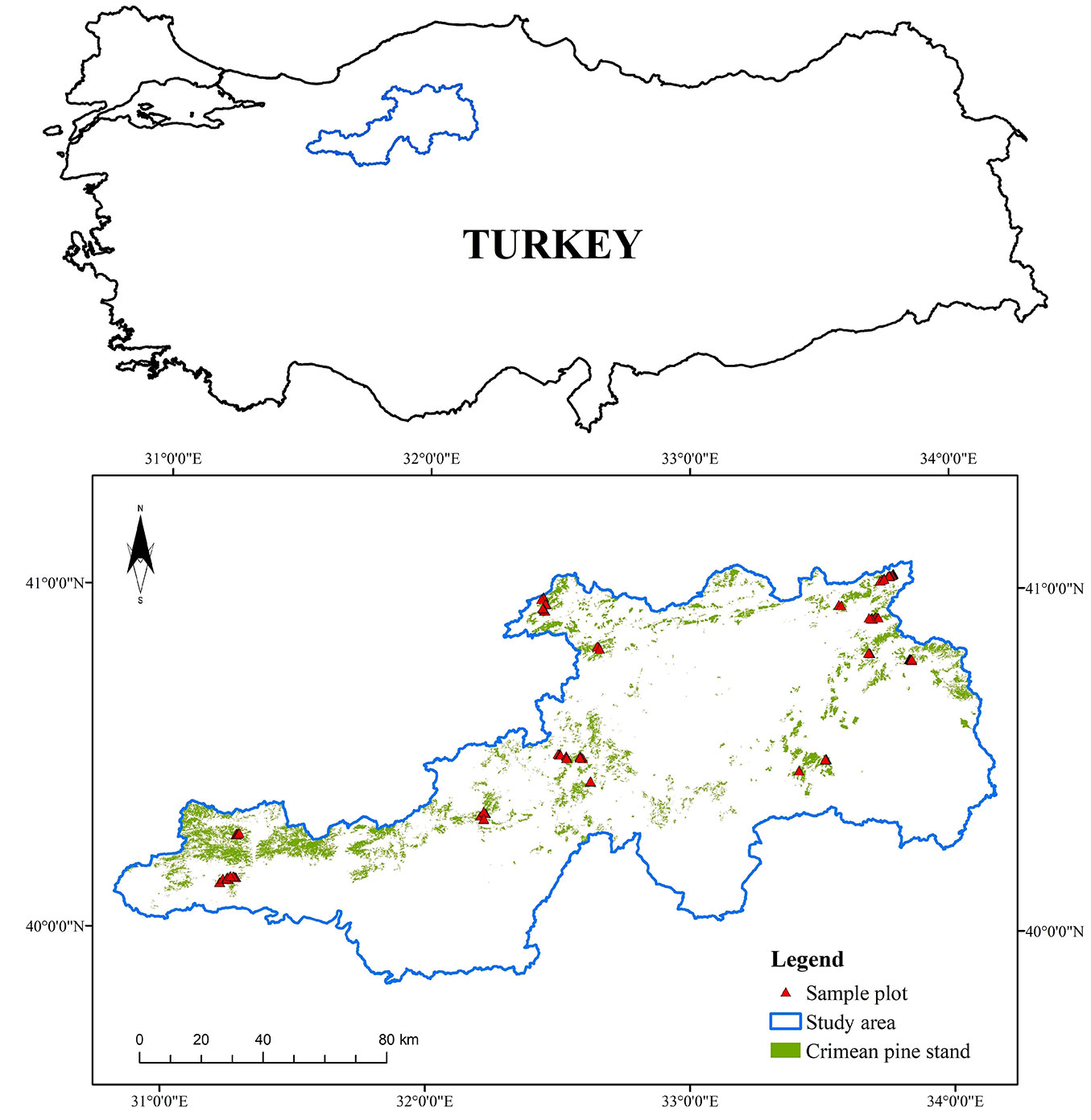
In this study, natural monospecific Crimean pine stands (Pinus nigra Arnold. subsp. pallasiana Lamb.) were sampled. They cover 44.8% (136,985.96 ha) of the total forest area in the Ankara Regional Directory of Forestry in Turkey ([18]). Other common species in this area are various oak species (Quercus cerris L., Quercus infectoria Olivier, Quercus frainetto Ten., Quercus robur L., and Quercus petraea Matt.) and the Scots pine (Pinus sylvestris L.). Fig. 1 shows the sample plots and location of the study area (33° 48′ 54″ - 37° 10′ 06″ N; 39° 51′ 28″ - 41° 02′ 47″ E). The elevation of the study area varied between 239 m and 2541 m above mean sea level. The mean annual precipitation and mean annual temperature were 393.2 mm and 11.9 °C, respectively ([42]).
Field measurements
Forest yield models should ideally be developed using data from permanent sample plots. However, this study used data from temporary sample plots because there were no permanent sample plots of natural monospecific Crimean pine stands grown in the study area. The sample plots inventoried were selected to be representative of the range of site indexes, stand densities, and stand ages. A total of 180 sample plots were randomly chosen; in each, a circular sampling scheme was adopted because the stands, which have different stand densities in same site index and have different ages in same site index and stand density, should be adequately sampled. If the number of samples is insufficient in terms of site index, stand density, and age, a variable-stand density model may not meet the principles of forest yield. The area of the sample plots was 400, 600, or 800 m2 according to the crown closure of the plots. This study followed the forest management guidelines of Turkey in determining the area of the sample plots ([2]). The measurements in the sample plots were: (i) all trees (≥ 4 cm in diameter at breast height) were measured at 1.3 m above the ground; (ii) the mean dominant height of the sample plots was calculated by averaging the height of a certain number of trees corresponding to the 100 tallest trees per hectare; then, the site index value of the sample plots was assigned using the site index table developed by Kalipsiz ([24]); (iii) the mean age of the sample plots was calculated by averaging the age of the representative four trees considering the quadratic mean diameter of the sample plots; (iv) to establish height-diameter relationships, the height of 10 trees having different diameters at breast height in each sample plot was subsampled.
Tab. 1 shows the descriptive statistics of the Crimean pine stands.
Tab. 1 - Descriptive statistics of Crimean pine stands studied in this study. (Dq): quadratic mean diameter; (Hq): quadratic mean height; (A): age; (G): basal area; (N): stem number; (V): volume derived from the double entry tree volume equation V = 0.000202 · d1.602553 h0.969154 ([4]); (SI): site index; (SD): stand density ([9]).
| Variables | n | Min | Max | Mean | STD |
|---|---|---|---|---|---|
| Dq (cm) | 180 | 2.00 | 56.30 | 27.14 | 10.89 |
| Hq (m) | 180 | 2.00 | 31.30 | 15.25 | 6.31 |
| A (year) | 180 | 13.50 | 161.67 | 74.11 | 32.87 |
| G (m2 ha-1) | 180 | 2.00 | 70.00 | 31.11 | 14.46 |
| N (number ha-1) | 180 | 137.50 | 1550.00 | 630.02 | 327.59 |
| V (m3 ha-1) | 180 | 7.00 | 921.67 | 323.79 | 216.15 |
| SI (m) | 180 | 10.00 | 34.00 | 21.16 | 6.68 |
| SD | 180 | 1.25 | 16.92 | 6.24 | 2.70 |
Regression-type variable-density yield models
The selection of a suitable yield function is essential for modeling forest development. In forestry modeling, sigmoid functions such as the Lundqvist-Korf, Richards, and Hossfeld IV/McDill-Amateis functions have been widely used ([5]) owing to their flexible forms. They produce the most appropriate curves for any stand characteristic depending on the site index and stand density. In this study, the nonlinear variable-density yield models (eqn. 1 to eqn. 6) were developed using the Gompertz function, which is one of the Richards-type growth functions. To facilitate the selection of starting values for the parameters, a solver tool was developed using the Generalized Simulated Annealing package in the R environment (see Appendix 1 in Supplementary material).
where G is the stand basal area (m2 ha-1), V is the stand volume (m3 ha-1), N is the number of trees (ha), A is the stand age (years), SD is the stand density developed by Curtis ([9]), SI is the site index (m), and b1, …, b3, and a1, …, a4 are the regression coefficients to be estimated.
In general, the variable-density yield models include SI, SD, and A as explanatory variables. In addition, the different explanatory variables derived from SI, SD, and A (e.g., ln(SI), ln(SD), SI2) can be used to effectively describe the development of the stands. In this study, the prediction accuracy and the principles of forest yield were considered when deciding which variable to use. The principles of forest yield considered in this study are: (i) V and G increase with increasing SI, but N declines; (ii) V, G, and N increase with increasing SD; (iii) V and G increase with age; (iv) N decreases with age - this reduction is generally high in young stands due to strong inter-tree competition, which leads to a high probability of mortality ([32]); (v) V, B, and N may develop in totally different ways depending on the SI and SD in the managed forests - the stands of the same age but in different SIs and SDs may have a variable proportion of yield; therefore, the S-shape of the yield curves should be characterized by the polymorphic curves; (vi) the yield curves should reach an asymptote ([19]) - in the absence of an asymptote, the long-term forecasts of the stand variables are limited and may even be invalid.
Artificial neural network type variable-density yield models
It is crucial to construct an ANN model that is consistent with the principles of forest yield. If ANN’s parameters are not properly managed, the produced ANN model will lead, in general, to unreasonable results ([21]). Therefore, this study developed a promising modeling framework to meet the principles of forest yield.
An ANN model includes three fully connected layers: the input layer, hidden layer, and output layer. Each input with an appropriate weight is taken into the input layer without any data processing. The weighted inputs with added bias values are passed to the hidden layer through an activation function. Then, the resulting data are propagated forward to the next layer. This process is continued until the final output has been produced.
The various types of activation functions are selected according to the type of problem. The sigmoid (i.e., logistic and hyperbolic tangent functions) and linear activation functions seem to be suitable for biological relationships in the hidden layer and output layer, respectively ([35], [3]). The activation functions may significantly influence the performance of ANN models. The curve of the logistic function may reach the asymptote more quickly than the curve of the hyperbolic tangent function at higher and lower values ([11]). This property of the logistic sigmoid function may cause the poor performance of ANN models due to the lack of sensitivity to variability in the observed data. In this study, the hyperbolic tangent and linear activation functions were selected at the hidden layer and output layer, respectively.
The inputs can be normalized to reduce the network complexity and improve the robustness of the network against outliers ([1]). There are a number of normalization techniques, such as the z-score, min-max, and sigmoid techniques. In this study, the min-max technique was used to normalize inputs within a range of -1 to +1 because the regularization function used worked well with this type of normalization ([15]).
The cross-validation methods such as leave-one-out and k-fold cross-validation techniques are effective to evaluate the performance of an ANN model ([10]). This study used the k-fold cross-validation method. In this method, dataset is randomly divided into k subsets having roughly equal size. The network is trained using k-1 subsets and tested using a single subset. This process is repeated k times and calculated mean bias of k subsets. When the bias is acceptable, the training will be stopped; otherwise, the training will continue until achieving minimum bias by simultaneously adjusting network parameters and k value. This study also considered the principles of forest yield when deciding the best combination of network parameters. In pre-analysis, k value was determined as five for this study.
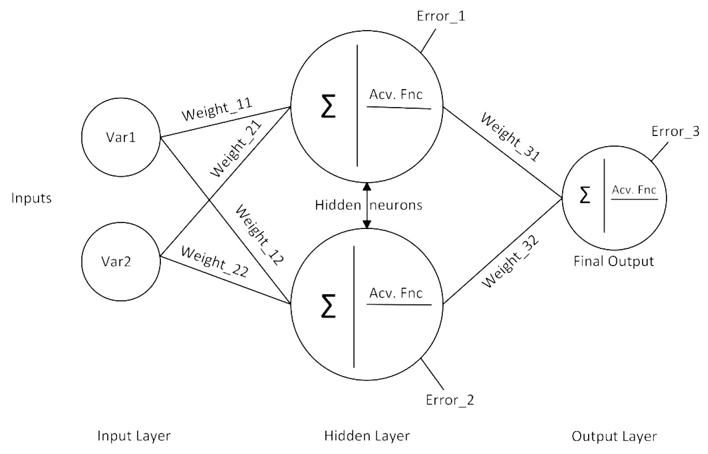
Overfitting is a serious problem for ANN models. If an ANN model having good fit in the training dataset fails in the testing dataset, it means that this model suffers extensively from the overfitting problem. In general, this problem is inevitable for ANN models having a small number of observations. On the other hand, if the number of parameters in an ANN model is higher than the number of observations, the ANN model does not adequately fit the training dataset ([34]). Because there was a total of 180 observations for each stand variable in this study, simple neural network models were implemented to prevent overfitting. The method of determining the number of parameters in an ANN model is shown in Fig. 2.
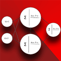
Fig. 2 - A simple representation of ANN model with one hidden layer with two hidden neurons (or nodes). This network includes a total of nine parameters (six weight and three error parameters).
Another way to avoid overfitting is to select a suitable regularization training function, such as the Levenberg-Marquardt, Bayesian, or variable learning rate gradient descent function. In this study, the Bayesian function was chosen because it can capture nonlinear patterns in the dataset and produce an S-shaped curve. This technique is also quite robust for overfitting ([40]).
As with the regression approach, the initial objective in an ANN model is to minimize errors (eqn. 7). This study aimed to minimize the mean of squared errors (also called the objective function). Different performance functions can be used as the objective function, such as the mean absolute error. In this study, the overall prediction performance of the ANN models was measured by the mean squared error, which is an indicator of the variation in the errors (eqn. 7):
where Oi is the measured target values, Pi is the predicted outputs, and n is the number of observations; D is a training data set, and M is a given network architecture.
In the Bayesian regularization technique, an additional term is added to the objective function (eqn. 8), and this allows the penalization of large weights and thereby improves the generalization ability of the ANN models ([15]).
where Ew is the sum of squared weights and α and β are the parameters of objective function (also called the regularization parameters).
The regularization parameters α and β are adaptively estimated for determining the best weights based on the Bayesian learning rule and, hence, minimizing the regularized objective function (eqn. 9):
where P (w | D, α, β, M), P (w | β, M) and P (w | α, M) are the posterior probability, the likelihood function, and the prior distribution for network weights, respectively. P (D | α, β, M) is a normalization factor for regularization parameters.
Choosing the best number of hidden neurons, learning rate, and momentum factor is important for enhancing the learning capacity of ANN models. When many hidden neurons are used, ANN models tend to memorize the problem but do not generalize the relationships between inputs and output. Conversely, if only a few hidden neurons are used, ANN models do not reflect the patterns of the dataset ([36]). While the learning rate controls the speed of learning, the momentum factor adjusts the current weight changes depending on the previous weight changes.
In order to achieve the optimum number of hidden neurons, learning rate, and momentum value, different combinations of these factors were studied. In this trial-and-error process, the number of hidden neurons varied from 2 to 10 and the learning rate and momentum factor varied from 0.1 to 0.9.
In this study, a total of 180 data items for each stand variable were used to evaluate the performance of the ANN models. To promote the performance of the ANN models and avoid overfitting, the five-fold cross-validation was employed using the entire dataset. The ANN models were conceived using the MATLAB® software ([31]). Inputs and output were the independent and dependent variables of the modified Gompertz function, respectively. Specifically, the inputs were: [1/SI, 1/SD, SI2, SD2, and 1/A], [ln(SI), 1/SD, SI2, SD2, and 1/A], and [1/SI, 1/SD, ln(SI), ln(SD) and 1/A] for outputs ln(G), ln(V) and ln(N), respectively. Due to the small number of observations, the entire dataset was used for training the ANN models in this study. Therefore, the suitability of the ANN models for the forest yield principles was assessed using the artificially generated data, which consisted of 150 years’ worth of simulation data divided into 10-year periods. Each site index class (i.e., 12, 22, and 32 m) included different stand density ratios (3, 5, 7, and 9; a stand density ratio of 9 means that the stand is fully stocked) and ages. After those new inputs were transformed based on the inputs of each ANN model, the testing process began.
Model evaluation
The statistical evaluation of the regression and ANN models was done using the adjusted coefficient of determination (Radj2, eqn. 10) and root mean square error (RMSE, eqn. 11):
where Oi is a measured value, Pi is a predicted value, Omean is a mean of the measured values, n is the number of measurements, and k is the number of coefficients (parameters for the ANN model). In calculating the Radj2 and RMSE, the inputs ln(V), ln(G), and ln(N) were back transformed to make the statistical evaluations more meaningful.
Results
The goodness-of-fit statistics, estimated coefficients, and t- and p-values of the nonlinear regression models developed for each stand variable are shown in Tab. 2. All of the coefficients estimated for SI, SD, and A and the other explanatory variables derived from SI, SD, and A were significant at the 5% level. The Radj2 values showed that the amounts of the variations explained by the nonlinear regression models (80% to 96%) were satisfactory for G, V, and N.
Tab. 2 - Coefficient estimates (with t- and p-values, and standard error, SE) and goodness-of-fit statistics of nonlinear regression models developed for predicting basal area (G, m2 ha-1), volume (V, m3 ha-1), and the number of trees (N, number ha-1) of Crimean pine stands.
| Model | Coefficient | Estimate | SE | t-value | p-value | R adj 2 | RMSE |
|---|---|---|---|---|---|---|---|
| G | b1 | 12.542 | 0.252 | 49.691 | <0.0001 | 0.96 | 3.24 |
| a1 | 1.926 | 0.18 | 10.726 | <0.0001 | |||
| a2 | 0.527 | 0.04 | 13.257 | <0.0001 | |||
| a3 | 0.00004 | 0 | 4.0689 | <0.0001 | |||
| a4 | -0.0005 | 0 | 9.7649 | <0.0001 | |||
| b3 | -21.846 | 2.471 | 8.8406 | <0.0001 | |||
| V | b1 | 19.732 | 0.808 | 24.412 | <0.0001 | 0.8 | 108.15 |
| a1 | 2.214 | 0.382 | 5.79 | <0.0001 | |||
| a2 | 0.129 | 0.054 | 2.4 | <0.0001 | |||
| a3 | 0.001 | 0.001 | 1.832 | <0.0001 | |||
| a4 | -0.005 | 0.001 | 3.916 | <0.0001 | |||
| b3 | -54.144 | 16.15 | 3.352 | <0.0001 | |||
| N | b1 | 9.565 | 0.427 | 22.388 | <0.0001 | 0.85 | 144.18 |
| a1 | 1.111 | 0.325 | 3.415 | <0.0001 | |||
| a2 | 0.662 | 0.165 | 4.004 | <0.0001 | |||
| a3 | 0.111 | 0.026 | 4.266 | <0.0001 | |||
| a4 | 0.34 | 0.058 | 5.857 | <0.0001 | |||
| b3 | 67.998 | 6.493 | 10.472 | <0.0001 |
The goodness-of-fit statistics and network parameters of the best ANN models for each stand variable are shown in Tab. 3. The ANN models successfully described the variations in G, V, and N (the Radj2 value ranged from 0.86 to 0.97). Therefore, we concluded that simple ANN models having one hidden layer with a small number of hidden neurons (n<10) were adequate for developing the variable-density yield models.
Tab. 3 - The number of parameters, learning rate, momentum, and goodness-of-fit statistics of ANN-based variable-density yield models developed for predicting basal area (G, m2 ha-1), volume (V, m3 ha-1), and stem number (N, number ha-1) of Crimean pine stands.
| Parameter | G | V | N |
|---|---|---|---|
| Number of inputs | 5 | 5 | 5 |
| Number of network parameters | 57 | 36 | 50 |
| Number of hidden neurons | 8 | 5 | 7 |
| Learning rate | 0.1 | 0.1 | 0.1 |
| Momentum value | 0.5 | 0.5 | 0.5 |
| R adj 2 | 0.97 | 0.97 | 0.86 |
| RMSE | 2.77 | 35.79 | 143.87 |
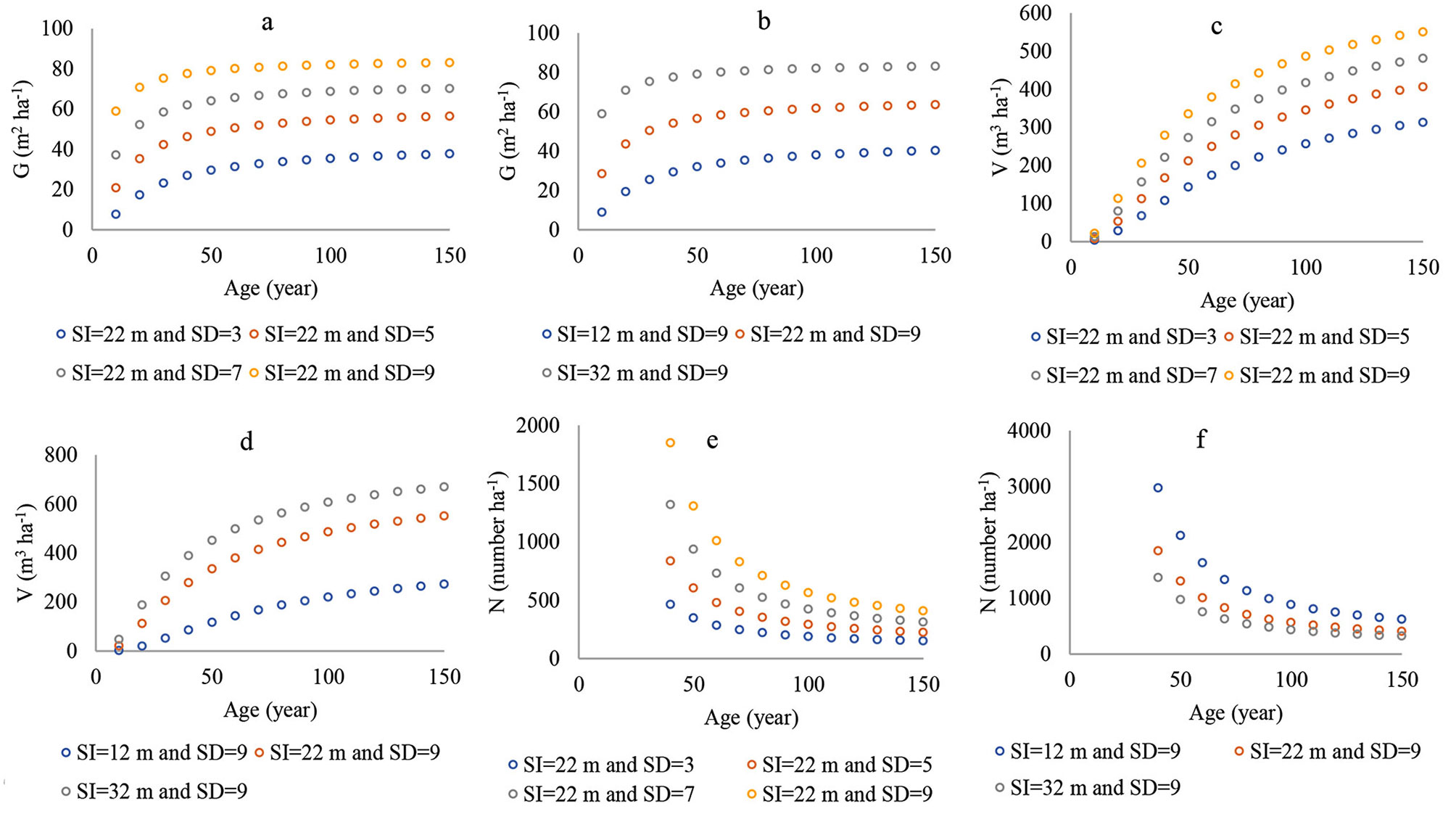
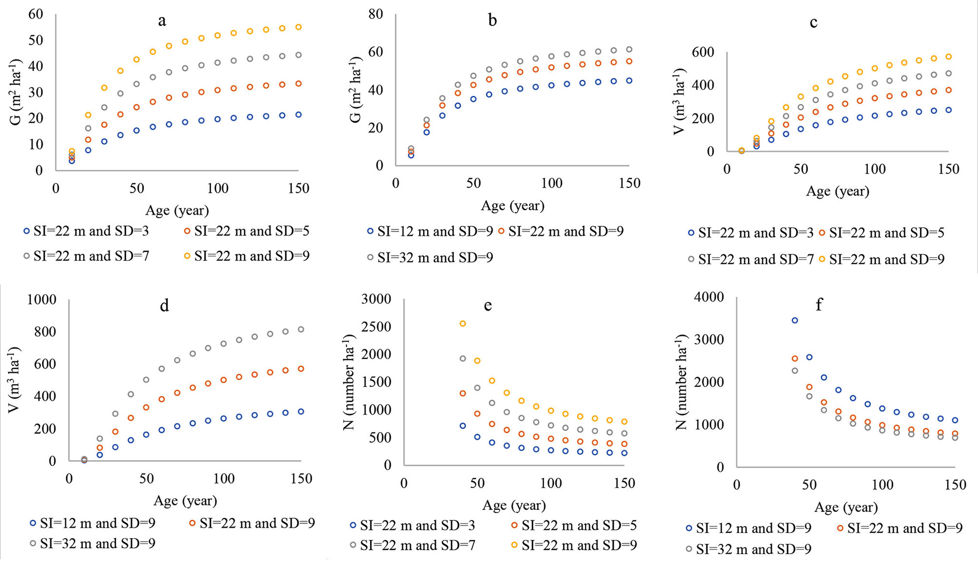
The number of parameters in the ANN models (namely, the coefficients for the regression models) was higher than for the nonlinear regression models. However, both of them provided a similar statistical performance for G and N. The ANN model was better than the regression model in predicting V. Similarly, both of them yielded polymorphic curves with a variable asymptote (Fig. 3a-f, Fig. 4a-f). These results were compatible with the principles of forest yield. In addition, it appeared that the ANN models were better for reflecting the patterns of G, V, and N when relying on SI and SD than the nonlinear regression models.
Fig. 3 - Curves of nonlinear regression models for (a) G, basal area, (c) V, stand volume, and (e) N, number of trees, based on different stand densities within same site index; (b) basal area, (d) stand volume, and (f) number of trees based on different site indexes within same stand density.
Fig. 4 - Curves of ANN models for (a) G, basal area, (c) V, stand volume, and (e) N, number of trees, based on different stand densities within same site index; (b) basal area, (d) volume and (f) the number of trees based on different site indexes within same stand density.
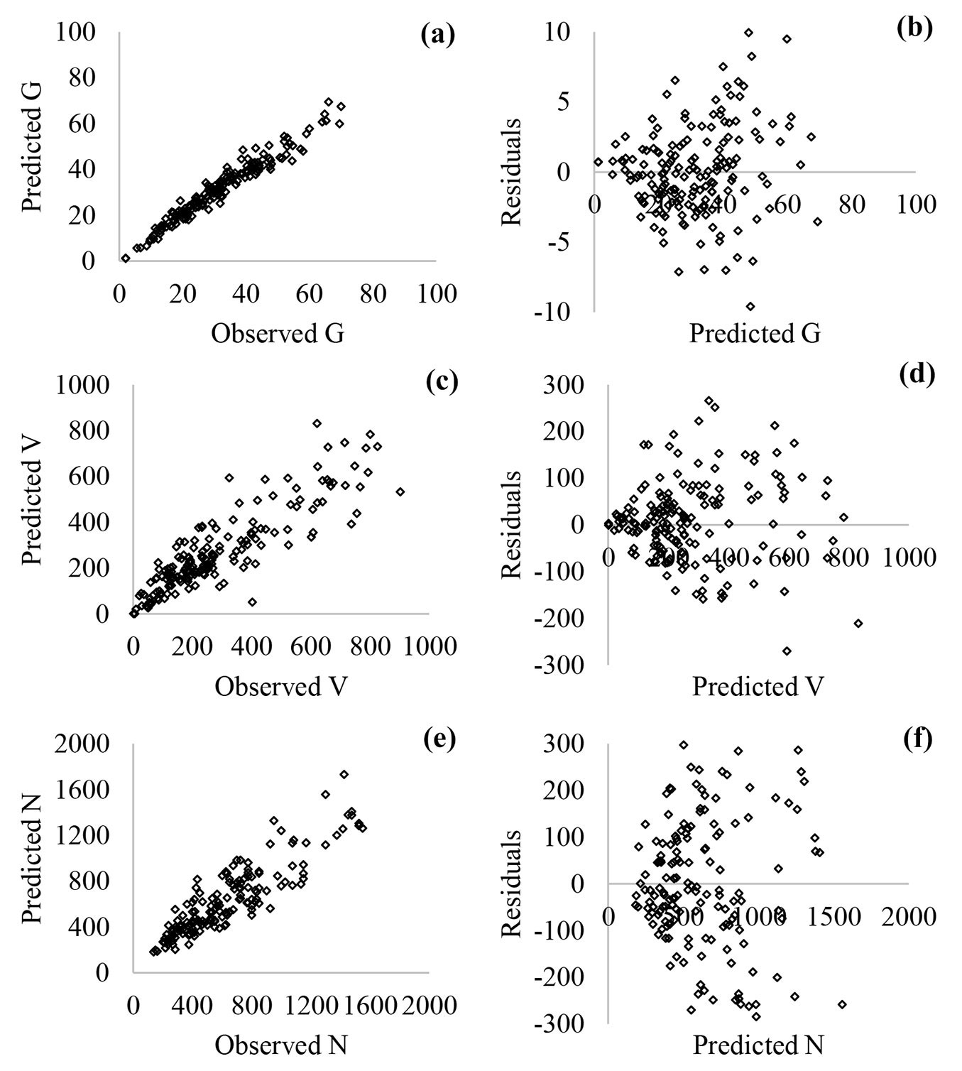
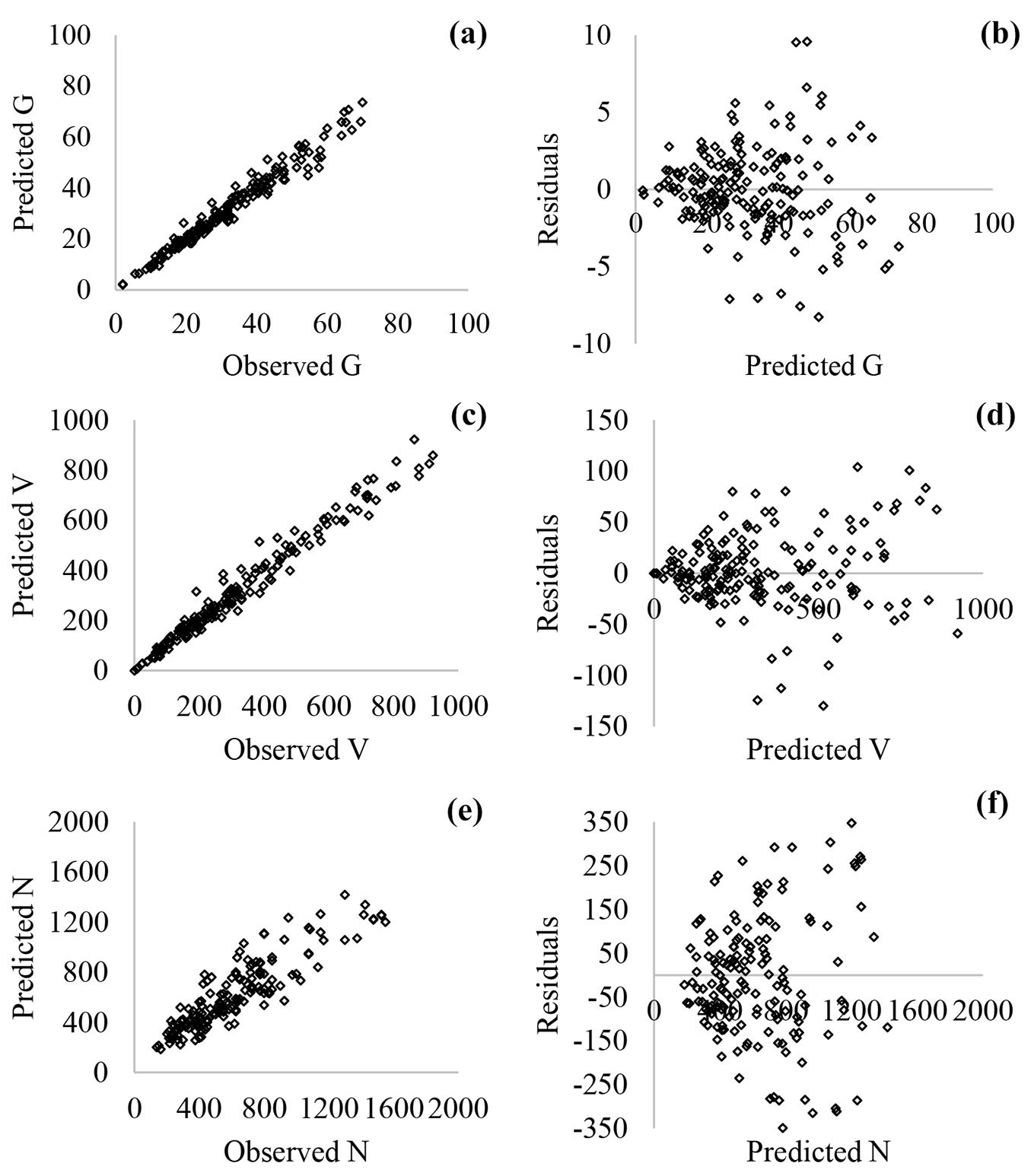
According to Fig. 5 and Fig. 6, the nonconstant variance in residuals of the nonlinear regression models was more prominent compared with the ANN models. In addition, both of the models had similar relationships between observed and predicted values (Fig. 5a, Fig. 5c, Fig. 5e and Fig. 6a, Fig. 6c, Fig. 6e).
Fig. 5 - Scatterplots of predicted vs. observed values (a: basal area, G; c: stand volume, V; e: number of trees, N) and residuals vs. predicted values (b: G; d: V; f: N) for nonlinear regression models.
Fig. 6 - Scatterplots of predicted vs. observed values (a: basal area, G; c: stand volume, V; e: the number of trees, N) and residuals vs. predicted values (b: G; d: V; f: N) for ANN models.
Discussion
In most studies using ANN models, the findings have been discussed only with the consideration of the goodness-of-fit statistics ([3], [26]). In forestry modeling, the principles of forest growth and yield are extremely important ([44]). Therefore, this study took into account both the goodness-of-fit statistics and the principles of forest yield and contrasted the ANN models accordingly. The ANN models developed showed reasonable statistical and biological behaviors in predicting G, V, and N. With this in mind, this study presented important findings for ANN modeling in forestry.
The Gompertz function was modified to develop the dynamic variable-density yield models in this study. The variables SI and SD were added to the growth-rate parameter of the Gompertz function, thereby the principles of forest yield could be met. A similar approach was used in the study of Temesgen et al. ([41]). In their study, the Chapman-Richards function was expanded to incorporate stand and tree variables to improve height predictions in forests with multiple species and multiple layers. Likewise, Fortin et al. ([16]) modified the von Bertalanffy-Richards function to satisfy the expected biological patterns of basal area growth of red spruce and balsam fir after logging treatments.
ANN models were more dynamic than nonlinear regression models in describing patterns of G, V, and N. This result is attributable to the nonlinear transfer function in the hidden layer of ANN models ([23]). Zhang et al. ([48]) demonstrated that ANN models facilitated the modeling of complex nonlinear relationships between tree growth and climate variables. Guan et al. ([20]) showed that the ANN model had great potential for constructing a dynamic model requiring a higher-order approximation.
Developing a dynamic nonlinear regression model can be difficult due to the difficulty in determining the starting values of the parameters ([13]). Developing an ANN model with many explanatory variables can be easier than developing a nonlinear regression model. On the other hand, the correlations among explanatory variables may affect the sign and magnitude of the regression parameters to be estimated and may result in unreasonable statistical and biological behaviors. Similarly, some irrelevant explanatory variables (inputs) may decrease the accuracy of ANN models or may induce small changes in their performance ([29]). Therefore, the selection of the variables is essential for both modeling approaches.
The accuracy of ANN models is highly dependent on the selection of network parameters ([30]). The choice of network parameters was reported in only a few studies. In the study of Liu & Zhang ([28]), while the learning rate was 0.3, the momentum was 0.7 in predicting the lumber volume, lumber value, chip volume, and total product value. In the study of Ozçelik et al. ([36]), the learning rate was 0.1 and the momentum was 0.3 in predicting the total tree heights. Castaño-Santamaría et al. ([6]) found that the best values for the learning rate and the momentum were 0.1 and 0.2, respectively, in predicting tree heights. Ozçelik et al. ([37]) found that the optimal values for the learning rate and the momentum were 0.1 and 0.3, respectively, in predicting tree stem volumes. In our study, the optimal learning rate and momentum were 0.1 and 0.5, respectively, in predicting the G, V, and N.
This study demonstrated that simple ANN models with one hidden layer and only a few hidden neurons (n<10) were adequate for accurately predicting the G, V, and N. These findings are compatible with the results of Castaño-Santamaría et al. ([6]), Liu & Zhang ([28]), and Ozçelik et al. ([36]), who reported that one hidden layer and a small number of hidden neurons were adequate for the prediction of forest attributes.
Conclusions
Many researchers paid attention to the goodness-of-fit statistics in evaluating ANN models and comparing ANN models with other modeling approaches. However, the biological rationales are often overlooked. This study showed that two different modeling approaches with similar error statistics may provide different curves depending on the SI and SD for G, V, and N. Therefore, it is recommended that both statistical and biological behaviors should be examined together when comparing different modeling approaches. In addition, we analyzed how the choice of network parameters affected the performance of ANN models. The best results were achieved using ANN models with one hidden layer and only a few hidden neurons. The Bayesian regularization training function with the tangent-sigmoid and linear activation functions at the hidden layer and the output layer, respectively, was suitable for meeting the principles of forest yield. The best learning rate and momentum were 0.1 and 0.5, respectively, for the prediction of G, V, and N. The knowledge obtained from this study can be a guideline for future similar studies.
List of abbreviations
A: Stand age; ANN: Artificial Neural Network; G: Basal area per hectare; N: The number of trees per hectare; SD: Stand density; SI: Site index; V: Stand volume per hectare
Acknowledgements
The authors thank the General Directorate of Forestry for the legal permission of field studies, as well as Dr. Sinan Bulut, forest engineer Ömer Bulut and Kutay Kaya for their help in collecting data.
Funding
This study was a part of a PhD thesis supported financially by the Scientific Research Project Unit of Çankiri Karatekin University, Turkey (grant: OF061218D05) and the Turkish Scientific and Technical Research Institute (TUBITAK, grant: TOVAG-119O061).
Author contributions
FB completed the statistical analyses and wrote the manuscript draft. IE and AG contributed to the idea, reviewed and edited the manuscript. All authors have read and approved the final manuscript.
References
Gscholar
Gscholar
Gscholar
CrossRef | Gscholar
Gscholar
Gscholar
Authors’ Info
Authors’ Affiliation
Ilker Ercanli 0000-0003-4250-7371
Alkan Günlü 0000-0002-6458-6165
Çankiri Karatekin University, Faculty of Forestry, 18200, Çankiri (Turkey)
Corresponding author
Paper Info
Citation
Bolat F, Ercanli I, Günlü A (2023). Yield of forests in Ankara Regional Directory of Forestry in Turkey: comparison of regression and artificial neural network models based on statistical and biological behaviors. iForest 16: 30-37. - doi: 10.3832/ifor4116-015
Academic Editor
Maurizio Marchi
Paper history
Received: Apr 14, 2022
Accepted: Nov 04, 2022
First online: Jan 22, 2023
Publication Date: Feb 28, 2023
Publication Time: 2.63 months
Copyright Information
© SISEF - The Italian Society of Silviculture and Forest Ecology 2023
Open Access
This article is distributed under the terms of the Creative Commons Attribution-Non Commercial 4.0 International (https://creativecommons.org/licenses/by-nc/4.0/), which permits unrestricted use, distribution, and reproduction in any medium, provided you give appropriate credit to the original author(s) and the source, provide a link to the Creative Commons license, and indicate if changes were made.
Web Metrics
Breakdown by View Type
Article Usage
Total Article Views: 26861
(from publication date up to now)
Breakdown by View Type
HTML Page Views: 21716
Abstract Page Views: 2697
PDF Downloads: 1946
Citation/Reference Downloads: 0
XML Downloads: 502
Web Metrics
Days since publication: 1207
Overall contacts: 26861
Avg. contacts per week: 155.78
Article Citations
Article citations are based on data periodically collected from the Clarivate Web of Science web site
(last update: Mar 2025)
Total number of cites (since 2023): 6
Average cites per year: 2.00
Publication Metrics
by Dimensions ©
Articles citing this article
List of the papers citing this article based on CrossRef Cited-by.
Related Contents
iForest Similar Articles
Short Communications
Estimation of canopy attributes of wild cacao trees using digital cover photography and machine learning algorithms
vol. 14, pp. 517-521 (online: 17 November 2021)
Research Articles
Estimation of above-ground biomass using machine learning approaches with InSAR and LiDAR data in tropical peat swamp forest of Brunei Darussalam
vol. 17, pp. 172-179 (online: 17 June 2024)
Research Articles
Forest fire occurrence modeling in Southwest Turkey using MaxEnt machine learning technique
vol. 17, pp. 10-18 (online: 02 February 2024)
Research Articles
Exploring machine learning modeling approaches for biomass and carbon dioxide weight estimation in Lebanon cedar trees
vol. 17, pp. 19-28 (online: 12 February 2024)
Research Articles
Prediction of stem diameter and biomass at individual tree crown level with advanced machine learning techniques
vol. 12, pp. 323-329 (online: 14 June 2019)
Research Articles
Classification of xeric scrub forest species using machine learning and optical and LiDAR drone data capture
vol. 18, pp. 357-365 (online: 07 December 2025)
Research Articles
Above ground biomass estimation from UAV high resolution RGB images and LiDAR data in a pine forest in Southern Italy
vol. 15, pp. 451-457 (online: 03 November 2022)
Research Articles
Validation of visual and machine strength grading for Italian beech with additional sampling
vol. 14, pp. 260-267 (online: 29 May 2021)
Research Articles
Local ecological niche modelling to provide suitability maps for 27 forest tree species in edge conditions
vol. 13, pp. 230-237 (online: 19 June 2020)
Research Articles
Bayesian geographically weighted regression and its application for local modeling of relationships between tree variables
vol. 11, pp. 542-552 (online: 01 September 2018)
iForest Database Search
Search By Author
Search By Keyword
Google Scholar Search
Citing Articles
Search By Author
Search By Keywords
PubMed Search
Search By Author
Search By Keyword

