Bayesian geographically weighted regression and its application for local modeling of relationships between tree variables
iForest - Biogeosciences and Forestry, Volume 11, Issue 5, Pages 542-552 (2018)
doi: https://doi.org/10.3832/ifor2574-011
Published: Sep 01, 2018 - Copyright © 2018 SISEF
Research Articles
Abstract
Geographically weighted regression (GWR) has become popular in recent years to deal with spatial autocorrelation and heterogeneity in forestry and ecological data. However, researchers have realized that GWR has some limitations, such as correlated model coefficients across study areas, strong influence of outliers, weak data problem, etc. In this study, we applied Bayesian geographically weighted regression (BGWR) and a robust BGWR (rBGWR) to model the relationship between tree crown and diameter using observed tree data and simulated data to investigate model fitting and performance in order to overcome some limitations of GWR. Our results indicated that, for observed tree data, the rBGWR estimated tree crown more accurate than both BGWR and GWR. For the simulated data, 74.1% of the estimated slope coefficients by rBGWR and 73.4% of the estimated slope coefficients by BGWR were not significantly different (α = 0.05) from the corresponding simulated slope coefficients. The estimation of model coefficients by rBGWR was not sensitive to outliers, but the coefficient estimation by GWR was strongly affected by those outliers. The majority of the coefficient estimates by rBGWR and BGWR for weak observations were not significantly (α = 0.05) different from the simulated coefficients. Therefore, BGWR (including rBGWR) may be a better alternative to overcome some limitations of GWR. In addition, both BGWR and rBGWR were more powerful than GWR to detect the spatial areas with non-constant variance or spatial outliers.
Keywords
Spatial Autocorrelation, Spatial Heterogeneity, Robust Regression, Spatially Varying Coefficients Models
Introduction
Most tree or plant communities display some degree of spatial structure in the form of geographical patchiness or gradients. Trees or plants at close distances interact to each other (e.g., by competition) more than those farther away ([24], [25], [12]). In forestry, young stands commonly exhibit positive spatial autocorrelation due to micro-site patchiness, whereas the competition among trees promotes negative spatial autocorrelation ([43], [14]). In addition, spatial effects (i.e., spatial autocorrelation and heterogeneity) in tree or plant communities may exist at multiple spatial scales and for many variables ([51], [28], [37], [38]). Thus, incorporating spatial effects into statistical data analysis and modeling requires creative approaches to describe real-world systems ([21]). In the last decade, researchers are increasingly interested in understanding the causes and consequences of spatial autocorrelation and heterogeneity in ecosystem functions ([33]).
When spatial autocorrelation and heterogeneity exist in forestry and ecological data, the independence and homogeneity assumptions of traditional statistical methods, e.g., ordinary least squares (OLS), may be violated ([21]). In recent years, different spatial models have been developed to deal with spatial effects in the relationships between variables. Based on the spatial scales used in the modeling process, spatial models can be categorized into global and local models ([23], [44], [32]). Global models, such as linear mixed models and spatial autoregressive models ([55], [40]), assume that spatial variation is the same everywhere. Thus, a single model is developed using the whole data set and is used for the entire study area. Commonly, a global model requires a device to model spatial autocorrelation among observations in neighboring locations, through either a covariance matrix that can be estimated using a variogram or spatial weight matrix based on spatial proximity of neighbors ([34], [35], [36]). Obviously, global models do not well represent spatial variations at any individual location and may not be effective to deal with spatial heterogeneity.
In contrast, local models, such as geographically weighted regression (GWR), fit a regression relationship for each spatial location using the neighbors within a given bandwidth ([13]). In recent years, GWR has been applied in various disciplines, including ecology, forestry, real estate, and healthcare ([39], [11], [53], [30]). Local models are more useful to explore locational spatial variation (heterogeneity) in the relationships between variables. In forestry and ecological studies, local models can be a useful tool for evaluating, testing, and modeling the influence of micro-site variation, competition status, growth potential, and management activities on trees or plants. Further, these local model coefficients and model fitting statistics can be readily displayed using GIS or graphic packages to explore local “hot” or “cold” spots across the study area ([53]).
However, researchers have realized that GWR has several limitations: (i) lack of a unifying approach to estimate local coefficients; (ii) incorrect estimates of dispersion of model coefficients, as GWR utilizes the same sample data observations (with different spatial weights) to produce a sequence of parameter estimates for all locations in the space. Consequently, the estimated model coefficients are dependent across spatial locations, and the correct expression for the variance of local coefficients could be non-linear; (iii) the influence of outliers (i.e., unusual data observations on Y-axis), because local coefficient estimates can be strongly affected by a single outlier; (iv) weak data (i.e., any observation with insufficient neighbors within its effective bandwidth) problem, especially if the “pre-selected” bandwidth is small; and (v) assumption violation of homogeneous error variance ([27], [50]).
To overcome the limitations of GWR, a Bayesian approach was proposed to estimate the local regression coefficients, namely Bayesian geographically weighted regression (BGWR - [26], [27]). BGWR introduced the concept of parameter smoothing, which polls the strength among observations. In other words, parameter smoothing defines the relationship between the local regression coefficients of a subject location and the local coefficients of other locations in the study area. Further, a robust BGWR (rBGWR) was also introduced to deal with problems in data such as outliers and weak data ([26], [27]).
However, BGWR requires the use of Gibbs sampler, a Monte Carlo simulation, to estimate its parameters. The Gibbs sampler ([18], [17]) is one of the most frequently used methods of Markov Chain Monte Carlo (MCMC). It generates random samples from a (marginal) probability distribution indirectly, without the need to calculate the density itself. By simulating a large enough sample, the sample characteristics such as mean and variance can be computed to the desirable degree of accuracy ([5], [2]). Gelfand & Smith ([18]) demonstrated how such methods can be useful for a variety of Bayesian inference problems.
To date, limited studies have used the BGWR methods. LeSage ([27]) compared GWR and BGWR with econometric data. Furutani ([15]) used BGWR to study land prices in Yokohama, Japan. Similarly, Clifton & Romero-Barrutieta ([6]) used BGWR to study the role of geography and institutions on growth and development for a region of the United States. However, we are not aware of any applications of BGWR in the fields of ecology or forestry. The objectives of this study were to: (i) fit a relationship between tree crown area and diameter at breast height (dbh) for observed data and simulated data using GWR, BGWR, and rBGWR; (ii) compare model fitting and performance of the three modeling methods; and (iii) investigate the usefulness, advantages, and limitations of BGWR and rBGWR in handling outliers and weak data problems.
Theoretical background
Geographically weighted regression
A linear regression relationship between variables can be expressed as (eqn. 1):
where Y is an n × 1 vector of the response variable, X is an n × p matrix with a (first) column of one and (p - 1) explanatory variables, β is a p × 1 vector of model coefficients, and ε is an n × 1 vector of random error term with i.i.d. N(0, σ2I), where I denotes an n × n identity matrix. Traditionally, the relationship represented by eqn. 1 is assumed to be universal or constant across the geographical study area.
Now suppose that we have a set of locations si (i = 1, 2, …, n) with geographic coordinates. The underlying model for geographically weighted regression (GWR) can be expressed as (eqn. 2):
where Y and X are defined as in eqn. 1, W(si) is an n × n diagonal matrix of spatial weight, β(si) is a p × 1 vector of model coefficients associated with the subject location si, and ε(si) is an n × 1 vector of random error term with i.i.d. N(0, σ2I) associated with the subject location si. The aim of GWR is to obtain non-parametric estimates of the regression model for each geographical location si. This can be achieved by using neighboring observations near location si as follows: (i) find a point at one particular location si; (ii) compute the distance-based spatial weight matrix W(si); and (iii) estimate the model coefficients using weighted least-squares regression ([3], [13] - eqn. 3):
where T is the transposed matrix and the other terms are as defined above. Further, using the analogies of local information matrix and hat matrix, Fotheringham et al. ([13]) gave the following expression to compute the asymptotic variance of β(si)(eqn. 4):
where H(si) = [X(si)T W(si) X(si)] -1 X(si)T W(si). Unfortunately, this expression is incorrect for variance of local coefficients ([27], [50]).
The spatial weight matrix W(si) is a function of the distance between the subject location (si) and neighboring observations (sj), and determines the influence of the neighbors on the parameter estimation of local regression coefficients. Three weight functions are commonly used to compute the spatial weight matrix, including Gaussian, exponential, and bi-square weight functions ([13]). The bandwidth of the weight function is either fixed (i.e., Gaussian and exponential functions) or variable (i.e., bi-square function - [22]). The “optimal” bandwidth can be determined using the cross-validation (CV) method, the Akaike’s information criterion (AIC) or pre-defined by the researcher ([10]).
Bayesian geographically weighted regression
The underlying model of Bayesian geographically weighted regression (BGWR) is the same as that of GWR in eqn. 2. However, the model error term ε(si) assumes to follow i.i.d. N (0, σ2V(si)), where V (si) = diag (vs-i1 , vs-i2 , …, vs-in ) is an n × n diagonal matrix. Basically, V(si) represents a set of non-constant variances across space and needs to be estimated from the data. BGWR requires the use of a parameter smoothing specification, which is a mathematical function representing the relationship among spatially varying coefficients. For example, a distance smoothing parameter specification is as follows (eqn. 5):
where ws-ij represents normalized distance-based spatial weights, i.e., sum of row vector (ws-i1, ..., ws-in) is unity and assumes ws-ij = 0. The stochastic variation term υ(si) follows N[0, σ(si)2 δ2 (X(si)T W(si) X(si))-1] . Note the variance of υ(si) contains a scale factor δ2 which quantifies the amount of variation among the local coefficient vector β(si). The role of this scale factor in estimating local parameters will be discussed later.
The parameter smoothing function and assumption of heterogeneous variance ensure that BGWR captures spatial heterogeneity and autocorrelation. On the other hand, these assumptions add complexity to the modeling process. Thus, a Bayesian approach is required to estimate the mod-el coefficients. The likelihood of BGWR ([27]) can be represented as (eqn. 6):
where Y = W(si) Y(si), X(si) = W(si) X(si), J(si) = (wi1 × Ip, ..., win × Ip) and γT = β(si), ..., β(sn). Note that when V(si) = In, and δ = ∞, both X(si)T X(si)/δ2 and X(si)T X(si) J(si)γ/δ2 are zero and the BGWR model is reduced to the GWR model.
Using eqn. 6 and the distribution of υ(si), the conditional distribution of β(si), given δ, σ(si), V(si), and γ, is a multivariate normal and can be expressed as (eqn. 7):
where δ, σ(si) and V(si), are hyper-parameters (i.e., the parameters of prior distributions), and γ represents the value of other βÌ(si) for observations j≠i. Geweke ([19]) proved the existence of the posterior density and moments of this model.
Choosing a prior distribution or prior information for the hyper-parameters is an important issue in Bayesian inference, as it may be sensitive or robust to the choice of the prior distribution ([7]). In this study, the conditional prior distributions of the BGWR hyper-parameters (i.e., δ, σ(si) and V(si)) are as follows:
(1) The conditional prior distribution of scale factor δ (eqn. 8):
where a and b are the Gamma distribution parameters. The mean and variance of the Gamma distribution are a/b and a/b2, respectively. Alternatively, the conditional prior distribution of δ is χ2(np), such that (eqn. 9):
Note that the value of δ is very important for defining the relation of β(si) with other neighboring β(sj), j≠i. When the inherent dispersion of the GWR parameters is large for a given data set, it will require a larger δ value to fit BGWR ([27]). A very small value of δ imposes the constraints on the variation of parameters β(si), and it becomes a distance-weighted linear combination of neighboring β(sj). In contrast, a larger value of δ allows the parameter β(si) to be estimated from the data and less influenced by other neighboring β(sj). As a result, an informative prior for δ is chosen in this study. It can be estimated using an empirical Bayes method ([4]). Once the estimate is obtained, we can choose a set of values of δ (e.g., multiply by some constants such as 0.1, 0.25 and 0.5) to explore the interaction of the scale factor with the variation of estimated local coefficients.
(2) The conditional prior distribution of σ(si) (eqn. 10):
where ε(si) = Y(si) - X(si) β(si), and m denotes the number of observations with non-negligible weights. Hence, the posterior distribution of σ(si) is χ2(m). It is a squared sum of m independent variables with standard normal distributions.
(3) The conditional prior distribution of V(si) (eqn. 11):
where r is a hyper-parameter that controls the amount of dispersion in the V(si) estimates across the observations. This type of prior has been used previously ([31], [19], [26]). The motivation for assigning this prior to V(si) is that the mean of prior equals unity and the prior variance is 2/r ([27]). Thus, introduction of a single hyper-parameter r can generate n2 parameter estimates. However, in order to constrain V(si) in relation to ε(si) and σ(si), the following conditional distribution is used to generate the posterior samples of V(si) (eqn. 12):
which provides greater flexibility to vij (the jth diagonal of V(si)), depending on how close the prediction for the jth observation was while calibrating the local parameters for the ith subject location.
Given the likelihood function and the conditional prior distributions of BGWR hyper-parameters, the posterior distribution of βÌ(si) is simulated using the Gibbs sampler ([17]). As there are a large number of parameters in each draw (iteration), two approaches can be adopted to simulate the model parameters. In the first approach, the parameters are estimated sequentially for each observation in each simulation draw, and it will be computationally very expensive. In the second approach, the parameters are individually simulated across all draws (iterations) for every observation. One limitation of this approach is that there will be no parameter smoothing relationship. However, a robust parameter estimation (i.e., insensitive to outliers) can be implemented by this approach. The rBGWR uses an independent Student-t linear model, and the parameter estimation is powerful enough to handle outliers and to address robustness concerns in practical settings ([19]). In addition, this approach is computationally very efficient. Hereafter, this simplified Gibbs sampling approach with robust parameter estimation will be referred to as rBGWR.
Data and methods
We briefly discuss the observed data and simulated data, crown area regression model, model fitting process for each method (GWR, BGWR, and rBGWR), and the evaluation of the three methods.
Ontario softwood data
The observed data used in this study were a subset of the stem map data of a mature, second growth, uneven-aged softwood stand located near Sault Ste. Marie, Ontario, Canada ([9]). It was 150 × 200 m in size and had a total of 1698 trees. The dominant tree species included balsam fir (Abies balsamea [L.] Mill. - 57.6% in number of trees), black spruce (Picea mariana [Mill.] BSP. - 33.5%), and white spruce (Picea glauca [Moench.] Voss. - 4.6%). Other tree species were in smaller percentages and included white pine (Pinus strobus L.), balsam poplar (Populus balsamifera L.), Tamarack (Larix laricina [Du Roi] K. Koch), and white birch (Betula papyrifera Marsh.). The information on measurements included tree location (coordinate), diameter at breast height (dbh), total height, and crown area (crown) for trees dbh > 8.9 cm ([54], [55]).
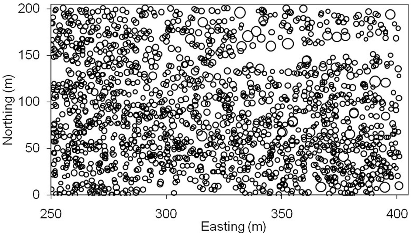
Tab. 1 shows the descriptive statistics of tree dbh and crown, as well as their spatial autocorrelation (Moran’s I), relative spatial heterogeneity (SH%), and nearest-neighbor distance ([54], [55]). Fig. 1 illustrates the stem map of trees with circle size proportional to the tree dbh. Note that the Ontario softwood data had some special features: (i) clustered spatial pattern of trees; (ii) large variation in tree dbh (e.g., potential outliers); and (iii) large gaps between trees in the upper portion of the plot (e.g., potential weak data observations).
Tab. 1 - Descriptive statistics of observed tree data (Ontario softwood stand). Moran’s I and SH% were calculated at lag distance of 4.48 m and 2.24 m, respectively.
| Variable | n | Mean | SD | Min | Max | Moran’s I | SH% | Distance (m) |
|---|---|---|---|---|---|---|---|---|
| dbh (cm) | 1698 | 18.68 | 8.47 | 11.43 | 84.07 | 0.087 | 91.64 | 2.2 (0.3-11.0) |
| Crown area (m2) | 1698 | 7.79 | 7.80 | 0.93 | 90.48 | 0.115 | 80.62 | - |
Fig. 1 - Map of tree locations for Ontario softwood data. Circles are proportional to the diameter at breast height of trees.
Regression model
Based on the relationship between tree dbh and crown in the data, we chose the following linear regression model (eqn. 13):
where crown is the tree crown area (m2), dbh is tree diameter at breast height (cm), β0 and β1 are regression coefficients to be estimated, ln is the natural logarithm, and ε is the model random error. The crown-dbh relationship was used in this study because crown is considered the “engine” of a tree, but it is difficult and time consuming to be measured in field. However, we emphasize that we did not intend to develop a predictive crown-dbh model. Rather, we attempted to demonstrate that BGWR is a flexible alternative modeling approach which can be used to investigate spatial heterogeneity in the relationships between response variable (tree crown) and covariate (dbh).
Simulated data
To objectively verify the performance of BGWR, a simulated tree data set with geographic coordinates, tree dbh and crown area, and known local regression coefficients was generated for each tree. The procedure of generating the simulated data is as follows:
(1) The AMORPHYS software ([46]) was used to generate tree locations with a clustered spatial pattern. The clustered spatial pattern was chosen because local models such as GWR would have more advantages over global models than random or regular spatial patterns ([55]). Then, the values of tree dbh were randomly generated from a two-parameter Weibull distribution, and other tree attributes such as tree crown area were calculated using a process-based stand model ([46]).
(2) The generated tree data were used to fit eqn. 13 by GWR 3.0 ([13]) to obtain the two local regression coefficients (β0 and β1) for each tree / location. These local regression coefficients were transformed into a unit scale [0, 1], and used to calculate the cumulative distribution function. The purpose of this step was to estimate the scale-invariant measure of association between β0 and β1 using a bivariate Gaussian copula ([41], [49]).
(3) Given the estimated association between β0 and β1, the bivariate Gaussian copula was used to randomly simulate the two coefficients (β0 and β1) in a unit scale [0, 1], and then transform these coefficients back to the original scale and assign the coefficients to the spatial locations generated in step (1).
(4) Create 5 outliers by artificially making the β1 coefficient very large (e.g., two times larger). Create scenarios of weak data (any observation with insufficient neighbors within its effective bandwidth) by deleting a few trees at the locations of low trees density.
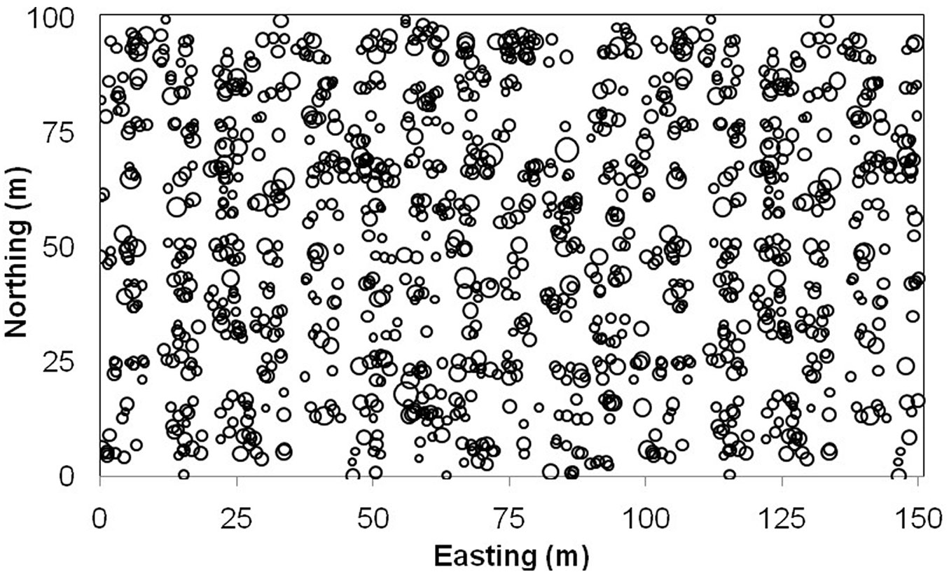
(5) Given the randomly generated regression coefficients (β0 and β1) and tree dbh generated in step (1), tree crown area was computed using eqn. 13 for each tree / location. Finally, a total of 1230 trees were simulated with geographic coordinates, tree dbh and crown, and known local regression coefficients for each location. Tab. 2 provides a summary of the simulated data. Fig. 2 illustrates the spatial pattern of these simulated trees with circle size proportional to tree dbh.
Tab. 2 - Descriptive statistics of simulated tree data (n=1230).
| Variable | Mean | SD | Min | Max | Moran’s I | SH% |
|---|---|---|---|---|---|---|
| DBH (cm) | 18.23 | 9.44 | 7.43 | 80.45 | 0.03 | 86.40 |
| Crown area (m2) | 12.94 | 7.00 | 4.61 | 74.91 | 0.05 | 86.90 |
| Intercept β0 | 0.201 | 0.143 | -0.260 | 0.580 | 0.01 | 87.80 |
| Slope β1 | 0.807 | 0.130 | 0.600 | 1.233 | 0.01 | 92.60 |
| Nearest neighbor distance | 1.4 | 1.26 | 0.15 | 6.47 | - | - |
Fig. 2 - Map of tree locations for simulated data. Circles are proportional to the diameter at breast height of trees.
Model fitting
Three modeling methods, GWR, BGWR, and rBGWR, were used to fit the linear relationship between ln(crown) and ln(dbh) (eqn. 13) for both Ontario softwood data and simulated data. The GWR model was fitted using GWR 3.0 software ([13]). The cross validation (CV) method was used to compare three spatial weigh functions, i.e., Gaussian (fixed kernel), exponential (fixed kernel), and tri-cube functions ([10]). In this study, the same Gaussian spatial weight function (fixed kernel) and bandwidth (10 m) were used for all three methods in order to make compatible model comparison ([13], [22]).
The BGWR and rBGWR models were fitted using bgwr.m and bgwrv.m Matlab functions available in the Econometric Toolbox ([26]). These functions were modified to accommodate the options of thinning for longer MCMC chains and calculation of deviance. Both BGWR methods require the prior distributions for the hyper-parameter r (related to V(si)) and the scale factor δ2. In this study, three priors (4, 5 and 6) were chosen for the hyper-parameter r. For each r, three priors on the scale factor δ2 were selected for the BGWR method, which were 10%, 25% and 50% of estimated using the empirical Bayes method with the sample data. The priors on these scale factors larger than 50% of the diffuse prior were not included, because larger priors reduce the efficacy of parameter smoothing and result in BGWR coefficients similar to GWR coefficients ([27]). Hence, there were nine BGWR models with three priors of r combined by three priors of δ2. However, the rBGWR models used only three priors of r.
Posterior distributions of model parameters for each model were sampled using the Gibbs sampler. A single long chain of MCMC was used to generate samples of each coefficient. The convergence of sampled coefficients was diagnosed using the method of Raftery & Lewis ([42]) and other exploratory tools. The convergence diagnostic suggested that most of the coefficients estimated by BGWR converged within 4000 samples after a sufficient burn in. However, those estimated coefficients with specification of smaller priors on the scale factor required almost 15.000 samples to converge at the precision of 0.005 (quartile = 0.025 and probability = 0.95).
Using the post convergence values of model coefficients, the Deviance Information Criterion (DIC - [45]) was calculated for all the models as an assessment measure of model fitting, such that DIC = D(β) +pD, where D(β) is the average deviance of the mean of posterior model coefficients, and pD is the effective number of model coefficients, which describes the complexity of the model and serves as a penalization term that corrects deviance’s propensity toward models with more parameters. Therefore, DIC is a Bayesian alternative to Akaike’s information criterion (AIC). A model with a smaller DIC value is desirable suggesting improved model fitting without excessive parameterization. In order to compare against GWR, one BGWR model and one rBGWR model with the smallest DIC value were chosen among all fitted models.
Model evaluation
The local coefficients estimated by the three methods (GWR, BGWR, and rBGWR) were summarized using descriptive statistics. For the Ontario softwood data, the two regression coefficients estimated by each method were interpolated using inverse distance weighting method and contour maps of these coefficients were generated for each method. Further, the model residuals from each method were assessed across a range of the explanatory variable (dbh).
The local regression coefficients were also evaluated for spatial heterogeneity using intra-block variance (Vintra) and inter-block variance (Vinter - [29], [16], [55]) as defined below (eqn. 14, eqn. 15):
where B is the number of blocks, ni is the number of observations in the ith block, and βij, βi, and β are the estimated local coefficients for jth observation in the ith block, the mean value of local coefficients in the ith block, and the overall mean of coefficients of the whole plot, respectively. In general, Vinter indicates the regional spatial variability, while Vintra quantifies the local spatial variability ([55]). These measures of spatial heterogeneity were compared among the three modeling methods for the Ontario softwood data.
For the simulated data, the “true” local coefficients of each observation were known. Hence, the 95% of credible limits for each coefficient estimated by BGWR and rBGWR were compared with the corresponding known coefficients for each location. If the 95% credible limits of the posterior samples of a coefficient estimated for a particular location included the known coefficient, the coefficient estimated by the method for the location was declared to be unbiased. The percentages of unbiased intercept, slope, and both (intercept and slope) coefficients for all locations by BGWR and rBGWR were calculated. However, this assessment was not used for GWR because the estimation of variance of local coefficients was incorrect ([27], [50]). Similarly, the estimation bias (defined as simulated-estimated) was computed for the two local coefficients as well as the response variable [ln(crown)] for each location and each modeling method.
Model fitting and performance were evaluated for special cases such as outliers and weak data (any observation with insufficient neighbors within its effective bandwidth) by comparing the estimated coefficients and predicted crown area by each modeling method. For the Ontario softwood data, the comparison was only for weak observations (no obvious outliers in the data), while for simulated data, the modeling fitting and performance were evaluated for both outliers and weak observations in terms of the 95% credible limits interval of the corresponding BGWR and rBGWR coefficients, and the estimation bias of model coefficients and tree crown area.
Results
Ontario softwood data
Model fitting
The identification of the “best” BGWR and rBGWR models for different priors of the hyper-parameters r and δ2 represented the first step of this study. Tab. 3 shows the model fitting statistics of the nine BGWR models (with the combination of three priors of r (4, 5, and 6) and three priors of δ2 (10%, 25% and 50% of the estimated δ2 by the empirical Bayes method from the data), as well as the three rBGWR models (for three priors of r 4, 5, and 6). The model deviances D(β), which measured model fitting, were very similar across the three priors of scale factors δ2 within a particular prior of r. However, the model complexity (pD) decreased as the prior of scale factor δ2 increased. Thus, the smallest DIC values were observed for the BGWR models at the scale factor δ2 = 50% across the three priors of r. This finding implies that the observed tree data favored a larger dispersion of local regression coefficients, and consequently it indicates the evidence of spatial heterogeneity in the sample data.
Tab. 3 - Model fitting statistics of nine BGWR models and three rBGWR models for the Ontario softwood data.
| Method | Model | Prior Mean of r |
Scale Factorδ2 (%) |
DIC | D(β) | pD |
|---|---|---|---|---|---|---|
| BGWR | 1 | 4 | 10 | 4183.1 | 893.9 | 3289.2 |
| 2 | 4 | 25 | 4149.6 | 899.7 | 3249.9 | |
| 3 | 4 | 50 | 4115.8 | 904.0 | 3211.8 | |
| 4 | 5 | 10 | 3891.4 | 1039.6 | 2851.8 | |
| 5 | 5 | 25 | 3852.6 | 1042.2 | 2810.3 | |
| 6 | 5 | 50 | 3826.7 | 1044.2 | 2782.5 | |
| 7 | 6 | 10 | 4516.4 | 1160.0 | 3356.4 | |
| 8 | 6 | 25 | 4500.0 | 1160.3 | 3339.7 | |
| 9 | 6 | 50 | 3751.1 | 1161.1 | 2590.1 | |
| rBGWR | 1 | 4 | - | 4620.2 | 1279.2 | 3341.1 |
| 2 | 5 | - | 4193.0 | 1307.0 | 2886.0 | |
| 3 | 6 | - | 5273.4 | 1323.7 | 3949.7 |
Interestingly, the BGWR and rBGWR models had consistently smaller DIC values for r = 5, which was consistent with the finding previously reported by LeSage ([27]). Therefore, the BGWR models with r = 5 and δ2 = 50% and the rBGWR models with r = 5 had the smallest DIC value, which were chosen to compare with the GWR model. While the model fitting statistics similar to D(β) and pD were also available for GWR, these values were not directly comparable ([48]). Thus, they were not reported for GWR. The coefficient of determination for the GWR model was 0.7824.
Tab. 4 compares the local regression coefficients estimated by GWR with the posterior means of local coefficients estimated by BGWR and rBGWR. It appears that the three modeling methods produced very similar mean and median values for the two coefficients (β0 and β1). But the rBGWR model yielded the largest variation for the two coefficients (the largest standard deviations and ranges), followed by the BGWR model, while the GWR had much smaller variation for the two coefficients (Tab. 4). The distributions of the intercept coefficient (β0) were positively skewed and the distributions of the slope coefficient (β1) were negatively skewed. Both were leptokurtic (kurtosis > 4.8) for the three modeling methods.
Tab. 4 - Summary of local regression coefficients by the three modeling methods (Ontario softwood data).
| Coefficient | Method | n | Mean | Median | SD | Skewness | Kurtosis | Min | Max |
|---|---|---|---|---|---|---|---|---|---|
| Intercept β0 | GWR | 1698 | -2.258 | -2.293 | 1.245 | 0.541 | 4.845 | -6.087 | 3.672 |
| BGWR | 1698 | -2.250 | -2.225 | 1.407 | 0.231 | 4.877 | -8.395 | 5.098 | |
| rBGWR | 1698 | -2.242 | -2.212 | 1.480 | 0.227 | 4.942 | -8.665 | 5.384 | |
| Slope β1 | GWR | 1698 | 1.426 | 1.440 | 0.424 | -0.596 | 4.845 | -0.736 | 2.774 |
| BGWR | 1698 | 1.428 | 1.425 | 0.482 | -0.252 | 4.877 | -1.113 | 3.485 | |
| rBGWR | 1698 | 1.426 | 1.421 | 0.507 | -0.255 | 4.942 | -1.216 | 3.576 |
Model prediction
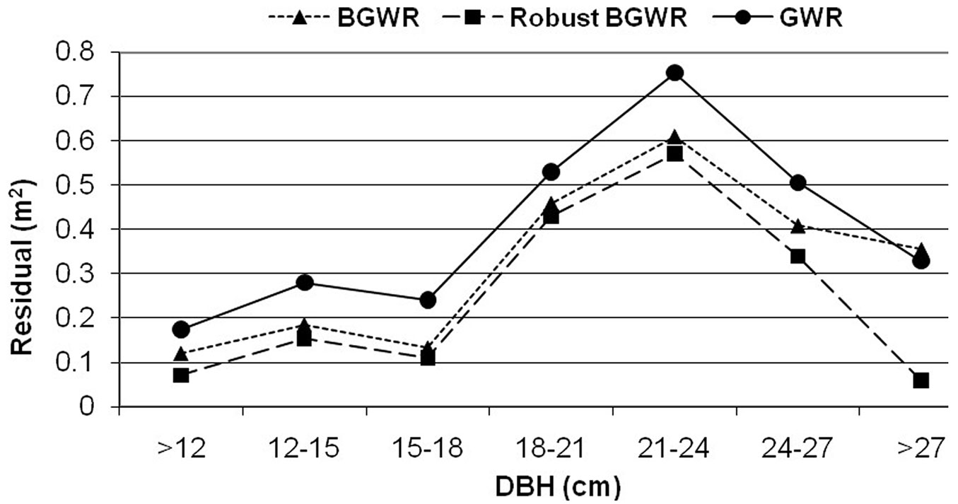
Fig. 3 illustrates the average prediction errors [= observed ln(crown) - predicted ln(crown)] from the three modeling methods across a range of tree size (dbh) classes. It is clear that rBGWR produced the most accurate prediction for the response variable, followed by BGWR and GWR. On the other hand, the trend in prediction errors was similar for the three modeling methods across tree sizes (dbh). All yielded larger prediction errors for the dbh classes from 18 to 27 cm.
Fig. 3 - Average model prediction errors by GWR, BGWR, and rBGWR (Ontario softwood data).
Assessment of coefficient heterogeneity
The two local regression coefficients were used to generate contour maps across the study area for the three modeling methods (Fig. 4). In general, the contour maps show that GWR produced more “hot” or “cold” spots of the two coefficients estimated than those obtained by BGWR and rBGWR. The spatial pattern and trend of the two coefficients were similar between BGWR and rBGWR.
Fig. 4 - Contour maps of local regression coefficients. (a) GWR - β0; (b) BGWR - β0; (c) rBGWR - β0; (d) GWR - β1; (e) BGWR - β1; and (f) rBGWR - β1.
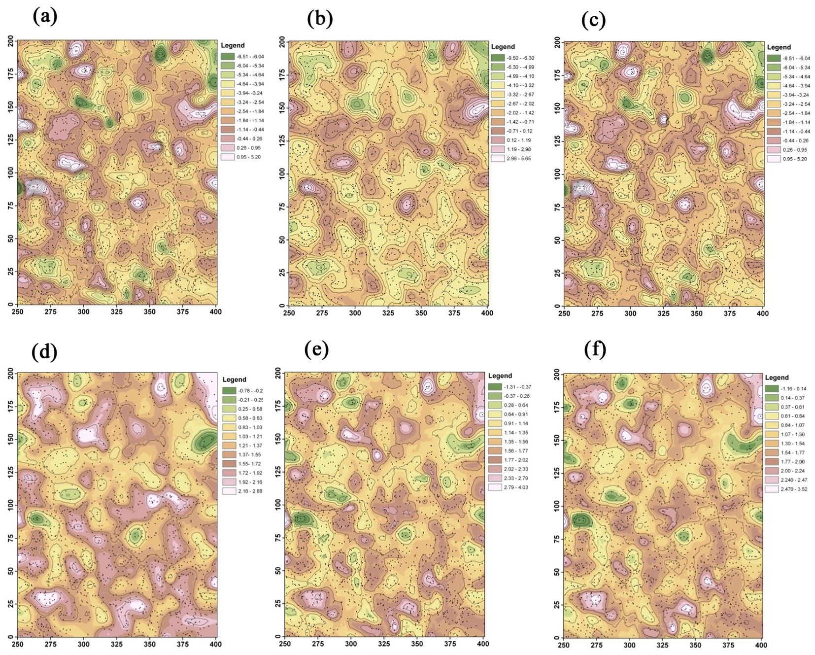
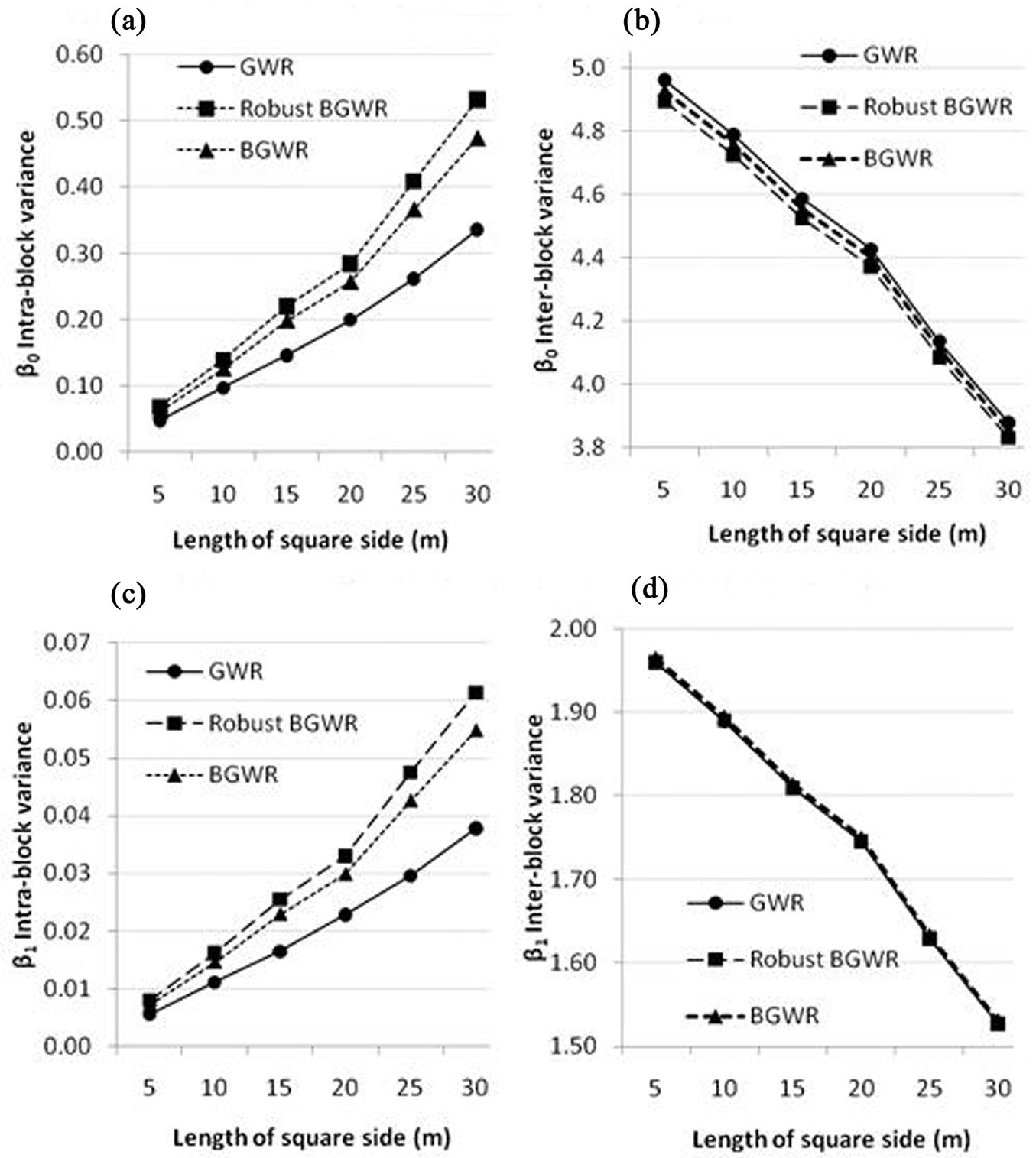
Fig. 5 shows the intra-block Vintra (eqn. 14) and inter-block Vinter (eqn. 15) variances of the two coefficients (β0 and β1) from the three modeling methods. In general, Vinter indicates the regional spatial variability, while Vintra quantifies the local spatial variability. When the block size increases, Vintra increases and Vinter decreases. Fig. 5 indicates the three modeling methods yielded similar inter-block variances (regional spatial variability) for the two coefficients across different block sizes. In contrast, rBGWR produces the largest localized spatial variability for both coefficients (i.e., the largest Vintra), followed by BGWR, while GWR had the smallest Vintra for both coefficients, implying that the two regression coefficients were more similar within blocks (probably appeared as “hot” or “cold” spots in Fig. 4).
Fig. 5 - Intra-block variances (Vintra) and inter-block variances (Vinter) of local regression coefficients from the three modeling methods. (a) Intra-block - β0; (b) Inter-block - β0; (c) Intra-block - β1; (d) Inter-block - β1.
Simulated data
Model fitting
Tab. 5 shows the model fitting statistics and the range of the heteroscedastic variance V(si) by BGWR (with r = 4, 5 and 6, and δ2 = 50% only) and rBGWR (with r = 4, 5 and 6). It seems that for BGWR increasing the prior of r increased the model deviance D(β), but the model complexity (pD) decreased. In the case of rBGWR, as the prior mean for r increased, the model deviance increased, but the model complexity remained flat. However, the DIC indicated both BGWR and rBGWR fitted the data better with smaller prior of r. Because the simulated data had outliers, the choice of smaller mean prior on r allowed for larger variation in V(si) and consequently improved the model fit ([19], [26]).
Tab. 5 - Model fitting statistics for BGWR and rBGWR to the simulated data. BGWR models were fitted with scale factor = 50%.
| Method | Model | Prior Mean of r |
DIC | D(β) |
pD | V(si) | ||
|---|---|---|---|---|---|---|---|---|
| Min | Max | STD | ||||||
| BGWR | 1 | 4 | 1567.24 | 632.04 | 935.21 | 0.9949 | 1.0212 | 0.0022 |
| 2 | 5 | 1587.61 | 699.24 | 888.36 | 0.9957 | 1.0204 | 0.0019 | |
| 3 | 6 | 1651.40 | 750.07 | 875.07 | 0.9964 | 1.0196 | 0.0017 | |
| rBGWR | 4 | 4 | 1550.99 | 746.42 | 804.57 | 1.0400 | 30.8000 | 0.8891 |
| 5 | 5 | 1568.63 | 764.23 | 804.40 | 1.0300 | 14.7800 | 0.4192 | |
| 6 | 6 | 1583.89 | 776.21 | 807.68 | 1.0000 | 8.3100 | 0.2276 | |
Similar to the results obtained for the observed data, the posterior mean of V(si) was sensitive to the priors of r for rBGWR, but not so sensitive for BGWR (Tab. 5). Based on the model fitting statistics, the BGWR and rBGWR models with r = 4 were chosen to compare with GWR. As mentioned earlier, the DIC value was not calculated for GWR. However, the coefficient of determination of the GWR model was 0.75 for fitting the simulated data. It was not surprising that the coefficient of determinations of GWR were very similar for the observed and simulated data since the two datasets had similar descriptive statistics (see Tab. 1 and Tab. 2) and features (e.g., cluster pattern, large variation in dbh). The coefficient of determination of GWR for simulated data (0.75) was slightly lower than that for observed data (0.78) because simulated data have more outliers than observed data.
A summary of descriptive statistics on the local regression coefficients estimated by the three modeling methods are given in Tab. 6, along with the summary for the simulated “true or known” coefficients for each location. It appears that the posterior mean and median of the slope coefficient (β1) estimated by the three modeling methods are very similar from each other, as well as similar to the “known β1”. On the other hand, the posterior mean and median of the intercept coefficient (β0) were larger than the “known β0”. In addition, the estimated two local coefficients by the three modeling methods had much larger standard deviations and ranges than the “known” simulated coefficients (Tab. 6). The reasons were that the simulated “true or known” coefficients were individually generated using the bivariate Gaussian copulas with a given measure of association between the two coefficients β0 and β1, while the local coefficients estimated by the three modeling methods were based on the response variable ln(crown) and explanatory variable ln(dbh) of the neighboring trees for each subject location. Hence, larger variances in the estimated local coefficients by the three modeling methods were not surprising.
Tab. 6 - Summary of local regression coefficients from GWR, BGWR and rBGWR methods for the simulated data. Q1, Q3, P2.5 and P97.5 are lower quartile, upper quartile, 2.5th percentile, and 97.5th percentile, respectively. (SD): standard deviation.
| Coefficient | Method | n | Mean | Median | Q1 | Q3 | P2.5 | P97.5 | Min | Max | SD |
|---|---|---|---|---|---|---|---|---|---|---|---|
| Intercept β0 | Simulated | 1230 | 0.201 | 0.198 | 0.096 | 0.312 | -0.08 | 0.478 | -0.260 | 0.58 | 0.143 |
| GWR | 1230 | 0.231 | 0.265 | -0.124 | 0.685 | -1.526 | 1.683 | -7.656 | 4.801 | 0.917 | |
| BGWR | 1230 | 0.300 | 0.302 | -0.131 | 0.788 | -1.436 | 2.002 | -7.702 | 3.303 | 0.847 | |
| rBGWR | 1230 | 0.298 | 0.302 | -0.16 | 0.812 | -1.456 | 2.035 | -7.805 | 3.462 | 0.87 | |
| Slope β1 | Simulated | 1230 | 0.811 | 0.800 | 0.696 | 0.903 | 0.610 | 1.079 | 0.600 | 2.248 | 0.154 |
| GWR | 1230 | 0.797 | 0.781 | 0.622 | 0.939 | 0.278 | 1.418 | -0.448 | 3.613 | 0.334 | |
| BGWR | 1230 | 0.766 | 0.765 | 0.583 | 0.941 | 0.158 | 1.401 | -0.349 | 3.272 | 0.313 | |
| rBGWR | 1230 | 0.766 | 0.764 | 0.576 | 0.948 | 0.143 | 1.423 | -0.430 | 3.304 | 0.322 |
Accuracy and bias in estimates of local coefficients
The 95% credible limits of each model coefficient for both BGWR and rBGWR were used to assess the accuracy of estimates of the local model coefficients. If the 95% credible limit of a coefficient for a particular location included the “known” simulated coefficient, the coefficient estimated by that method for that location was declared to be unbiased. The results indicated that, out of 1230 comparisons, 853 (69.3%) of β0 and 903 (73.4%) of β1 by BGWR, and 864 (70.2%) of β0 and 912 (74.1%) of β1 by rBGWR, respectively, were unbiased. When the two coefficients were compared simultaneously, the rBGWR method (839 or 68.2%) was slightly better than the BGWR method (826 or 67.2%).
Sensitivity to outliers
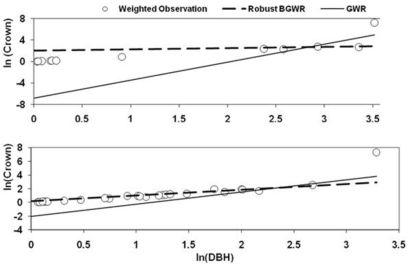
To assess the sensitivity of GWR and rBGWR to outliers in the data, two outliers (Tree ID 141 and 541) were selected to compare the local coefficients by the two methods. Fig. 6 shows the scatterplot of ln(crown) and ln(dbh), including all observations within the given bandwidth. The regression lines of GWR and rBGWR were generated using coefficients of these methods. It was clear that the rBGWR coefficients were indeed “robust” to the outlier, while the GWR coefficients were strongly affected by the outlier that pulled the regression line of GWR up and resulted in smaller slope coefficient and larger and negative intercept coefficient. This result was expected as GWR uses weighted least square method with constant variance to estimate the local coefficients. In contrast, the rBGWR method assumes heterogeneous variances and gave larger variance to the outlier. In addition, rBGWR used W(si)/V(si) as the spatial weight for estimating the coefficients. For example, rBGWR estimates V(si) were 6.87 for Tree ID 141 and 7.68 for Tree ID 541, respectively. Due to the lager variances, the spatial weights of the outliers were diminished heavily to 0.145 for Tree ID 141 and 0.13 for Tree ID 541, respectively.
Fig. 6 - The outlier and neighboring observations within the bandwidth. The two regression lines of GWR and rBGWR were generated using the estimated slope and intercept coefficients. The response variable (crown area) and explanatory variable (dbh) are weighted by proximity to outlier observations and expressed in logarithmic scale.
Weak data scenario
Tab. 7 showed the simulated coefficients and the GWR local coefficients, and the 95% credible limits of the two coefficients by BGWR and rBGWR for eight selected weak data observations. BGWR and rBGWR produced unbiased coefficients (i.e., the simulated coefficients were within the 95% credible limits of estimated coefficients) for five (5) observations among the eight (8) weak observations compared. The rBGWR method produced the smallest prediction error for these weak observations, followed by BGWR, and GWR (results not shown), implying that rBGWR and BGWR are more accurate in estimating the local coefficients and predicting the response variable than GWR when the weak data problems exists.
Tab. 7 - Simulated and geographically weighted regression (GWR) estimated coefficients, and Bayesian geographically weighted regression (BGWR) and robust BGWR (rBGWR) estimated 95% credible limits of coefficients for weak observations in simulated data. (‡): indicates the 95% of credible limits of BGWR and rBGWR coefficients that do not contain simulated coefficients.
| Coefficients | Tree ID | Location | Simulated | GWR | BGWR | rBGWR | |||
|---|---|---|---|---|---|---|---|---|---|
| Easting | Northing | 95% Credible limits | 95% Credible limits | ||||||
| Intercept | 133 | 75.1 | 15.5 | -0.023 | -0.392 | -0.661 ‡ | -0.094 ‡ | -0.553 ‡ | -0.179 ‡ |
| 174 | 37.5 | 21.9 | 0.014 | 1.556 | -0.544 | 2.607 | -0.438 | 2.583 | |
| 265 | 59.9 | 31.8 | 0.080 | -0.708 | -6.598 | 5.564 | -4.230 | 3.138 | |
| 620 | 32.7 | 74.7 | 0.020 | -0.880 | -2.913 | 1.048 | -2.623 | 0.619 | |
| 649 | 85.2 | 76.6 | 0.340 | -0.040 | -0.189 ‡ | 0.132 ‡ | -0.190 ‡ | 0.130 ‡ | |
| 924 | 142.6 | 23.1 | 0.135 | -0.120 | -1.103 | 0.871 | -0.918 | 0.757 | |
| 925 | 137.5 | 21.9 | 0.399 | -1.681 | -4.007 ‡ | -0.286 ‡ | -4.034 ‡ | -0.484 ‡ | |
| 1132 | 132.7 | 74.7 | 0.119 | 0.130 | -0.802 | 0.791 | -0.738 | 0.679 | |
| Slope | 133 | 75.1 | 15.5 | 0.925 | 1.045 | 0.945 ‡ | 1.136 ‡ | 0.974 ‡ | 1.096 ‡ |
| 174 | 37.5 | 21.9 | 0.971 | 0.341 | -0.082 | 1.191 | -0.070 | 1.153 | |
| 265 | 59.9 | 31.8 | 0.951 | 1.235 | -1.083 | 3.409 | -0.174 | 2.543 | |
| 620 | 32.7 | 74.7 | 1.034 | 1.301 | 0.653 | 1.995 | 0.827 | 1.903 | |
| 649 | 85.2 | 76.6 | 0.700 | 0.864 | 0.793 ‡ | 0.929 ‡ | 0.792 ‡ | 0.930 ‡ | |
| 924 | 142.6 | 23.1 | 0.853 | 0.941 | 0.584 | 1.313 | 0.620 | 1.248 | |
| 925 | 137.5 | 21.9 | 0.649 | 1.496 | 0.931 ‡ | 2.433 ‡ | 1.008 ‡ | 2.444 ‡ | |
| 1132 | 132.7 | 74.7 | 0.837 | 0.824 | 0.601 | 1.140 | 0.650 | 1.119 | |
Discussion
In this study, we established a relationship between tree crown and dbh for observed and simulated data using GWR, BGWR and rBGWR, and demonstrated the advantages of Bayesian approach to improve the model fitting and performance of GWR. Firstly, BGWR and rBGWR not only provided better estimation of local regression coefficients, but also correct estimation of the variances of the coefficients because Bayesian procedures (e.g., Gibbs sampler) are not affected by the lack of independence in the sample data. Thus, correct statistical inference and creditable limits (or confidence intervals) can be computed and used for statistical testing and model interpretation. The average prediction errors yielded by BGWR and rBGWR were only about 50% of that produced by GWR across all DBH classes. Secondly, the estimates of local coefficients by rBGWR were not affected by potential outliers, while these estimates by GWR were “contaminated” by the outliers (e.g., producing smaller slope and larger and negative intercept). It is not uncommon that forestry and/or ecological data have potential outliers or unusual observations. If the coefficient estimates of a model are sensitive to the outliers, it could have serious implication for interpreting the meaning of the coefficients as well as the regression relationships between variables. BGWR and rBGWR can automatically detect and down-weight the outliers’ influence in the parameter estimation processes. Furthermore, when the spatial pattern of trees or plants is clustered, there are good chances that the number of trees could be sparse in some locations, resulting in very small number of effective observations that can be used to estimate the model parameters (i.e., the weak data problem). BGWR and rBGWR are able to produce unbiased estimation on model parameters and prediction by incorporating prior information, such as expert opinion or existing knowledge, to impose restrictions on the spatial nature of parameter variation ([27]). According to our results, rBGWR produced the smallest prediction error in weak data scenario, followed by BGWR and GWR. When large spatial data sets are involved in data analysis and modeling, heterogeneous variance may be a serious issue for model parameter estimation. BGWR combines the distance-based spatial weight matrix, non-constant variance in model error term and any prior information into a parameter smoothing specification as a unified parameter estimation approach to overcome the limitations of GWR ([27], [50]).
However, the BGWR methods need to be used with caution. Given their nature, the local coefficients estimated by the BGWR methods may not be used to make prediction outside the study area. Attention should be given to assess potential model misspecification, because the spatial heterogeneities of the relationships between variables might have been produced as a result of model misspecification ([8], [13]). The assessment of residuals may be useful for identifying model misspecification ([52]).
One of the challenges on modeling spatial effects (i.e., spatial autocorrelation and heterogeneity) is to identify an appropriate spatial scale ([12]). Changes in the bandwidth or number of neighbors will result in change of support ([20]), and consequently will produce different model fitting and parameter estimates ([22]). Larger bandwidth will delineate a broader region as neighborhood and will smooth the spatial heterogeneity rather too much, while smaller bandwidth will define a limited area as neighborhood and will produce too “spiky” spatial heterogeneity ([51], [1]). For the choice of scale (in this study bandwidth and number of neighbors), Wagner & Fortin ([47]) suggested that the scale of analysis needs to be determined in an ecologically meaningful and methodologically sound way.
Another challenge to the BGWR methods is related to the convergence of parameters. In this study, longer MCMC chains were used to sample the posterior distributions of local coefficients. While sampling posterior of coefficients for nine BGWR models (with a combination of the priors on variance and scale factor) and for three rBGWR models (with three priors on variance), the slope and intercept coefficients estimated by these models converged at the desired level of precision (quartile = 0.025, precision = 0.005 and probability = 0.95) for most of the observations within the 4.000 runs after the few thousands initial burn-in and storing one sample out of 10 samples. However, for a few observations, those that fall at the edge of the study area required almost 15.000 iterations (at the maximum for the BGWR method with prior on scale factor at the smallest level) to converge. The assessment of histogram of coefficients and its movement across iterations also suggested the desirability of longer runs for the latter observations. One of the reasons for the convergence problem may be the correlation between the parameters within the parameter set ([7]). However, the autocorrelation among the posterior sample of coefficients can be reduced by thinning, e.g., keeping one coefficient out of 10 sampled coefficients. In contrast, the BGWR method posterior sample of coefficients with large (the largest level) prior on scale factor converged more quickly than those with small (the smallest level) prior on scale factor. In the case of the rBGWR method, which samples all the posterior samples of coefficients for an observation before moving to the next observation, this method took less time to run. Besides this, the computation time was directly related to the precision level required for parameter convergence; e.g., for smaller precision (quartile = 0.025, precision = 0.01 and probability = 0.95), the estimates of coefficients by rBGWR and BGWR converged within a few thousands of iterations after sufficient burn-in.
Despite these limitations, BGWR methods have been recommended as an effective tool for investigating spatial heterogeneity of covariate effects across a study area. Future studies on developing an optimization method as a function of both bandwidth and covariates are recommended. The current approach of bandwidth optimization (e.g., the CV method) optimizes only bandwidth for a given set of covariates. A better method that optimizes a combination of covariates (similar to forward or backward selection in regression) and bandwidth simultaneously is more desirable. In addition, a window-driven software for parameter estimation by the BGWR methods would certainly be an asset for wider adaptations of these Bayesian methods.
Conclusion
The relationship between tree crown area and diameter at breast height was modeled using GWR, BGWR, and rBGWR models. Both observed and simulated tree data were used to compare model fitting and performance. For the observed Ontario softwood stand, BGWR and rBGWR produced more accurate parameter estimates and better model prediction than GWR. Further, rBGWR produced the largest localized spatial variability for both coefficients, followed by BGWR, while GWR had the smallest localized spatial variability for both coefficients. Thus, the contour maps of local regression coefficients show more “hot” or “cold” spots of the two coefficients estimated by GWR than those obtained by BGWR and rBGWR.
For the simulated data, the percentage of the unbiased parameter estimation for the two local coefficients by rBGWR was slightly higher than those by BGWR. However, the credible limits cannot be computed for GWR due to the lack of an accurate expression of the variance of the model coefficients in GWR. Further, the coefficients estimates using the rBGWR method were not affected by outliers, while these estimates by GWR were “contaminated” by the outliers, resulting in erroneous parameter estimates. Similarly, for the weak data, the majority of the coefficients estimated by the rBGWR and BGWR methods were not different from the simulated “known” coefficients. Therefore, BGWR and rBGWR are better alternatives to overcome the limitations of GWR and are more powerful than GWR to detect the spatial areas with non-constant variance or spatial outliers.
Acknowledgements
This work was supported by the National Natural Science Foundation of China, proj. no. 31400491: “Three dimensional individual tree crown delineation based on multiple remotely sensed data sources and tree competition mechanism”, and by the Fundamental Research Funds for the Central Universities, proj. no. 2572017CA02.
References
Gscholar
Gscholar
Gscholar
Gscholar
Gscholar
Gscholar
Gscholar
Gscholar
Gscholar
Gscholar
Gscholar
Gscholar
Gscholar
Gscholar
CrossRef | Gscholar
Gscholar
Gscholar
Gscholar
Authors’ Info
Authors’ Affiliation
Lianjun Zhang
Department of Forest and Natural Resources Management, State University of New York College of Environmental Science and Forestry, One Forestry Drive, Syracuse, NY 13210 (USA)
School of Forestry, Northeast Forestry University, Harbin (China)
Corresponding author
Paper Info
Citation
Subedi N, Zhang L, Zhen Z (2018). Bayesian geographically weighted regression and its application for local modeling of relationships between tree variables. iForest 11: 542-552. - doi: 10.3832/ifor2574-011
Academic Editor
Luca Salvati
Paper history
Received: Jul 30, 2017
Accepted: Jun 11, 2018
First online: Sep 01, 2018
Publication Date: Oct 31, 2018
Publication Time: 2.73 months
Copyright Information
© SISEF - The Italian Society of Silviculture and Forest Ecology 2018
Open Access
This article is distributed under the terms of the Creative Commons Attribution-Non Commercial 4.0 International (https://creativecommons.org/licenses/by-nc/4.0/), which permits unrestricted use, distribution, and reproduction in any medium, provided you give appropriate credit to the original author(s) and the source, provide a link to the Creative Commons license, and indicate if changes were made.

Web Metrics
Breakdown by View Type
Article Usage
Total Article Views: 50664
(from publication date up to now)
Breakdown by View Type
HTML Page Views: 41279
Abstract Page Views: 3310
PDF Downloads: 4954
Citation/Reference Downloads: 10
XML Downloads: 1111
Web Metrics
Days since publication: 2877
Overall contacts: 50664
Avg. contacts per week: 123.27
Article Citations
Article citations are based on data periodically collected from the Clarivate Web of Science web site
(last update: Mar 2025)
Total number of cites (since 2018): 9
Average cites per year: 1.13
Publication Metrics
by Dimensions ©
Articles citing this article
List of the papers citing this article based on CrossRef Cited-by.
Related Contents
iForest Similar Articles
Research Articles
Distribution factors of the epiphytic lichen Lobaria pulmonaria (L.) Hoffm. at local and regional spatial scales in the Caucasus: combining species distribution modelling and ecological niche theory
vol. 17, pp. 120-131 (online: 30 April 2024)
Research Articles
A geographically weighted deep neural network model for research on the spatial distribution of the down dead wood volume in Liangshui National Nature Reserve (China)
vol. 14, pp. 353-361 (online: 27 July 2021)
Research Articles
Spatial distribution of aboveground biomass stock in tropical dry forest in Brazil
vol. 16, pp. 116-126 (online: 17 April 2023)
Research Articles
Spatial heterogeneity of soil respiration in a seasonal rainforest with complex terrain
vol. 6, pp. 65-72 (online: 07 February 2013)
Research Articles
Comparison of parametric and nonparametric methods for modeling height-diameter relationships
vol. 10, pp. 1-8 (online: 19 October 2016)
Research Articles
Yield of forests in Ankara Regional Directory of Forestry in Turkey: comparison of regression and artificial neural network models based on statistical and biological behaviors
vol. 16, pp. 30-37 (online: 22 January 2023)
Research Articles
Estimating biomass of mixed and uneven-aged forests using spectral data and a hybrid model combining regression trees and linear models
vol. 9, pp. 226-234 (online: 21 September 2015)
Research Articles
Modeling compatible taper and stem volume of pure Scots pine stands in Northeastern Turkey
vol. 16, pp. 38-46 (online: 22 January 2023)
Research Articles
Geographic determinants of spatial patterns of Quercus robur forest stands in Latvia: biophysical conditions and past management
vol. 12, pp. 349-356 (online: 05 July 2019)
Research Articles
Spatial diversity of forest regeneration after catastrophic wind in northeastern Poland
vol. 9, pp. 414-421 (online: 29 January 2016)
iForest Database Search
Search By Author
Search By Keyword
Google Scholar Search
Citing Articles
Search By Author
Search By Keywords
PubMed Search
Search By Author
Search By Keyword


