Modeling compatible taper and stem volume of pure Scots pine stands in Northeastern Turkey
iForest - Biogeosciences and Forestry, Volume 16, Issue 1, Pages 38-46 (2023)
doi: https://doi.org/10.3832/ifor4099-015
Published: Jan 22, 2023 - Copyright © 2023 SISEF
Research Articles
Abstract
Compatible taper and volume equations for pure and natural Scots pine stands in the northeastern part of Turkey (Ardahan Province) were developed using a nonlinear mixed-effects modeling approach. Experimental data were obtained from 137 felled sample trees in different diameter and height classes. The most successful model ([21]) explained 98.3% of the variance in stem diameter estimation and the RMSE, ME, MAE, AIC and BIC value obtained using this model were 1.955 cm, 0.043 cm, 1.300 cm, 9783.8 and 9812.6, respectively. Considering the criterion values of AIC, BIC and -2LnL, the model with random-effects in two parameters (b1 and b3) was the most successful for Scots pine. While the mixed model including random parameters did not completely solved the problem of the autocorrelation of errors in this study, the use of the autoregressive error structure AR(1) eliminated the autocorrelation in the residuals. In addition, the best estimation results among 20 different calibration options were obtained using the option of measuring two tree diameters at d1.30 and d5.30 with validation data. The most successful model explained 99.18% of the total variance in stem volume estimation in Scots pine.
Keywords
Nonlinear Mixed-effects Model, Segmented Polynomial Taper Models, Calibration, Random Parameters, Autocorrelation, Stem Volume
Introduction
Scots pine (Pinus sylvestris L.) is one of the most important commercial forest tree species in Turkey due to its wide spatial distribution, economic value, growth and wood structure. According to the forest inventory data of the Turkish General Directorate of Forestry in 2015, Scots pine covers nearly 1.518.929 ha (6.80%) of the total forest area of the country ([15]). Almost 192.233 ha (12.7%) of Scots pine forests are located in the Erzurum Regional Directorate of Forestry, of which 25.159 ha (13.1%) are located in Ardahan State Forest Enterprise (SFE), the case study area.
While the volume of trees can be practically calculated using various tree volume equations, the volume or proportions of derived wood assortments such as mine poles, industrial wood, pulp and paper, and firewood cannot be so easily determined. For this reason, taper models that provide detailed estimates of both tree volume and wood assortments are needed ([11], [6], [17], [18]). Indeed, the stem diameter of a tree gradually decreases from the base to the top, and the rate of decrease in diameter along the stem is called the stem taper. The rate at which stem diameter decreases upwards depends on tree species, age, spatial conditions, tree genetics, silvicultural practices, site conditions and climatic characteristics ([37]). Equations for stem diameter and volume are important components of forest inventory, growth and yield modeling, forest management planning, and product simulation systems ([38], [41]). To describe stem taper throughout the bole with different geometric solids, compatible taper models with a set of sub-models have long been used ([13], [51], [35], [41]). According to Kozak ([25]), these taper models provide estimates of: (i) diameter inside or outside bark at any height of the stem; (ii) height of any stem diameter; (iii) total stem volume; (iv) merchantable volume; (v) the volume of wood assortment; (vi) individual volume for logs between any two heights; and (vii) individual volumes for logs between any two diameters on the stem ([4], [33], [44]).
Since the 1900s, many stem profile models in different forms have been developed. According to Diéguez-Aranda et al. ([11]), these stem profile models have been classified as simple stem profile models ([10]), variable-form stem profile models ([5], [29], [25]), and segmented stem profile models ([32], [36], [13], [21]). The success of these models varies depending on the tree species, data set and model structure ([40], [33]). The models of the first group describe tree taper using a simple mathematical function which can be either trigonometric, polynomial, or a power function. In the models of the second group, a single continuous function with an exponent that changes from the base to the top describes various intermediate shapes such as neiloids, cones and paraboloids. The models in the last group, the segmented polynomial taper models, are compatible taper models and can estimate the entire stem profile in the most realistic way, since they split the tree stem into appropriate sections and calculate each section separately ([24]). An important advantage of these stem profile models over other models is that stem profile models can be easily converted into equations for volume calculations ([13]). The compatible segmented taper models for commercially available tree species are very useful and flexible tools for both forest research studies and forest inventory ([45], [1]).
Diameters measured at different heights on a single tree are used as an important data source for developing stem profile models. Consequently, sequential measurements along the tree stem are related with each other ([14]). According to Leites & Robinson ([30]), “in a hierarchical data structure where each tree has its own stem development, there may be interdependence of the data, which is called a «series-correlation» or «autocorrelation» problem” ([7], [16]). Such serial correlation between sample data leads to systematic error in the estimation of confidence intervals of parameter estimates of stem diameter and stem volume equations, and thus negatively affects the reliability the model results ([43], [27]). Therefore, for hierarchical data structures where the assumption of data independence cannot be achieved and there is a problem of serial correlation between data, the use of the nonlinear mixed-effects (NLME) modeling approach is recommended to model the variance-covariance matrix structure ([23]). If the mixed model that includes random parameters does not completely eliminate autocorrelation of the errors, the autoregressive error structure AR(1) can remove the autocorrelation in the residuals ([35], [20]).
Stem diameters at different heights and stem volume predictions of commercial trees such as Scots pine are critical for developing thorough forest management plans. This study focuses on developing compatible taper and volume models, which allow comprehensive volume and diameter estimations for pure and natural Scots pine stands distributed in the Ardahan SFE of Erzurum Regional Directorate of Forestry, using the nonlinear mixed-effect modeling approach.
Materials and methods
Materials
Pure Scots pine stands are naturally distributed in the Ardahan province, Northeastern Turkey (40° 45′ 24″ - 41° 36′ 13″ N, 42° 25′ 43″ - 43° 29′ 17″ E), where the monthly average temperature ranges from -11.1 to +16.4 °C (annual average of 3.9°C), the lowest temperature is between -39.8 °C and -2.2 °C, and the highest temperature reaches 35 °C. The average total annual precipitation is 573.9 mm and the average annual relative humidity varies between 65% and 71% ([2]). Ardahan has a continental climate with long winters (seven months), very short spring and fall months, cool summers and springs.
The area of the Ardahan State Forest Enterprise is approximately 547,671 ha, of which 30,757.4 ha (5.6%) are covered by forests and 516,913.6 ha (94.4%) are bare lands. Of the forested area, 24,343.3 ha (79%) are productive forests, while 6,414.1 ha (21%) are unproductive or degraded forests.
The case study area covers 24.106 ha of pure Scots pine forests in the Ardahan region, which are managed under five different management units; 3819 ha are assigned to the Ardahan forest management unit, 4525 ha are assigned to the Köroglu forest management unit, 1582 ha are assigned to the Posof forest management unit, 7865 ha are assigned to the Ugurlu forest management unit and 6314 ha are assigned to the Yalnizçam forest management unit ([2]). The spatial distribution of pure Scots pine stands in the case study area is shown in Fig. S1 (Supplementary material).
Data from 137 sample trees felled in pure and natural Scots pine stands in Ardahan SFE, Erzurum Regional Directorate of Forestry, were used as source material for this case study. In the selection of the sample trees, due care was taken to distribute them as equally and evenly as possible in different diameter and height classes and to best reflect the variability in volume development.
The sample trees were cut from the base diameter of the stem (0.3 m above the ground), and then the bottom diameter of he log (0.3 m), the diameter at breast height (1.3 m), and other diameters at 1 meter regular intervals (2.3 m, 3.3 m, 4.3 m etc.) were measured. All measures were taken using calipers with an accuracy of ± 1.0 mm. In addition, the heights of the trees were measured with a steel tape measure to an accuracy of ± 1.0 cm. The diameters of non-circular sections on the stem were measured in two directions perpendicular to the stem section and their average was calculated.
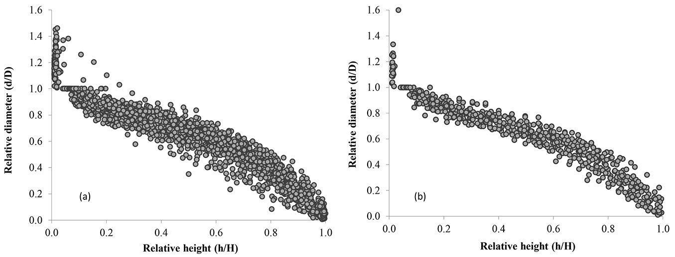
A total of 2939 diameter measurements were taken from the 137 sample tree stems felled within the scope of this study. The data used in the study were randomly divided into two groups: (i) the data used to estimate the parameters of the stem profile models (Group I data: approximately 80% of the total data - 2340 stem diameter records from 110 trees); and (ii) the data used to validate the suitability of these models for the stand (Group II data: approximately 20% of the total data - 599 record from 27 trees). Fig. 1shows the distribution of relative diameters by relative height values for both the training and the validation data sets for Scots pine trees. Statistical information and some tree characteristics of 137 sample trees felled in the Ardahan forests are presented in Tab. 1.
Fig. 1 - Plots of the relative height versus relative diameter outside bark for (a) the fitting data points, and (b) the validation data points.
Tab. 1 - Descriptive statistics for the fitting and the validation data points. (D): diameter at breast height (cm); (H): total height (m); (t): tree age (year); (v): tree volume (m3); (d): diameter outside bark at specific height; (h): height at specific diameter; (n): number of observations; (SD): standard deviation.
| Data type |
Variable | n | Minimum | Mean | Maximum | SD |
|---|---|---|---|---|---|---|
| Fitting data | D (cm) | 110 | 6.0 | 35.3 | 74.5 | 16.2 |
| H (m) | 110 | 6.6 | 21.0 | 32.0 | 5.5 | |
| t (yil) | 110 | 19.0 | 99.2 | 181.0 | 37.3 | |
| v (m3) | 110 | 0.008 | 1.317 | 5.920 | 1.315 | |
| d (cm) | 2340 | 0.2 | 24.0 | 86.0 | 15.2 | |
| h (m) | 2340 | 0.3 | 11.1 | 31.3 | 7.1 | |
| Validation data | D (cm) | 27 | 7.5 | 36.5 | 66.0 | 15.0 |
| H (m) | 27 | 8.7 | 21.9 | 30.7 | 4.6 | |
| t (yil) | 27 | 17.0 | 103.3 | 171.0 | 32.2 | |
| v (m3) | 27 | 0.022 | 1.337 | 4.465 | 1.123 | |
| d (cm) | 599 | 0.5 | 24.2 | 72.0 | 14.2 | |
| h (m) | 599 | 0.3 | 11.3 | 30.3 | 7.1 |
Methods
Segmented polynomial taper models
We used four segmented polynomial stem profile models which have been employed in other similar studies: Model 1 by Jiang et al. ([21]), Model 2 by Max & Burkhart ([32]), Model 3 by Parresol et al. ([36]), and Model 4 by Fang et al. ([13]). All models used in this study are compatible and segmented polynomial stem profile models. The equations for various compatible taper and stem volume models used are described in Tab. S1 (Supplementary materials). Jiang et al. ([21]) used a reduced form of Clark et al. ([9]) taper model.
The NLIN procedure of the software package SAS/STAT® v. 9.3 was used to estimate the parameters of the four stem taper and volume models ([42]). The adjusted coefficient of determination (Radj2), Root-Mean-Square Error (RMSE), Mean Error (ME), Mean Absolute Error (MAE), Akaike’s Information Criterion (AIC) and Schwarz’s Bayesian Information Criterion (BIC) were used to evaluate the performance of the stem taper models (eqn. 1 to eqn. 6). Actually, it is desirable that the adjusted coefficient of determination (Radj2) is close to 1 and the other criteria are lower ([8], [46], [22]). The model evaluation criteria were given in the following equations (eqn. 1 to eqn. 6):
where n is the number of observations; p is the number of coefficients in the model; yi, {hat}yi and {bar}y are the observed, predicted and average diameters outside bark, respectively; k is the number of parameters in the model; L is the maximum likelihood value (ML).
After determining the best-fit of the above four segmented stem profile models, the mixed-effects modeling approach was used to estimate the best-fit stem diameter model.
Nonlinear mixed-effects modeling approach
Different diameter values measured along each log were used to develop the taper models. Diameters taken from the same log are interdependent (serial correlation or “autocorrelation”), thus one of the basic assumptions of regression analysis is neglected ([48]). According to Ye ([50]), the violation of this assumption can lead to the estimation of parameter confidence intervals with a systematic error, which negatively affects the reliability of the model and results in erroneous estimates. In the development of regression models, the nonlinear mixed-effects model (NLME) approach, which specifically allows the modeling of the variance-covariance matrix structure, is recommended instead of using nonlinear regression analysis and parameter estimation procedures based on different numerical analysis methods ([23]).
In the mixed-effects model, parameters are divided into two groups: fixed and random effects. The fixed effect parameter expresses the general relationships that apply to the entire population. The random effect parameter describes the variability between different sampling units (sample trees). The structure of the nonlinear mixed-effects model is presented below in the form of a matrix (eqn. 7, eqn. 8):
where Yij is the value of the dependent variable for the j-th measurement of the i-th sampling tree; f is a nonlinear function; Φi are the parameter values of the model; Xij is the value of the independent variable for the j-th measurement of the i-th sampling tree; εij are the model errors [=N(0,R)]; β is the fixed-effects parameter vector computed for the entire population; bi = N(0,D) is a vector of random parameters (indicating the difference between sample trees) having a multivariate normal distribution with mean bi of 0 and variance-covariance matrix D; Aij and Bij are the fixed-effect and random-effect parameters, respectively. The component D is a positive definite variance-covariance matrix expressing the variability between the sample trees (between trees variability); the component R represents the variance-covariance matrix describing the variability (within-trees variability) between the measured data in the sample trees ([8], [47], [1], [17]).
The parameters of Jiang et al. ([21]) stem taper model were estimated in this study via AR (1) autoregressive modeling to remove the autocorrelation between the data collected as time series, especially the stem analysis data. The AR (1) autoregressive modeling has been used in many studies and is recommended especially when nonlinear mixed-effects modeling does not completely remove the autocorrelation of errors ([35], [24], [20]).
The variance components and constant parameters of the best-fit stem profile model were estimated using the PROC NLMIXED procedure in the SAS/ETS® v. 9.3 statistical package ([42]). This method was used to test different random parameter combinations to create the best stem profile model. Root-Mean-Square Error (RMSE), Akaike’s Information Criterion (AIC), Schwarz’s Bayesian Information Criterion (BIC) and twice the negative log-likelihood (-2LnL) criteria were used to determine the best-fitting parameter combination for the random effect.
Calibration responses
Another important issue to be evaluated and solved in mixed-effects modeling is the identification of the “calibration responses” of the model. Calibrated models offer the possibility of more accurate, consistent, and reliable estimates ([8], [47], [49], [7]). In mixed-effects models, random parameters are calculated using newly obtained observed values from the sample areas by adding this random parameter to the fixed-effect parameter values valid for the entire population and calculating the valid parameter values for the sample area under study. The Best Linear Unbiased Predictor (BLUP) method is used to calibrate mixed models in forestry.
BLUP requires the measurement of a certain number of new data in a site or sample area to be calibrated, especially when estimating the random-effect parameter ([17]). In particular, the determination of the trees (thickest, thinnest or near-median diameter trees) to be measured in the sample areas is referred to as the “calibration response” of the mixed-effects models. For this purpose, random parameters are calculated using trees with different characteristics in the same sample areas, and the error values of the estimates obtained in the next step are analyzed. The random effects parameter was estimated using the following equation ([47], [49] - eqn. 9):
where D and R are the variance-covariance matrices previously defined; Zi is the design matrix for the random-effects parameters; Zi′ represents the inverse of the Zi matrix. In addition, the component Yi - Aijβ in the above equation is calculated by subtracting the estimate to be made using only fixed-effect parameters in the mixed model from the observed value.
In determining the calibration response of the mixed effects models with validation data, the Sum of Squared Errors (SSE, eqn. 10), Mean Squared Error (MSE, eqn. 11) and Root-Mean-Square Error (RMSE, eqn. 2) were calculated ([8]):
Results and discussions
Model selection for stem taper
Goodness-of-fit statistics of the stem profile models successfully fitted to the data set are given in Tab. 2. Model 1 ([21]) accounted for 98.34% of the total variance in stem diameter estimates, Model 4 ([13]) explained 97.82%, while Model 2 ([32]) and Model 3 ([36]) explained 97.74% and 97.26% of the total variance, respectively. The coefficients of determination of the stem profile models (Radj2) ranged from 0.9726 to 0.9834, the standard errors (RMSE) between 1.955 and 2.514, the mean errors (ME) between 0.043 and 0.291, mean absolute errors (MAE) between 1.300 and 1.881, the Akaike Information Criterion (AIC) values between 9783.8 and 10960.1, and the Bayesian Information Criterion (BIC) values ranged between 9812.6 and 10994.6. Moreover, all parameter values of the 4 segmented polynomial taper models used in this study were found to be significant with p<0.001 (Tab. 2).
Tab. 2 - Goodness-of-fit statistics of the taper models used.
| Model | Parameter | Estimates | R2 | RMSE | ME | MAE | AIC | BIC |
|---|---|---|---|---|---|---|---|---|
| Model 1 Jiang et al. ([21]) |
b1 | 76.47923 | 0.9834 | 1.955 | 0.043 | 1.300 | 9783.8 | 9812.6 |
| b2 | 7.49191 | |||||||
| b3 | 0.823433 | |||||||
| b4 | 3.475003 | |||||||
| Model 2 Max & Burkhart ([32]) |
b1 | -6.31331 | 0.9774 | 2.282 | 0.111 | 1.674 | 10509.6 | 10549.9 |
| b2 | 3.114493 | |||||||
| b3 | 35.87637 | |||||||
| b4 | -3.26965 | |||||||
| a1 | 0.128333 | |||||||
| a2 | 0.843195 | |||||||
| Model 3 Parresol et al. ([36]) |
b1 | 4.845493 | 0.9726 | 2.514 | 0.291 | 1.881 | 10960.1 | 10994.6 |
| b2 | 6.807834 | |||||||
| b3 | -11.1853 | |||||||
| b4 | 11.10006 | |||||||
| a1 | 0.308675 | |||||||
| Model 4 Fang et al. ([13]) |
a1 | 0.000027 | 0.9782 | 2.234 | 0.134 | 1.663 | 10411.7 | 10463.5 |
| a2 | 1.834183 | |||||||
| a3 | 1.269305 | |||||||
| b1 | 0.000011 | |||||||
| b2 | 0.000038 | |||||||
| b3 | 0.00003 | |||||||
| p1 | 0.085951 | |||||||
| p2 | 0.698639 |
When evaluating the best fit quality criteria of the four segmented stem profile models used in the study, Model 1 ([21]) appeared to be the best performing model (Tab. 2), with RMSE of 1.955 cm, ME of 0.043 cm, MAE of 1.300 cm, while the AIC value was 9783.8, and the BIC value 9812.6 (Tab. 2).
Our results are in agreement with the findings obtained using the same model in Caucasian fir/Oriental spruce (R2adj and RMSE of 98.7% and 1.7000 cm, respectively, in [6]), in Pinus nigra (R2adj and RMSE of 97.6% and 1.4755 cm, respectively, in [44]), in Larix kaempferi (R2adj and RMSE of 92.6% and 2.4190 cm, respectively, in [12]), in Calabrian pine (R2adj and RMSE of 97.70% and 1.6302 cm, respectively, in [26]), in Crimean pine (R2adj and RMSE of 94.44% and 2.2029 cm, respectively, in [3], and 98.43% and 0.9843 cm in [27]), in Black pine (R2adj and RMSE of 98.13% and 1.3848 cm, respectively, in [39]), in White pine (R2adj and RMSE of 97.20% and 1.4205 cm, respectively, in [31]), in Yellow poplar (R2adj and RMSE of 98.37% and 1.2738 cm, respectively, in [21]), which are consistent with those obtained in our study (98.34% and 1.955 cm, respectively). In addition, R2adj and RMSE values in modeling the stem diameter using the Clark et al. ([9]) equation were 0.9804 and 1.234 cm for the Dahurian larch species, 0.9127 and 1.2700 cm for the Korean Spruce species, and 0.9818 and 1.1564 cm for the Manchurian Fir species, respectively, in the study of Hussain et al. ([19]), and were 0.9424 and 0.9849 cm for the white birch species, respectively, in the study of Hussain et al. ([20]).
To use the model equation of Jiang et al. ([21]) and estimate its parameters, the stem diameter of the tree at 5.30 m height must be known. In this study, the diameters at 5.30 m height were first determined by field measurements and used for the taper and volume equations for standing Scots pine trees in the study region. The diameter at 5.30 meters for Scots pine trees in Ardahan may be derived from diameter at breast height and height value using the following formula (eqn. 12):
In this model equation, all parameters were found to be significant (p<0.001). The corrected coefficient of determination of the model was 0.976, the standard error of the estimate was 2.451 cm, the mean error was 0.115 cm, and the mean absolute error was 2.006 cm.
The AR (1) equation structure based on Jiang et al. ([21]) model is presented below (eqn. 13 to eqn. 16):
where d5.3 is the stem diameter over bark (cm) at 5.30 meters of stem height, and w0 = 1 - h/H, w1 = 1 - 1.30/H, w2 = 1 - 5.30/H, w3 = h - 5.30, w4 = H - 5.30, k = 80.44276, p = 7.928066, q = 3.173006, r = 0.812041.
Nonlinear mixed-effects modeling for selection taper model
The parameters associated with the Jiang et al. ([21])’s model equation, which has been found to be the most successful in modeling the diameter variation along the stem log, were also estimated using the mixed-effects modeling approach. For this purpose, one, two, three, and four parameter combinations with random effects were tested for parameters b1, b2, b3 and b4 of the stem diameter model. The Root-Mean-Square Error (RMSE), Akaike’s Information Criterion (AIC), Schwarz’s Bayesian Information Criterion (BIC) and twice the negative log-likelihood (-2LnL) criterion values were used to determine the best fitting of a total of 15 different combinations.
The AIC, BIC and -2LnL values were used to compare the nonlinear mixed-effects regression models. The model with the lowest numerical value for these criteria is considered the best performing model ([8]). The random effect model for parameters b1 and b3 had the best fitting (RMSE: 1.282; AIC: 8253.3, BIC: 8274.9; -2LnL: 8237.3) for Scots pine in the Ardahan region. The models with lower error values than the double, triple, and quadruple random effects models (b1-b4 , b1-b2-b3, b1-b2-b4) should not be used as one or more of their parameters were not significant at the 0.05 level. The parameter estimates of the most successful mixed effects model (b1 and b3 random effects parameters) are shown in Tab. 3.
Tab. 3 - Parameter estimates and fit statistics for mixed-effects models and after autoregressive modeling.
| Model | Components | Parameter | Estimate | Std. Error | t-value | p |
|---|---|---|---|---|---|---|
| Mixed-effects model | Fixed Parameters | b 1 | 85.8733 | 5.2503 | 16.36 | <0.0001 |
| b 2 | 7.5179 | 0.4927 | 15.26 | <0.0110 | ||
| b 3 | 0.8822 | 0.0037 | 239.07 | <0.0001 | ||
| b 4 | 3.4950 | 0.0772 | 45.29 | <0.0001 | ||
| Variance component | σ2u(b1) | 7931.7000 | 0.0164 | 483861.00 | <0.0001 | |
| σ2v(b3) | 0.0078 | 0.0015 | 5.36 | <0.0001 | ||
| Covariance | σ2uv(b1b3) | 2.8341 | 1.1269 | 2.51 | 0.0134 | |
| Model error | σ2 | 1.5132 | 0.0466 | 32.47 | <0.0001 | |
| AR(1) model | Parameters | b 1 | 80.4428 | 1.4594 | 55.12 | <0.0001 |
| b 2 | 7.9281 | 0.5688 | 13.94 | <0.0001 | ||
| b 3 | 0.8120 | 0.0067 | 120.42 | <0.0001 | ||
| b 4 | 3.1730 | 0.0909 | 34.89 | <0.0001 |
The parameters and fit statistics for the Jiang et al. ([21])’s model equation were also estimated using the autoregressive error structure approach AR(1) (Tab. 3). The model of Jiang et al. ([21]) with the autoregressive error structure AR(1) explained 99.32% of the variance in stem diameter estimation, while the RMSE of this model was 1.250 cm, ME was 0.0539 cm, and the MAE value was 0.8591 cm, and the AIC and the BIC values were 4672.0 and 4681.5, respectively, and the Durbin-Watson value was 1.9984 (Tab. 3). The decrease of RMSE values from 1.282 cm to 1.250 cm using the autoregressive error structure AR(1) compared to the mixed-effects model represents another important advantage of the former approach.
Calibration responses of the most successful stem taper model
In this study, the Jiang et al. ([21]) model (Model 1) was calibrated using stem data from 27 Scots pine trees of the Ardahan region that were not used for model development and parameter estimation. In determining the calibration responses of mixed-effects models, different scenarios were considered, as proposed by Garber & Maguire ([14]), Trincado & Burkhart ([47]), Yang et al. ([49]), Sharma & Parton ([45]), [33], Cao & Wang ([7]), Gómez-García et al. ([16]), Senyurt et al. ([44]) and Çakir & Kahriman ([6]). The twenty combinations of parameters (stem diameters) used for calibration were coded as follows: #1 (d0.3, d1.3 - the two diameters closest to the log bottom), #2 (d0.3 and d5.3), #3 (d0.3 and dh/2), #4 (d0.3 and dh:CBH), #5 (d1.3 and d5.3), #6 (d1.3 and dh/2), #7 (d1.3 and dh:CBH), #8 (d5.3 and dh/2), #9 (dh/2 and dh/2±1 - the two diameters in the middle of the trees), #10 (dup-1 and dup - the two diameters closest to the tree top), #11 (d0.3, d1.3, d2.3 - the 3 diameters closest to the log bottom), #12 (d0.3, d1.3 and d5.3), #13 (d0.3 , d1.3 and dh/2), #14 (d0.3 , d1.3 and dh:CBH), #15 (d1.3 , d5.3 and dh/2), #16 (d1.3 , d5.3 and dh:CBH), #17 (d1.3 , dh/2 and dh:CBH), #18 (d5.3 , dh/2 and dh:CBH), #19 (dh/2-1 , dh/2 and dh/2+1 - the three diameters in the middle of the trees), #20 (dup-2 , dup-1 and dup - the three diameters closest to the tree top). Here, dh/2 is the diameter at the center of the stem, dh:CBH is the diameter at the initial crown height (about 65% of the total height), and dup is the diameter at the tree top.
Random effective parameter values (u and v parameters) were added to the b1 and b3 parameters, and were calculated using the above 20 different combinations of parameters for each Scots pine sample tree (27 sample trees). Among the calibration options, the best estimation results were obtained using the calibration option #5, which included diameter at breast height (d1.3) and diameter at height d5.3 (SSE: 2684.0, MSE: 4.4808 and RMSE: 2.1168).
Calibrated models offer the possibility of obtaining more accurate, consistent and reliable estimates ([47], [49], [7]). In this study, diameter at breast height (d1.3) and the diameter at d5.3 height of the trees were the calibration options providing the best results. Previous studies by different researchers have used calibration responses which included up to five diameter values taken at different heights along the stem ([47], [49], [45], [33], [16], [44]).
Evaluation of stem diameter estimates
The error values of the stem diameter models developed for Scots pine trees in Ardahan region were also examined in terms of standard error, mean error and mean absolute error values of the estimates of fixed-effects and mixed-effects stem taper and AR(1) for relative height values (Tab. 4). The variation of the standard error estimates as a function of the relative length values is shown in Fig. 2.
Tab. 4 - Variation of various error values according to relative height values for fixed and mixed-effects and AR(1) models.
| Relative height |
n | Fixed-effects models | Mixed-effects models | AR(1) model | ||||||
|---|---|---|---|---|---|---|---|---|---|---|
| RMSE | ME | MAE | RMSE | ME | MAE | RMSE | ME | MAE | ||
| 0.0-0.1 | 249 | 0.755 | 0.021 | 0.147 | 0.333 | -0.045 | 0.065 | 0.391 | -0.020 | 0.217 |
| 0.1-0.2 | 238 | 0.326 | -0.015 | 0.066 | 0.339 | -0.017 | 0.069 | 0.276 | -0.004 | 0.068 |
| 0.2-0.3 | 228 | 0.231 | 0.011 | 0.048 | 0.234 | 0.008 | 0.047 | 0.219 | 0.006 | 0.052 |
| 0.3-0.4 | 229 | 0.353 | 0.001 | 0.076 | 0.315 | 0.003 | 0.066 | 0.238 | 0.004 | 0.053 |
| 0.4-0.5 | 235 | 0.546 | -0.002 | 0.125 | 0.357 | 0.003 | 0.079 | 0.300 | 0.002 | 0.072 |
| 0.5-0.6 | 229 | 0.645 | 0.002 | 0.149 | 0.299 | 0.026 | 0.068 | 0.288 | 0.013 | 0.068 |
| 0.6-0.7 | 234 | 0.758 | 0.004 | 0.176 | 0.284 | 0.034 | 0.068 | 0.315 | 0.000 | 0.076 |
| 0.7-0.8 | 234 | 0.836 | -0.019 | 0.199 | 0.426 | 0.031 | 0.101 | 0.344 | 0.002 | 0.085 |
| 0.8-0.9 | 231 | 0.807 | -0.017 | 0.183 | 0.674 | 0.031 | 0.153 | 0.357 | 0.015 | 0.085 |
| 0.9-1.0 | 233 | 0.573 | 0.057 | 0.130 | 0.573 | 0.056 | 0.130 | 0.347 | 0.036 | 0.084 |
| Total | 2340 | 1.955 | 0.043 | 1.300 | 1.282 | 0.130 | 0.846 | 1.249 | 0.054 | 0.859 |
Fig. 2 - RMSE values of fixed and mixed effect and AR(1) models by relative size classes.
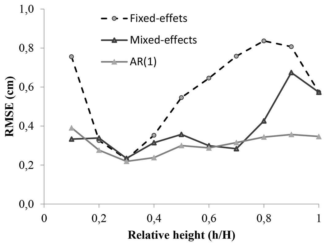
The lowest error value was obtained at 0.25-0.35, while the highest error value was 0.9 for relative length for the non-linear fixed-effect model. On the other hand, for the mixed effects models and AR(1) models of the same stem diameter model, the lowest error value for relative length was 0.3, while the highest was 0.9 (Tab. 4, Fig. 2). We found that the errors for the relative height values obtained using the AR(1) model were generally lower than those of the fixed and mixed effect models (Tab. 4, Fig. 2).
When examining the stem forms of Scots pine in the Ardahan region, we recorded that branching begins at about 70-80% of the tree height. As a consequence, the reliability of diameter estimates above these heights may decrease due to stem swelling.
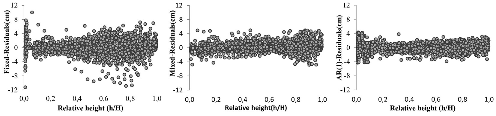
The distribution of errors in relative length estimates for the fixed and mixed-effect and AR(1) error structure of the Jiang et al. ([21])’s taper model are shown in Fig. 3. The model with AR(1) parameters showed the most homogeneous error variance structure at all relative height values. Moreover, the model with random effect parameters at all relative height values had a more homogeneous error variance structure than the nonlinear model. In other words, while the error variance values in the nonlinear model increased with increasing the relative height values, they remained constant in the mixed-effects and AR(1) models.
Fig. 3 - Residual plots for the fixed (left) and mixed (center) effects and AR(1) models (right).
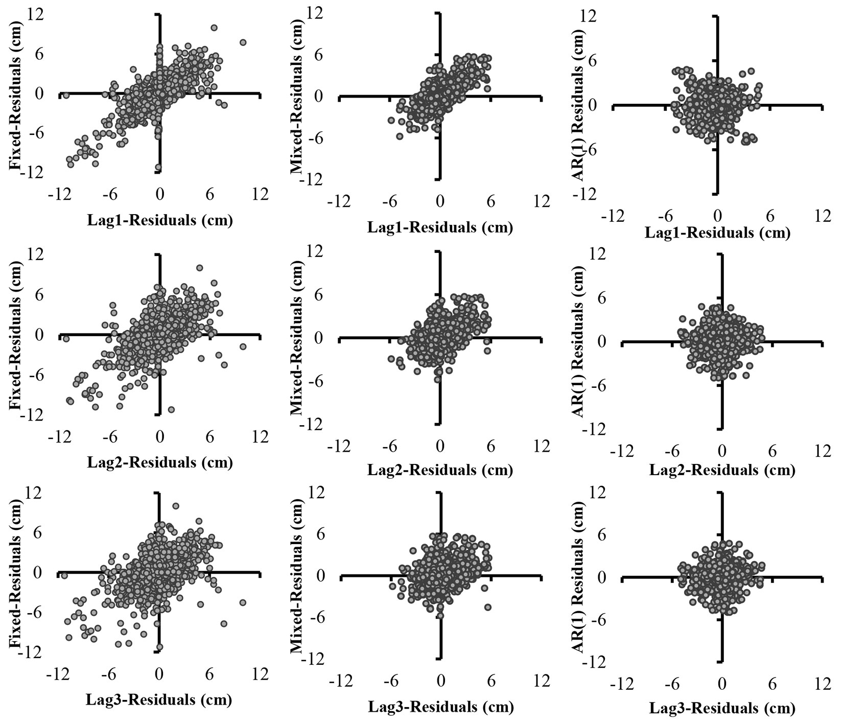
The autocorrelation of errors for the first three logs of the stem diameter model constructed for the Scots pine trees in Ardahan region is shown in Fig. 4. Here, a positive correlation was observed in the nonlinear regression model. However, the inclusion of the random effects parameters in the model did not completely solve the problem of autocorrelation of errors (Fig. 4). Previous studies showed that a mixed-effects model with random parameters may not be able to fully eliminate the error autocorrelation ([14], [47], [35], [20]). In this study, the use of the autoregressive error structure AR(1) fully removed the heteroscedasticity and autocorrelation in the residuals.
Fig. 4 - Residuals plotted against lagged residuals for fixed effects models (left column), mixed effects models (center column) and AR(1) models (right column).
Tab. 5shows the fitting results of the four stem volume models used for Scots pine in this study. Here, Model 1 ([21]) accounted for 99.10% of the variance in stem volume estimates, Model 4 ([13]) explained 98.03%, while Model 3 ([36]) and Model 2 ([32]) accounted for 97.67% and 97.66% of the total variance, respectively. Thus, the most successful model for stem volume development in Scots pine is the model developed by Jiang et al. ([21]), showing RMSE value of 0.1247 m3, ME value of 0.0070 m3, and MAE of 0.083 m3 (Tab. 5).
Tab. 5 - Fit statistics of the four stem volume equations used in this study.
| Model | Parameter | Jiang et al. ([21]) | Max & Burkhart ([32]) | Parresol et al. ([36]) | Fang et al. ([13]) |
|---|---|---|---|---|---|
| Fit data | ME | 0.01 | 0.01 | 0.08 | 0.07 |
| MAE | 0.08 | 0.10 | 0.12 | 0.11 | |
| RMSE | 0.12 | 0.18 | 0.20 | 0.18 | |
| R2adj | 0.99 | 0.98 | 0.98 | 0.98 | |
| Validation data |
ME | -0.03 | -0.02 | 0.06 | 0.04 |
| MAE | 0.07 | 0.11 | 0.10 | 0.09 | |
| RMSE | 0.11 | 0.17 | 0.16 | 0.14 | |
| R2adj | 0.99 | 0.98 | 0.98 | 0.99 |
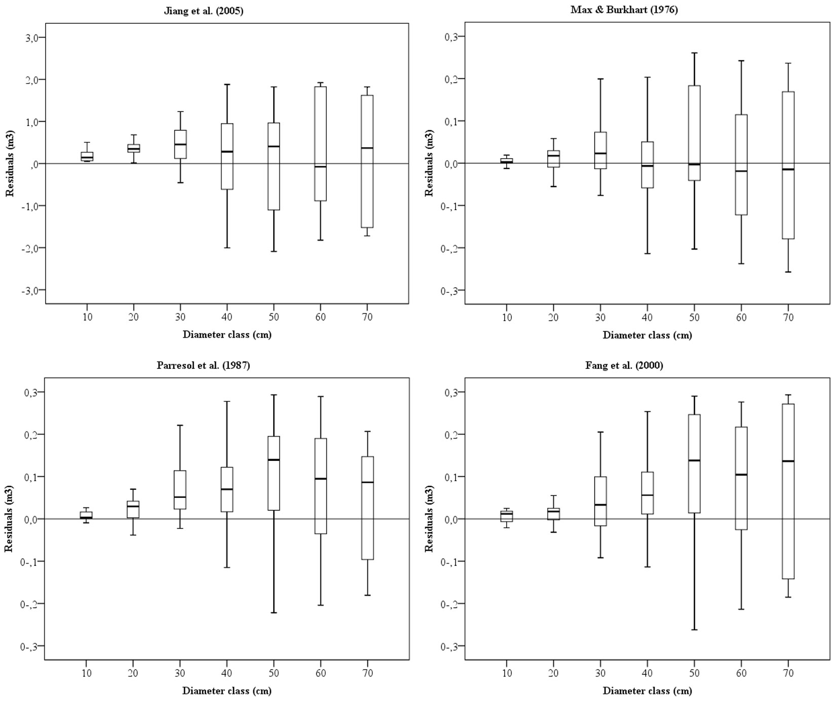
The boxplots of residuals in each diameter class for the four stem volume models are shown in Fig. 5. Model 1 ([21]) provided the lowest prediction errors for Scots pine trees. The deviation is generally lowest in the smallest diameter classes and highest in the medium-high diameter classes for all stem volume models (Fig. 5). Similar results are reported for several stem volume models studies by Barrio-Anta et al. ([4]), Zhao et al. ([51]), Hussain et al. ([19]), He et al. ([17]), Hirigoyen et al. ([18]). In any case, Jiang et al. ([21]) equation slightly underestimated the volume in the smallest diameter classes, overestimated in the largest diameter classes, and largely overestimated in the medium diameter classes. The other three equations used in this study generally underestimated the volume in all diameter classes.
Fig. 5 - Box plots of total volume residuals against diameter classes for Scots pine.
The suitability of the stem volume equations for the stand from which the samples were taken was tested using an independent data set ([28]). We applied the paired Student’s t-test to the validation data set (20% of the total data, 27 trees) to test the accuracy of stem volume predictions obtained by the four models (Tab. 1). The results showed that there was no significant differences between the observed and predicted values of stem volumes for all the models (Model 1: Student’s t=-0.739, p=0.467; Model 2: t=-0.528, p= 0.602; Model 3: t=-0.134, p=0.895; Model 4: t=-0.766, p=0.450). This indicates that the four stem volume models developed in this study are accurate and consistent with stands of pure Scots pine in the Ardahan region.
Conclusions
A compatible segmented taper model for pure Scots pine stands in the Ardahan region of Turkey was developed using the mixed-effects modeling approach and the AR(1) structure. Four segmented polynomial taper models were used to predict the variation of tree stem diameters. The stem taper equation developed by Jiang et al. ([21]) provided the most accurate predictions, accounting for 98.3% of the variance in the stem diameter estimate and showing a standard error of 1.955 cm.
Autocorrelation and heterogeneous distribution of error variance are common problems in models with hierarchical data structure. These problems cannot be eliminated in traditional regression models, but can be solved by the mixed-effects modeling approach and the autoregressive error structure AR(1), which represents the most important advantage of mixed-effects models over traditional regression models. In this study, the inclusion of random effects parameters to the model reduced the problem of error-related autocorrelation, resulting in a more homogeneous error variance structure in almost all relative height values and in a reduction of the RMSE values for both the AR(1) and mixed-effects models, compared with the nonlinear regression model. Finally, the autocorrelation problem was solved using the autoregressive error structure AR(1), as proven by the homogeneous error variance distribution.
Accurate and reliable assessments of tree or stand volume is highly dependent on the accuracy of stem taper estimation. In this study we showed that the estimation of stem taper in pure Scots pine stands of the Ardahan region can be successfully performed using nonlinear mixed-effects modeling technique, especially the AR(1) model, which provided accurate predictions within a wide range of diameter at breast height (6.0 to 75.0 cm) in Scots pine. However, when it comes to choose the best of various models with similar prediction success for a tree species in any region, the practical application of the method and the preferences of forest managers and practitioners should not be overlooked.
Acknowledgments
This study is part of the master’s thesis prepared by BS and supervised by AK for the Institute of Natural and Applied Sciences, Artvin Çoruh University, Turkey. The authors thank the other researchers involved in this study and the staff of Ardahan SFE.
Author contribution
BS and AK planned the experiments, contributed to data collection, data analysis and wrote the first draft. AK contributed to statistical analysis of the data, reviewed and edited the manuscript.
References
Gscholar
Gscholar
Gscholar
Gscholar
Gscholar
Gscholar
Gscholar
Gscholar
Gscholar
Authors’ Info
Authors’ Affiliation
Erzurum Regional Directorate Ardahan Forest District Directorate, 75000, Ardahan (Turkey)
Artvin Çoruh University Faculty of Forestry, Department of Forest Engineering, 08100, Artvin (Turkey)
Corresponding author
Paper Info
Citation
Saygili B, Kahriman A (2023). Modeling compatible taper and stem volume of pure Scots pine stands in Northeastern Turkey. iForest 16: 38-46. - doi: 10.3832/ifor4099-015
Academic Editor
Carlotta Ferrara
Paper history
Received: Mar 11, 2022
Accepted: Nov 07, 2022
First online: Jan 22, 2023
Publication Date: Feb 28, 2023
Publication Time: 2.53 months
Copyright Information
© SISEF - The Italian Society of Silviculture and Forest Ecology 2023
Open Access
This article is distributed under the terms of the Creative Commons Attribution-Non Commercial 4.0 International (https://creativecommons.org/licenses/by-nc/4.0/), which permits unrestricted use, distribution, and reproduction in any medium, provided you give appropriate credit to the original author(s) and the source, provide a link to the Creative Commons license, and indicate if changes were made.

Web Metrics
Breakdown by View Type
Article Usage
Total Article Views: 26362
(from publication date up to now)
Breakdown by View Type
HTML Page Views: 21162
Abstract Page Views: 2593
PDF Downloads: 2137
Citation/Reference Downloads: 0
XML Downloads: 470
Web Metrics
Days since publication: 1267
Overall contacts: 26362
Avg. contacts per week: 145.65
Article Citations
Article citations are based on data periodically collected from the Clarivate Web of Science web site
(last update: Mar 2025)
Total number of cites (since 2023): 1
Average cites per year: 0.33
Publication Metrics
by Dimensions ©
Articles citing this article
List of the papers citing this article based on CrossRef Cited-by.
Related Contents
iForest Similar Articles
Research Articles
Nonlinear mixed model approaches to estimating merchantable bole volume for Pinus occidentalis
vol. 5, pp. 247-254 (online: 24 October 2012)
Research Articles
Compatible taper-volume models of Quercus variabilis Blume forests in north China
vol. 10, pp. 567-575 (online: 08 May 2017)
Research Articles
Modelling taper and stem volume considering stand density in Eucalyptus grandis and Eucalyptus dunnii
vol. 14, pp. 127-136 (online: 16 March 2021)
Research Articles
Comparative analysis of taper models for Pinus nigra Arn. using terrestrial laser scanner acquired data
vol. 17, pp. 203-212 (online: 22 July 2024)
Research Articles
Analyzing regression models and multi-layer artificial neural network models for estimating taper and tree volume in Crimean pine forests
vol. 17, pp. 36-44 (online: 28 February 2024)
Research Articles
Stem profile of red oaks in a bottomland hardwood restoration plantation forest in the Arkansas Delta (USA)
vol. 15, pp. 179-186 (online: 19 May 2022)
Research Articles
The use of tree crown variables in over-bark diameter and volume prediction models
vol. 7, pp. 132-139 (online: 13 January 2014)
Research Articles
Modeling stand mortality using Poisson mixture models with mixed-effects
vol. 8, pp. 333-338 (online: 05 September 2014)
Research Articles
Estimation of stand crown cover using a generalized crown diameter model: application for the analysis of Portuguese cork oak stands stocking evolution
vol. 9, pp. 437-444 (online: 02 December 2015)
Research Articles
Total tree height predictions via parametric and artificial neural network modeling approaches
vol. 15, pp. 95-105 (online: 21 March 2022)
iForest Database Search
Search By Author
Search By Keyword
Google Scholar Search
Citing Articles
Search By Author
Search By Keywords
PubMed Search
Search By Author
Search By Keyword


