Stem profile of red oaks in a bottomland hardwood restoration plantation forest in the Arkansas Delta (USA)
iForest - Biogeosciences and Forestry, Volume 15, Issue 3, Pages 179-186 (2022)
doi: https://doi.org/10.3832/ifor4057-015
Published: May 19, 2022 - Copyright © 2022 SISEF
Research Articles
Abstract
Bottomland hardwoods are among the most diverse and productive forest ecosystems in the southeastern United States and are critically important for the provision of timber and non-timber ecosystem services. Red oaks, the dominant species in this group of forests, are of high ecological and economic value. Stem profile models are essential for accurately estimating the merchantable volume of oak trees, which is also closely indicative of total tree biomass and other ecosystem services given their allometric relationships. This study aims to develop and compare stem profiles among three red oak species in an 18-year old plantation forest using destructive sampling. Sixty trees randomly selected from an oak restoration plantation in the Arkansas Delta were felled for measuring the diameter-outside-bark (DOB) and diameter-inside-bark (DIB) at different stem heights. These sample composed of twenty trees from each of three species: cherry bark oak (CBO - Quercus pagoda Raf), Nuttall oak (NUT - Quercus texana Buckley), and Shumard oak (SHU - Quercus shumardii Buckl). Multiple models, including the segmented-profile model, form-class profile model, and second-and third-order polynomial models were fitted and compared. Results demonstrate that the form-class profile model was the best fitted for CBO and NUT, whereas the third-order polynomial model was the best for SHU. CBO tends to grow taller and has a higher wood density than NUT and SHU. These findings will inform restoration and management decisions of bottomland hardwood forests, especially red oaks in the region.
Keywords
Cherry Bark Oak, Nuttall Oak, Shumard Oak, Taper Models, Wood Density, Southeastern United States
Introduction
Bottomland hardwoods are among the most diverse and productive forest ecosystems in the southeastern US. They are critically important for providing many benefits including timber, water regulation, wildlife habitats and biodiversity, natural sceneries, and carbon sequestration and storage, among others ([38], [18], [9]). This group of forests once covered nearly 12 million ha in the region; however, sixty percent of bottomland hardwood forests have been lost in the past two hundred years mainly due to agricultural expansion ([9]). Extensive efforts have been undertaken to restore bottomland hardwood forests in recent decades, mainly through plantations on cropland that was originally converted from forests ([2]). Among the most important tree species in this ecosystem are oaks, particularly red oaks ([2], [18], [23]), which provide food for a variety of wildlife and lumber and veneer for the production of high quality furniture, flooring, and other products. Yet, the availability of accurate growth and yield models for the forests in general and oaks in particular is limited compared to other commercial species like pines ([35]). Information on young oak stand development is particularly limited. Such limitations have hindered the development and implementation of effective forest restoration and management decisions to enhance the provisions of timber and non-timber ecosystem services from this group of forests ([25], [36]).
Stem profile studies can help improve the accuracy of growth and yield estimations and projections while providing valuable information about the characteristics of trees and forests. Tree profile equations estimated statistically using empirical data predict the diameter at various heights along the bole of a tree ([28], [32]), improving volume and carbon estimates. Profile equations allow for predicting volumes to merchantable top diameters, a fundamental basis for forest managers to compute volumes to any top diameter as well as diameter/height at a specific height/diameter along the stem. However, there is a lack of published profile equations for oaks in the hardwood forests. Given the ecological importance of oaks in the forests and the high value of oak wood products, the development of profile equations will aid in their volume and value estimation.
Profile modeling is an active area of research in forestry given the flexibility and utility afforded by the various existing models ([45], [42]). Taper equations represent the mathematical expression of stem diameter change with respect to height on the basis of species, age, and stand condition ([16], [4]). A number of taper functions have been developed for different tree species with various forms including simple taper functions, variable-form taper functions, and segmented polynomial taper functions ([28], [17]). Simple taper functions mainly define tree profiles with a single continuous equation for the whole bole ([5], [19], [31], [15], [11], [47]). Though simple, they were unable to precisely describe the whole bole profile especially the base of the stem ([17]). By contrast, the variable-form taper functions assume that the stem form/shape continuously changes with the height ([21]); therefore, those equations describe the stem profile with an exponent variable to characterize the neiloid, paraboloid, and conic ([30], [20]). The advantages of the variable-form taper functions are that they describe the stem form through a continuous function and can predict/estimate the upper-stem diameters more accurately. However, the disadvantage of these functions are their inability to be logically associated to estimating total volumes.
Segmented polynomial taper functions describe stem shape through fitting a distinct equation for each segment and then binding multiple equations together to produce and overall segmented structure estimation ([27], [6], [8], [17]). Max & Burkhart ([27]) developed a well-known profile equation for loblolly pine (Pinus taeda) involving a segmented polynomial regression approach, which delineates the bole of a tree into three sections based on the generalized relative geometric form. This approach is based on the assumption that in mathematical evaluation a segmented model will best approximate the stem form. A segmented polynomial profile model can be created by grafting three sub-models at two joint points referred to as inflection points ([40]). Similar to Max & Burkhart ([27]) model, Cao ([7]) segmented profile model also consists of three sub-models that are joined at two points; each sub-model in Cao ([7]) has a form of the modified Goulding & Murray ([13]) model, which can be inverted to predict height and volume. Clark et al. ([8]) proposed a form-class segmented profile model by incorporating the form quotient of the Girard form class to produce a more robust model. Their model assesses stem structure partially based on the relative measurements involved with the quotient. They compared their model with Max & Burkhart ([27]) segmented polynomial equation and found that the form-class segmented model provides more accurate volume estimations. The segmented-profile models including form-class segmented profile models were commonly employed in fitting the stem of hardwood species. For example, Jiang et al. ([17]) employed the segmented-profile model by Max & Burkhart ([27]) and Clark et al. ([8]) in fitting the stem of yellow-poplar; Tian et al. ([42]) fitted the invasive tallow stem using both Max & Burkhart ([27]) and Cao ([7]) as well as Clark et al. ([8]). In addition, Alkan & Ozçelik ([1]) tested nine taper equations for stem profile and volume of Taurus fir in Taurus Mountains of Turkey and found that among segmented taper models, the Fang et al. ([10]) model was the most accurate taper equation for estimating diameter, predicting merchantable, and total volume. Moreover, this model does not require numerical integration like the variable-form equations for volume estimations. Parker ([34]) suggested the use of a non-segmented, third degree polynomial for small data sets with limited diameter and height ranges, and developed a computer program for calculating both non-segmented and single or multiple segmented tree profile equations. His equations were based on non-destructive measurements of upper stem diameters of standing trees taken with an optical dendrometer. Overall, segmented polynomial functions composed of a series of sub-models representing various sections of the stem perform better than simple or variable form taper functions and are widely used ([32]).
The main objective of this study is to develop and compare the stem profile models for three oak species planted in the Arkansas Delta, located in the lower Mississippi River alluvial valley (LMRAV). Hardwood forests in the LMRAV are a typical example of bottomland hardwood forests in the southeastern US in terms of their ecological features, conversion to croplands, and restoration efforts ([24], [2]). The three oak species are cherry bark oak (CBO - Quercus pagoda Raf), Nuttall oak (NUT - Q. texana Buckley), and Shumard oak (SHU - Q. shumardii Buckl). Different profile models for each species will be estimated and compared. Additionally, wood density will also be measured and compared among the three oak species, indicative of the physical property and carbon content of the oak wood. As natural and primary hardwood forests become increasingly scarce and are protected for conservation purposes, a dominant amount of hardwood timber has come from second growth and plantations. Plantations will become increasingly important in timber supply in the near future. Additionally, stem profile equations are fundamental to quantifying tree biomass which is closely related to the provisions of non-timber ecosystem services. Hence, the results of this study will inform decision making in oak plantation design and management to restore the bottomland hardwood forests for both timber and non-timber objectives while enriching the existing literature in oak stem profile, volume, and wood density.
Methodology
Study site
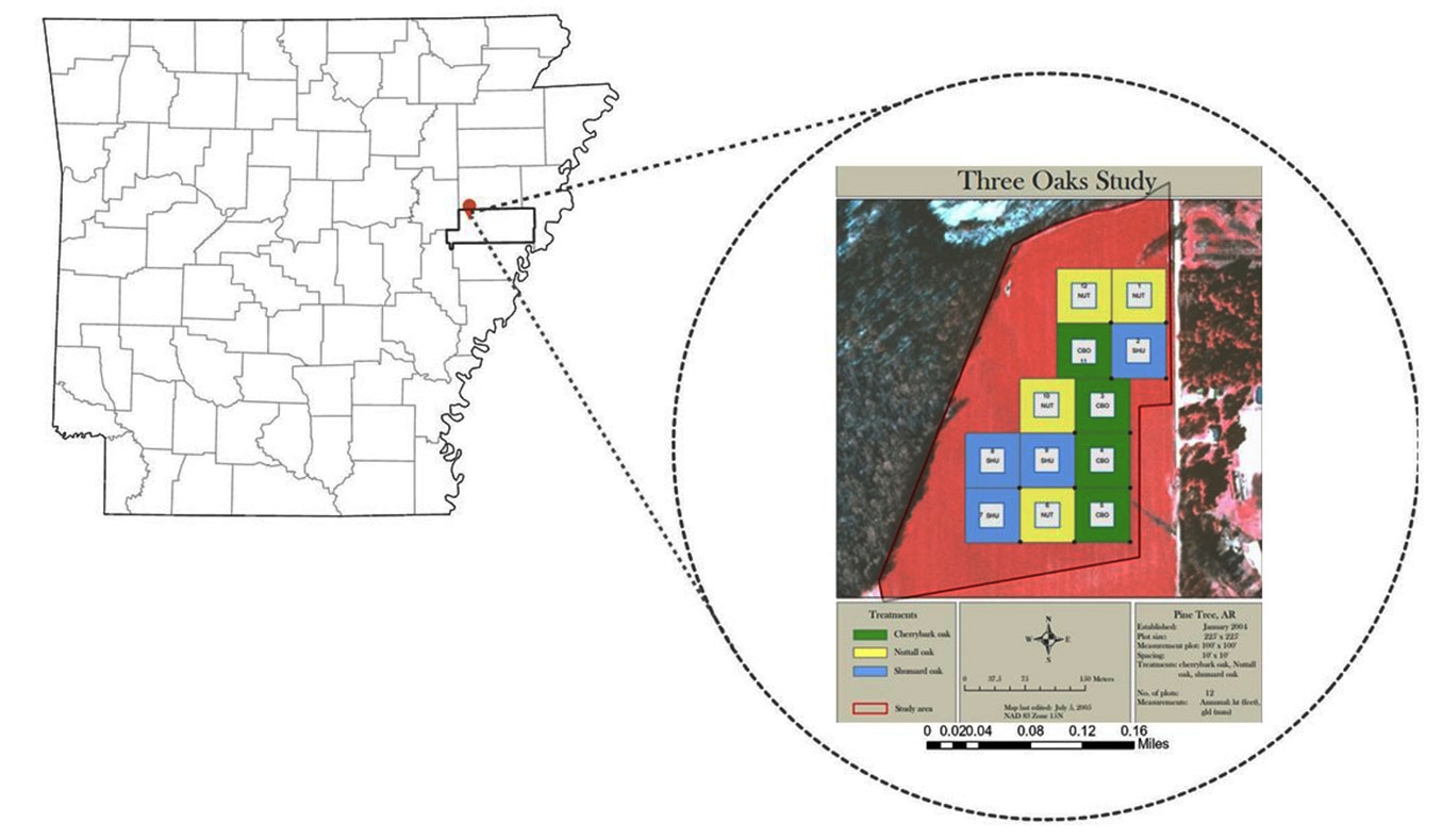
The data for this study were collected from an oak restoration plantation established at the University of Arkansas Division of Agriculture Pine Tree Research Station (AgPTRS) in the Arkansas Delta (35° 07′ 48″ N, 90° 55′ 45″ W). The 12.15 ha hardwood plantation was on a prior flood prone and low productive bean field that was enrolled in the Conservation Reserve Program. The oak trees involved in this study were planted in February 2004 after the site was ripped to a depth of 0.91 m in November 2003. Seedlings were hand planted at a 3.05 × 3.05 m spacing in 12 plots with 4 replications. Each of the three red oak species (cherry bark oak, CBO - Quercus pagoda Raf; Nuttall oak, NUT - Quercus texana Buckley; and Shumard oak, SHU - Quercus shumardii Buckl) were randomly assigned to 68.58 × 68.58 m plots. (Fig. 1). No further management was applied to the plots in the 18-year interval between planting and data collection for this study.
Fig. 1 - Study site and the layout of the measurement plots with all three oak species.
Data collection
Destructive sampling procedures are a standard practice in tree profile data collection because stem diameters including diameter-outside-bark (DOB) and diameter-inside-bark (DIB) can easily be measured on felled trees. In addition, stem profile data measured along a felled tree provides reliable data, representing one of the most accurate methods for volume quantification. We employed destructive sampling for accurate and reliable profile data measurements of diameter and height value pairs along the entire length of the tree stem.
A total of 60 oak trees were randomly selected (20 for each species of CBO, NUT, and SHU) equally from all each of the four replications in the study (5 trees from each replication). Prior to felling, total height of the standing sample trees was measured with a clinometer; meanwhile, diameter at breast height (DBH) were also measured for all the 60 selected trees. They were then felled at approximately 0.15 m from the ground, and the bole was cleared of branches to facilitate measurements. Merchantable stem length was recorded for each tree by running a tape measurement along the length of the main apical branch until a 10.16 cm DOB was reached. The stem was divided into 1.83 m sections in the field and disks with 2.5-5.0 cm in thickness were then extracted from the midpoint of each section; DOB and DIB were measured at the lower and upper ends of each section. These collected disks were marked with species, tree number as well as disk number. They were sealed in pre-weighed and marked plastic bags to preserve their green weight. In addition, both DOB and DIB at a selected height (~5.27 m) was also recorded. As a result, DOB and DIB were recorded along the bole at relative heights of 0.15 m, 1.37 m, 1.83 m, 3.66 m, 5.27 m, 5.49 m, 7.32 m etc. until the point of a 10.16 cm diameter outside bark was reached. At each recorded height along the felled stem, both DOB and DIB were measured twice in two different directions for accuracy.
The tree disks were returned to the laboratory and weighed in the pre-weighed bags to determine green weight. The disks were then oven dried at 80 °C and reweighed to determine moisture content. A wedge of wood was then separated from the oven dry disk and the weight of that wedge was recorded. The volume of the wedge was then determined by the displacement method in water at 3 °C after coating the wedge in paraffin wax. The wood density was computed using the dry weight of the wedge divided by the volume of the same wedge, denoted by grams per cubic centimeter (g cm-3).
Profile models
A total of seven profile models were fitted in this study including the segmented polynomial models of Max & Burkhart ([27]), Cao ([7]), Clark et al. ([8]) and optimized Cao ([7]); and the form-class models of second- and third-order polynomial equations. To be specific, those seven profile models were: (MB) Max & Burkhart ([27]); (CAO) Cao ([7]); (CSS) Clark et al. ([8]), optimized Cao ([7]); (OCAO_F) modified MB to pass through DBH and FC at FC height, optimized Cao ([7]); (OCAO_R) modified MB to pass through DBH and FC at relative height; (POLY3) 3rd-order polynomial joined at breast height to 5th order polynomial; and (POLY2) 2nd-order polynomial joined at breast height to 5th-order polynomial. Specific mathematic expressions of these models are shown in the equations below. The notations associated with the seven taper equations are listed in Tab. 1.
Tab. 1 - Notations associated with stem profile models.
| Notations | Definition |
|---|---|
| TH | The total height of a tree |
| h D | Breast height (1.37 m) |
| D | Diameter at breast height (DBH) |
| d | Diameter at specific height of h, including diameter-outside-bark (DOB) and diameter-inside-bark (DIB) |
| h | Height above the ground to the measurement point |
| d * | Calibrated diameter |
| F | diameter at 5.27 m, including DOB and DIB |
The widely used MB profile function is expressed in eqn. 1 and b1, b2, b3, b4, α, and β are parameters to be estimated, α and β represent the joint points as showed in the constraint conditions function. This segmented polynomial model describes a tree stem with three sections (eqn. 1):
where S = (h/TH) and S2 = (h)2/(TH)2. The constraint conditions for this model are (eqn. 2):
The profile model of CAO including the optimized OCAO_F and OCAO_R ([7]) is shown in eqn. 3-5 with parameter b1 being modified to parameter b1* for OCAO_R (eqn. 3, eqn. 4, eqn. 5):
where S3 = 4.5/TH.
The segmented model of CSS describes the stem with four sections composed of the butt section (from stump to breast height of 1.37 m), lower stem (between 1.37 m and 5.27 m), middle stem (from 5.27 m to 40-70% of total height), and upper stem (from 40% to 70% of total height to the tip of the tree - [17], [33]). The mathematic expression is presented in eqn. 9, where b1, b2, b3 are the parameters for the butt section; b4 is the parameter for the lower stem; b5, b6 are the coefficients for height above 5.27 m; Z1 = 1-(h/TH) = 1 - S; Z2 = 1-(4.5/TH) = 1 - S3, Z3 = (h-17.3)/(H-17.3).
Hence, the constraints for this model are (eqn. 10):
By contrast, the form-class models of second- and third-order polynomial models are shown in eqn. 11 and eqn. 12, respectively:
where b1, b2, b3, b4, b5 are the parameters to be estimated.
Statistical analysis
To test for differences in DBH and total height of CBO, NUT, and SHU at a 0.05 significance level, analysis of variance (ANOVA) was employed.
The measurements of DOB, DIB, and height pairs provided the inputs for TProfile ([26]) to estimate the parameters of each profile equation described above. All profile equations fitted in this study were calculated using Tprofile which can fit commonly used profile functions for a variety of hardwood species throughout the Southeast US ([26], [12]). One potential problem in fitting the stem profile model is autocorrelation ([43], [46]); to address this concern, Durbin-Watson test for both DOB and DIB data of three oak species were performed. The test statistic values were all around 1.4/1.5 (p-value ~ 0.09), indicating that autocorrelation was not a major concern in the data.
Those fitted equations were evaluated and compared using mean absolute error (MAE), root mean square error (RMSE), and the index of fit (FI). Specifically, the MAE (eqn. 13) was computed along the bole as the average absolute difference between observed and predicted diameter values. The RMSE (eqn. 14) was calculated by the square root of the average of the absolute value of the squared biases whereas FI (eqn. 15) was calculated as one minus the sum of squared errors divided by the total sum of squares.
where Yi denotes the observations/measurements, Ŷi represents the predictions, bar{Y} is the mean of Yi, and n is the number of observations in the dataset.
Furthermore, we plotted the residuals (computed by observed values minus predicted values) of DOB and DIB against relative height to diagnose how well each model predicted the stem profile data. Together with the computed RMSE and FI values, we determined the best fit profile equation for each oak species.
Results
Descriptive statistics for three oak species
The descriptive statistics of DBH, total height, and wood density for all three oak species of CBO, NUT, and SHU are summarized in Tab. 2. Average DBH for CBO, NUT, and SHU were 18.44 cm, 16.51 cm, and 16.61 cm, respectively. Total height, on average, was 17.75 m, 15.56 m, and 13.58 m respectively for CBO, NUT, and SHU. The results of ANOVA tests indicated that there was no distinct difference in DBH among CBO, NUT, and SHU; however, a significant difference was found in total height among them. To be specific, CBO was significantly taller than NUT which was taller than SHU, though they were planted in a similar environment at the same time. NUT and SHU have a similar wood density, which is significantly lower than that of CBO.
Tab. 2 - Descriptive statistics of DBH and total tree height for CBO, SHU, and NUT. Different letters in each column indicate statistically different values (p<0.05). (CBO): cherry bark oak (Quercus pagoda Raf); (NUT): Nuttall oak (Quercus texana Buckley); (SHU): Shumard oak (Quercus shumardii Buckl); (n): sample size; (SD) standard deviation.
| Oak species (n) | Statistics | DBH (cm) |
Total Height (m) |
Wood density (g cm-3) |
|---|---|---|---|---|
| CBO (20) |
Average | 18.44a | 17.75a | 0.73a |
| Min | 13.72 | 15.24 | 0.65 | |
| Max | 23.11 | 19.81 | 0.86 | |
| SD | 2.67 | 1.09 | 0.05 | |
| NUT (20) |
Average | 16.51a | 15.56b | 0.68b |
| Min | 11.68 | 12.19 | 0.49 | |
| Max | 20.60 | 18.29 | 0.83 | |
| SD | 2.59 | 1.48 | 0.07 | |
| SHU (20) |
Average | 16.61a | 13.58c | 0.68b |
| Min | 11.05 | 11.28 | 0.59 | |
| Max | 26.67 | 16.46 | 0.77 | |
| SD | 4.39 | 1.34 | 0.04 |
Profile equation parameters and comparisons
Tprofile estimated parameters for all seven profile models for the three oak species. Tab. S1 (Supplementary material) summarizes parameter estimations of all fitted profile models for both DOB and DIB of each oak species and the number of observations for each model. According to the MAE (lower), RMSE (lower), and FI (higher - Tab. 3) along with graphical evaluation of residual plots (Fig. S1a-S1c in Supplementary material), the CSS profile model was the best fitted for both CBO and NUT; however, the third-order polynomial model (POLY3) was the best fitted for SHU, especially in terms of DIB. Specifically, the FI, MAE, and RMSE for both DOB and DIB of CBO were FIOB/IB = 0.987, MAEOB/IB = 0.025, and RMSEOB/IB = 0.094 with the CSS model; whereas for NUT with the CSS model, the FI, MAE, and RMSE were estimated at FIOB = 0.973, MAEOB = 0.033, and RMSEOB = 0.145 for DOB and at FIIB = 0.967, MAEIB = 0.033, and RMSEIB = 0.150 for DIB, respectively. By contrast, the FI, MAE, and RMSE for SHU with the POLY3 model were estimated at FIOB = 0.976, MAEOB = 0.041, and RMSEOB = 0.140 for DOB, and FIIB = 0.968, MAEIB = 0.064, and RMSEIB = 0.152 for DIB. To be noted, the MAE of CSS for both DOB and DIB profile of CBO species was slightly higher than the MB model (MAEMB_OB = 0.023, MAEMB_IB = 0.015) while it was slightly higher than the CAO model (MAECAO_OB = 0.028) for DOB profile of NUT. In addition, there was no difference in FI and RMSE for SHU between the POLY3 and CSS models for DOB. Yet, there was a slight difference in FI and RMSE for the DIB profile of SHU between the two models with FIIB = 0.966 and RMSEIB = 0.155 for the CSS model. Tab. S1 (Supplementary material) summarizes the parameters estimated for all seven models for both DOB and DIB profiles together with the total number of observations utilized in the model fitting; Tab. 3summarized all the statistics of model evaluation.
Tab. 3 - Model evaluation statistics of MAE, EMSE, and FI of seven profile models for oak species of CBO, NUT, and SHU. (CBO): cherry bark oak (Quercus pagoda Raf); (NUT): Nuttall oak (Quercus texana Buckley); (SHU): Shumard oak (Quercus shumardii Buckl); (MB): Max & Burkhart ([27]); (CAO); Cao ([7]); (CSS) Clark et al. ([8]); (OCAO_F): optimized Cao ([7]) modified MB to pass through DBH and FC at FC height; (OCAO_R): optimized Cao ([7]) modified MB to pass through DBH and FC at relative height; (POLY3): 3rd-order polynomial joined at breast height to 5th-order polynomial; (POLY2): 2nd-order polynomial joined at breast height to 5th-order polynomial; (DIB): diameter-inside-bark; (DOB): diameter-inside-bark.
| Model | Oak species Statistics | CBO | NUT | SHU | |||
|---|---|---|---|---|---|---|---|
| DOB | DIB | DOB | DIB | DOB | DIB | ||
| MB | RMSE | 0.117 | 0.109 | 0.234 | 0.229 | 0.183 | 0.188 |
| MAE | 0.023 | 0.015 | 0.033 | 0.036 | 0.089 | 0.089 | |
| Index of Fit | 0.979 | 0.979 | 0.930 | 0.925 | 0.958 | 0.951 | |
| CAO | RMSE | 0.135 | 0.122 | 0.224 | 0.244 | 0.196 | 0.028 |
| MAE | 0.071 | 0.056 | 0.028 | 0.117 | 0.140 | 0.254 | |
| Index of Fit | 0.973 | 0.975 | 0.934 | 0.914 | 0.953 | 0.891 | |
| CSS | RMSE | 0.094 | 0.094 | 0.145 | 0.150 | 0.140 | 0.155 |
| MAE | 0.025 | 0.025 | 0.033 | 0.033 | 0.089 | 0.091 | |
| Index of Fit | 0.987 | 0.987 | 0.973 | 0.967 | 0.976 | 0.966 | |
| OCAO_F | RMSE | 0.109 | 0.104 | 0.201 | 0.236 | 0.157 | 0.221 |
| MAE | 0.051 | 0.043 | 0.074 | 0.178 | 0.079 | 0.157 | |
| Index of Fit | 0.982 | 0.981 | 0.947 | 0.920 | 0.970 | 0.932 | |
| OCAO_R | RMSE | 0.099 | 0.086 | 0.173 | 0.191 | 0.140 | 0.208 |
| MAE | 0.036 | 0.028 | 0.048 | 0.071 | 0.081 | 0.160 | |
| Index of Fit | 0.985 | 0.986 | 0.958 | 0.945 | 0.974 | 0.934 | |
| POLY3 | RMSE | 0.102 | 0.104 | 0.191 | 0.229 | 0.140 | 0.152 |
| MAE | 0.041 | 0.030 | 0.036 | 0.074 | 0.041 | 0.064 | |
| Index of Fit | 0.984 | 0.984 | 0.953 | 0.940 | 0.976 | 0.968 | |
| POLY2 | RMSE | 0.104 | 0.109 | 0.188 | 0.206 | 0.140 | 0.152 |
| MAE | 0.043 | 0.036 | 0.036 | 0.079 | 0.046 | 0.064 | |
| Index of Fit | 0.984 | 0.982 | 0.953 | 0.939 | 0.976 | 0.967 | |
In addition, model performance was further evaluated using average residual plots for all seven models of three oak species (see Fig. S1-S3 in Supplementary material). In these plots, the y-axis represents the average residues and x-axis represents the relative height, h/TH. By comparing seven average residual curves for each species, we found that the best fitted model for both CBO and NUT was the CSS model while POLY3 is the best for SHU.
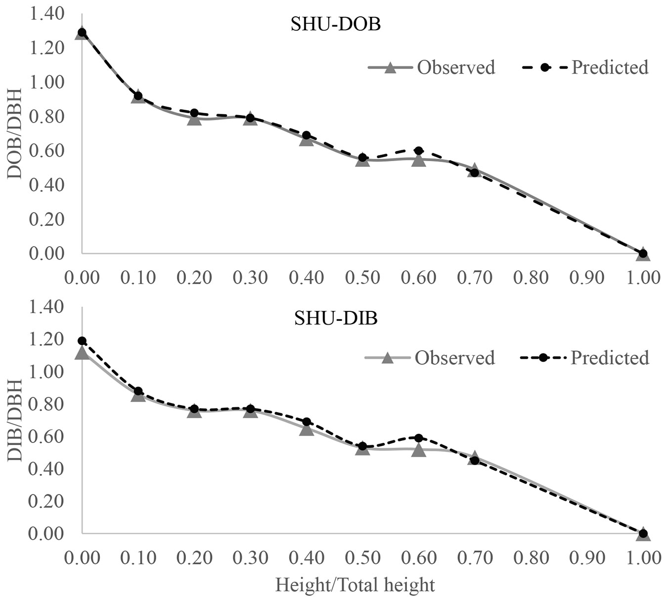
Finally, graphical profile comparisons were also made to visualize the difference between the average observed and predicted stem forms with 0.1 relative height interval (Fig. 2, Fig. 3, Fig. 4). We constructed the stem profile curves for both DOB and DIB for each species using its best fitted profile equations and the measurement data. Those curves also demonstrated that there was a good fit between the observed and predicted stem diameter values along the stem, which in turn confirmed that those profile equations were able to accurately predict the stem profile.
Fig. 2 - DOB and DIB profiles for cherry bark oak (CBO) using the best fitted model of CSS ([8]).
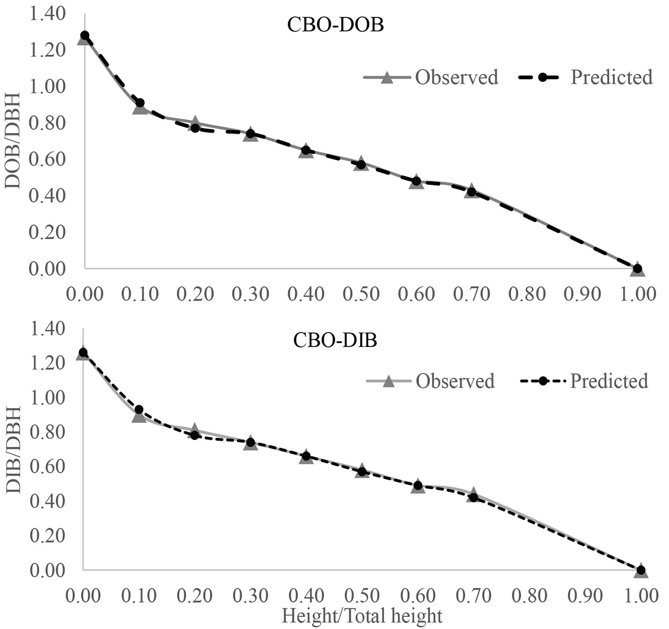
Fig. 3 - DOB and DIB profiles for Nuttall oak (NUT) using the best fitted model of CSS ([8]).
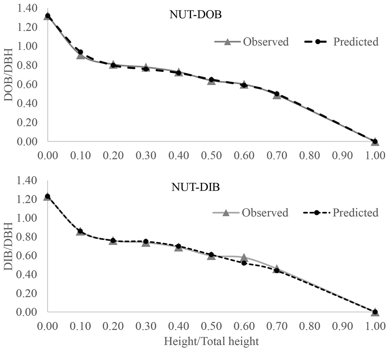
Fig. 4 - DOB and DIB profiles for Shumard oak (SHU) using the best fitted model of POLY3 (3rd-order polynomial joined at breast height to 5th-order polynomial).
Discussion
As explained by Avery & Burkhart ([3]), numerous factors could affect the performance of profile equations, including species, region, number of sample trees, data collection method among others. Those factors were all carefully considered and taken into account in the development of oak profile equations in this study. As reported by Saarinen et al. ([37]), the sample size of destructive stem analysis could affect parametrizing the stem profile equations. A total sample of 60 oak trees, with 20 trees for each species, is considered to be an appropriate sample size for this study given that all oak trees were felled on the same even-aged restoration plantation site. However, since the data comes from a single site, the effect of geographical variability is not addressed. Variables including total height, DBH, various heights along the stem, and DOB and DIB at different heights were measured using the destructive sampling method. This procedure provided reliable data for fitting the oak profile models. Seven different profile models were estimated and compared for each oak species. Multiple indicators including RMSE, index of fit, and residual plots were used to diagnose the fitted models, representing a statistically sound approach for model evaluation.
Our results show that the best fitted model was CSS for both CBO and NUT, whereas it was POLY3 for SHU. Although no difference was found between CSS and POLY3 for fitting the DOB profile of SHU, for the DIB profile of SHU the FI of the CSS model was slightly lower than that of POLY3, while the RMSE of the CSS model was slightly higher than that of POLY3. As reported by Muhairwe et al. ([29]), species could be an influencing factor for stem form variation. The MB model did not exhibit better performance than CSS. This may be partly because the MB model is constrained by a lack of representation of upper stem diameter, which is evidenced by an insufficient number of observations in the upper crown area. Moreover, the most important advantage of Clark et al. ([8]) is using extra upper diameter measurement at 5.27 m which also contributed to the model performance. Leites & Robinson ([22]) reported that crown dimension is another potential factor that contributes to the differences of stem profile. Therefore, future work can incorporate crown length and crown ratio into the profile models. In addition, utilization of modern regression techniques such as the mixed-effects modeling approach can also improve the profile model performance. For example, Gómez-García et al. ([14]) developed a mixed-effect variable exponent taper equation for birch trees in northwestern Spain which produced the best fitting statistics. The profile equations that express mathematical relationships between tree height and diameter are essential for quantifying stem volume as well as total tree biomass and carbon content. Based on the profile equations, stem volume can then be calculated ([44]). With properly estimated allometric relationships between the volumes of stem and other parts of the tree, total tree biomass and carbon content can also be derived. Besides, the similarities and differences in DBH and total heights among the three species can aid in selecting a proper species mix to achieve different management objectives. For example, Cherry bark oak is a better species choice than Nuttall or Shumard oak if the management objective is for timber, biomass, or carbon because cherry bark oak grows taller and has a higher wood density than Nuttall or Shumard oak, although they have similar DBH at the same age ([41]). However, because of their different heights, the mix of the three species can create more diverse stand structure and enhance biodiversity. Thus, our results provide a base-station for guiding the restoration and management of bottomland hardwood plantation forests to achieve both timber and non-timber objectives.
Conclusions
We estimated stem profile models for three red oak species (cherry bark, Nuttall, and Shumard oaks) with data collected from 60 felled trees randomly selected from a plantation in the Arkansas Delta in the southern United States. We found the best fitted model was Clark et al. ([8]) profile equation for cheery bark and Nuttall oaks and the third-order polynomial model for Shumard oak. Additionally, there is no statistically significant difference in DBH among the three oak species while cherry bark oak is the tallest and has the highest wood density of the three species. The fitted profile equations in this study can be implemented into inventory software such as TCruise ([26]) to improve the stem volume estimates of young oak trees in Arkansas Mississippi Delta. Given that an increasing amount of hardwood timber is supplied from second growth and plantations, our findings will guide decision making in red oaks restoration and management and their wood product marketing. Moreover, our estimated stem profile models and wood density can help quantify total tree biomass and associated carbon content. This, however, will entail the development of allometric relationships between the volumes or biomass quantities of stem and other parts of trees such as branches, leaves, and roots. Future studies on this site will determine if the stem profiles change over time as this plantation matures.
A few caveats of this study should be noted. First, while the results of fitted profile models provide a guideline for estimating the stem volume of oak species, we do not include comparisons with oak volume models given that the focus of this study was to compare stem profiles among different oak species grown on the same site instead of volume prediction. Second, the data were collected from an even-aged plantation and could not symbolize to other natural/planted mixed species and uneven-aged bottomland hardwood forests in this region, further study is needed to assess the viability of widespread application.
Acknowledgments
We are thankful for the support provided by the College of Forestry, Agriculture & Natural Resources at the University of Arkansas at Monticello and the Arkansas Center for Forest Business in completing this study. We also thank Ouname Mhotsha for helping data collection, and Ruxin Tao for his suggestion in making the study site map. Additionally, we are grateful for all field supports including technical and equipment support provided by the Division of Agriculture Pine Tree Research Station.
References
Gscholar
Gscholar
Gscholar
Gscholar
Gscholar
Gscholar
Gscholar
Authors’ Info
Authors’ Affiliation
Matthew Pelkki 0000-0002-4588-1310
Arkansas Forest Resources Center, College of Forestry, Agriculture & Natural Resources, University of Arkansas at Monticello, Monticello, AR 71656-3468 (USA)
Department of Ecology and Conservation Biology, Texas A&M University, College Station, TX 77843 (USA)
Corresponding author
Paper Info
Citation
Tian N, Gan J, Pelkki M (2022). Stem profile of red oaks in a bottomland hardwood restoration plantation forest in the Arkansas Delta (USA). iForest 15: 179-186. - doi: 10.3832/ifor4057-015
Academic Editor
Agostino Ferrara
Paper history
Received: Jan 05, 2022
Accepted: Apr 05, 2022
First online: May 19, 2022
Publication Date: Jun 30, 2022
Publication Time: 1.47 months
Copyright Information
© SISEF - The Italian Society of Silviculture and Forest Ecology 2022
Open Access
This article is distributed under the terms of the Creative Commons Attribution-Non Commercial 4.0 International (https://creativecommons.org/licenses/by-nc/4.0/), which permits unrestricted use, distribution, and reproduction in any medium, provided you give appropriate credit to the original author(s) and the source, provide a link to the Creative Commons license, and indicate if changes were made.

Web Metrics
Breakdown by View Type
Article Usage
Total Article Views: 31697
(from publication date up to now)
Breakdown by View Type
HTML Page Views: 26985
Abstract Page Views: 2376
PDF Downloads: 1784
Citation/Reference Downloads: 1
XML Downloads: 551
Web Metrics
Days since publication: 1513
Overall contacts: 31697
Avg. contacts per week: 146.65
Article Citations
Article citations are based on data periodically collected from the Clarivate Web of Science web site
(last update: Mar 2025)
Total number of cites (since 2022): 2
Average cites per year: 0.50
Publication Metrics
by Dimensions ©
Articles citing this article
List of the papers citing this article based on CrossRef Cited-by.
Related Contents
iForest Similar Articles
Research Articles
Compatible taper-volume models of Quercus variabilis Blume forests in north China
vol. 10, pp. 567-575 (online: 08 May 2017)
Research Articles
Effect of stand density on longitudinal variation of wood and bark growth in fast-growing Eucalyptus plantations
vol. 12, pp. 527-532 (online: 12 December 2019)
Research Articles
Variation of wood and bark density and production in coppiced Eucalyptus globulus trees in a second rotation
vol. 9, pp. 270-275 (online: 08 September 2015)
Research Articles
Modelling taper and stem volume considering stand density in Eucalyptus grandis and Eucalyptus dunnii
vol. 14, pp. 127-136 (online: 16 March 2021)
Research Articles
Comparative analysis of taper models for Pinus nigra Arn. using terrestrial laser scanner acquired data
vol. 17, pp. 203-212 (online: 22 July 2024)
Research Articles
Analyzing regression models and multi-layer artificial neural network models for estimating taper and tree volume in Crimean pine forests
vol. 17, pp. 36-44 (online: 28 February 2024)
Research Articles
The use of tree crown variables in over-bark diameter and volume prediction models
vol. 7, pp. 132-139 (online: 13 January 2014)
Research Articles
Hygroscopicity of the bark of selected forest tree species
vol. 10, pp. 220-226 (online: 06 November 2016)
Commentaries & Perspectives
Benefits of a strategic national forest inventory to science and society: the USDA Forest Service Forest Inventory and Analysis program
vol. 1, pp. 81-85 (online: 28 February 2008)
Research Articles
Comparison of extractive chemical signatures among branch, knot and bark wood fractions from forestry and agroforestry walnut trees (Juglans regia × J. nigra) by NIR spectroscopy and LC-MS analyses
vol. 15, pp. 56-62 (online: 08 February 2022)
iForest Database Search
Search By Author
Search By Keyword
Google Scholar Search
Citing Articles
Search By Author
Search By Keywords
PubMed Search
Search By Author
Search By Keyword


