A geographically weighted deep neural network model for research on the spatial distribution of the down dead wood volume in Liangshui National Nature Reserve (China)
iForest - Biogeosciences and Forestry, Volume 14, Issue 4, Pages 353-361 (2021)
doi: https://doi.org/10.3832/ifor3705-014
Published: Jul 27, 2021 - Copyright © 2021 SISEF
Research Articles
Abstract
In natural forest ecosystems, there is often abundant down dead wood (DDW) due to wind disasters, which greatly changes the size and structure of forests. Accurately determining the DDW volume (DDWV) is crucial for sustaining forest management, predicting the dynamic changes in forest resources and assessing the risks of natural disasters or disturbances. However, existing models cannot accurately express the significant spatial nonstationarity or complexity in their spatial relationships. To this end, we established a geographically weighted deep neural network (GWDNN) model that constructs a spatially weighted neural network (SWNN) through geographic location data and builds a neural network through stand factors and remote sensing factors to improve the interpretability of the spatial model of DDWV. To verify the effectiveness of this method, using 2019 data from Liangshui National Nature Reserve, we compared model fit, predictive ability and residual spatial autocorrelation among the GWDNN model and four other spatial models: an ordinary least squares (OLS) model, a linear mixed model (LMM), a geographically weighted regression (GWR) model and a deep neural network (DNN) model. The experimental results show that the GWDNN model is far superior to the other four models according to various indicators; the coefficient of determination R2, root mean square error (RMSE), mean absolute error (MAE), Moran’s I and Z-statistic values of the GWDNN model were 0.95, 1.05, 0.77, -0.01 and -0.06, respectively. In addition, compared with the other models, the GWDNN model can more accurately depict local spatial variations and details of the DDWV in Liangshui National Nature Reserve.
Keywords
Down Dead Wood Volume (DDWV), Ordinary Least Squares (OLS) Model, Linear Mixed Model (LMM), Geographically Weighted Regression (GWR) Model, Deep Neural Network (DNN) Model, Geographically Weighted Deep Neural Network (GWDNN) Model
Introduction
Coarse woody debris (CWD) is an important material in forest ecosystems ([19]) and mainly includes standing dead trees, down dead wood (DDW), snags and large branches ([20]). DDW is an important component of CWD ([36], [22]). In Liangshui National Nature Reserve, DDW often results from windthrows, which are defined as the uprooting of trees by winds ([26]). DDW not only has an economic impact ([12], [24]) but also plays key roles in nutrient cycling, carbon storage, vegetation succession and the maintenance of biodiversity ([11], [37]). Therefore, the accurate determination of the spatial distribution of DDW volume (DDWV) is particularly important for disaster prediction and sustainable forest management.
At present, commonly used spatial effect models can be divided into two categories: parametric models and nonparametric models ([16], [1]). The former refers to statistical regression methods, such as the ordinary least squares (OLS) model, spatial regression models and the geographically weighted regression (GWR) model. These methods can be used to easily determine the relationships between response and predictor variables. However, spatial effects in data often appear in the form of patches or geographic gradients, which can violate the independence and homogeneity assumptions of OLS and other traditional statistical methods ([18], [42]). To this end, to include spatial effects in the regression framework, scholars have used spatial regression models, which estimate the covariance matrix to model the spatial autocorrelation of variables in adjacent locations; examples include the spatial lag model (SLM), the spatial error model (SEM) and the linear mixed model (LMM - [2], [31], [39], [38]). The GWR model fits the spatial relationship of each location within a given bandwidth, explores the nonstationarity of a space and enhances the description and prediction of the spatial distribution, which makes it a very attractive tool for forestry modeling ([8], [32]).
With the development of computers, nonparametric models, including machine learning methods such as k-nearest neighbor (KNN), artificial neural network (ANN - [13]), support vector machine (SVM), random forest and deep neural network (DNN - [40]) models, have been found able to handle the response variables and predict the complexity of the relationships among variables, and these models are widely used within each domain. However, neural networks rarely consider the spatial weighting problem independently and rarely consider or directly add location coordinates into the network as variables ([9], [34]). At present, only geographical general regression neural network (GGRNN) and geographically neural network weighted regression (GNNWR) models combine spatial effects and machine learning. The GGRNN model combines the kernel function of the GWR model, which is fixed as a spatial weight, with the GRNN model ([21]), and the GNNWR model combines the spatially weighted neural network (SWNN) with the OLS model ([15], [47], [48]). Both models can improve model fitting and prediction results. However, studies of these models are few. In this paper, the geographically weighted deep neural network (GWDNN) model is introduced, which combines the SWNN with the intermediate output parameters of machine learning (specifically, a DNN). The SWNN matrix can solve the problem of choosing an incorrect weight function in a complex relationship ([15]). Furthermore, the form of the weight function does not require a priori assumptions ([15]). Theoretically, the GWDNN model achieves stronger fitting accuracy and prediction performance than the general spatial model and can more accurately describe spatial relationships in many domains, especially the complexity of forest ecosystems.
By realizing accurate modeling of the DDWV with stand factors and remote sensing factors, this study demonstrated the potential of GWDNNs to describe spatial relationships. This method establishes a two-layer DNN structure, in which one layer of the neural network is used to establish the spatially weighted matrix, and the other layer is used to estimate a parameter for each variable and realizes precise deconstruction and efficient calculation of spatial nonstationarity. To investigate whether the GWDNN model can improve the prediction of DDWV, the Liangshui National Nature Reserve in the city of Yichun (China) was considered as a study area. The coefficient of determination R2, root mean square error (RMSE), mean absolute error (MAE), Moran’s I and Z-statistic values of five models (OLS model, LMM, GWR, DNN and GWDNN models) were compared to assess model fit, prediction accuracy and residual spatial autocorrelation. The advantages of the GWDNN model in predicting spatial relationships were verified.
Materials and methods
Study area
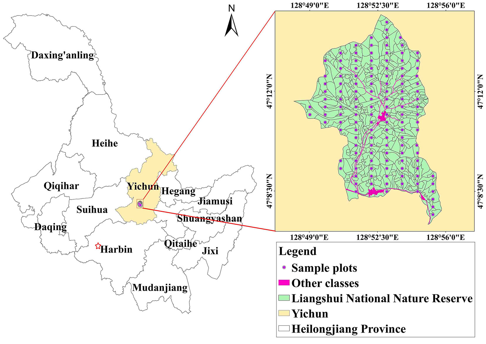
The study area of Liangshui National Nature Reserve is located in the city of Yichun, Heilongjiang Province, on the east slope of the Dalidailing branch south of the southern Xiaoxing’an Mountains and is surrounded by 6 forest farms of the Dailing Forestry Experimental Bureau. The geographical location is 47° 07′ 19″-47° 14′ 40″ N, 128° 48′ 08″-128° 55′ 45″ E (Fig. 1). The total area of the reserve is 12.133 ha, with 98% forest coverage, and the total forest volume is 1.7 million cubic meters. The study area has a temperate continental climate with an average annual temperature of -0.3 °C, and the annual average precipitation is 676.0 mm. The main forest type is mixed forest, and there are large tracts of primitive Pinus koraiensis forest and secondary birch and broad-leaved forest. The main broad-leaved tree species include Betula platyphylla, Quercus mongolica, Phellodendron amurense, Fraxinus mandshurica and Juglans mandshurica ([50]).
Fig. 1 - The study area in Yichun (northeastern China).
Survey data (variable factors)
The data were collected during an investigation for the forest resource planning and design of the Liangshui reserve in 2019, which is called the second-class survey. For the purpose of forest resource management, 31 compartments and 464 subcompartments were defined. In addition, systematic sampling was conducted every 1 km. There were 130 fixed sample plots. Each plot was round-shaped with an area of 0.06 ha. The 130 sample plots comprised 65 coniferous and broad-leaved mixed forest plots, 31 broad-leaved mixed forest plots, and 34 coniferous relatively pure forests. The main variables recorded in 130 fixed plots were geographic location (latitude and longitude), elevation (from digital elevation model - DEM, m), slope (SLOPE, deg), aspect, average age of the dominant tree species (AGE, years), canopy, average diameter at breast height of the dominant tree species (DBH, cm), total standing forest stock (TSFS, m3) and DDWV (m3). For the determination of DDWV, we recorded tree species, quantity and DBH of the DDW in each sample plot and calculated DDWV through the unitary volume table for Liangshui National Nature Reserve.
The experimental data included the fixed sample plot data and visible light (R, G and B bands) remote sensing images, which were derived from the Chinese Academy of Forestry (CAF)’s LiCHy Hyperspectra (AISA Eagle II) airborne observation system ([35]). This system is a push broom imaging system comprising a hyperspectral sensor and a data acquisition unit housed in a rugged control computer. The designed flight altitude is 1050 m, and the flight speed is approximately 160 km h-1. The image rate can be up to 160 Hz, the focal length is 18.1 mm, and the field of view (FOV) is 37.7″, with a spectral resolution of 9.6 nm and a spatial resolution of 0.52 m. In the imaging process of remote sensing images, due to changes in flight attitude, height and speed, the image pixels are distorted, offset, compressed or stretched relative to the actual position of the ground target. Therefore, we used the ENVI RPC model to perform geometric corrections for these deformations. Furthermore, for atmospheric correction, the ENVI FLAASH module was used to eliminate the absorption and scattering of electromagnetic waves from sunlight and ground objects by the atmosphere ([3], [43]). Seven kinds of visible vegetation indexes were extracted ([14], [10], [7]): the visible-band difference vegetation index (VDVI - eqn. 1), the excess green index (EXG - eqn. 2), the red:green ratio index (RGRI - eqn. 3), the excess green minus excess red index (EXGR - eqn. 4), the vegetation index (VEG - eqn. 5), the color index of vegetation (CIVE - eqn. 6), and the normalized green-red difference index (NGRDI - eqn. 7):
where R, G and B are the red band, green band and blue band, respectively, and r, g, and b are the normalized red band, green band and blue band, respectively.
Variable screening
The stepwise regression method was used to screen the seven stand factors and seven remote sensing factors. Then, to examine the models for multicollinearity, variance inflation factors (VIFs) were calculated ([33]), and variables with VIFs greater than 10 were eliminated. Descriptive statistics of the dependent variable, stand variables and remote sensing variables are shown in Tab. 1.
Tab. 1 - Descriptive statistics of the dependent variable, stand variables and remote sensing variables.
| Variables | Name | Mean | SD | Min | Q1 | Q3 | Max |
|---|---|---|---|---|---|---|---|
| Dependent variable |
Down dead wood volume (DDWV, m3) |
3.44 | 4.72 | 0.01 | 0.73 | 3.9 | 25.63 |
| Stand variables |
Elevation (DEM, m) | 401.06 | 76.22 | 270 | 344 | 430 | 638 |
| Slope (SLOPE, deg) | 8.58 | 5.21 | 1 | 6 | 10 | 36 | |
| Aspect | 5.45 | 2.31 | 1 | 4 | 7 | 9 | |
| Average age of dominant tree species (AGE, years) | 98.08 | 47.57 | 30 | 55 | 150 | 170 | |
| Canopy | 0.53 | 0.14 | 0.3 | 0.4 | 0.6 | 0.9 | |
| Average diameter at breast height od dominant tree species (DBH, cm) | 40.36 | 18.36 | 11.6 | 26 | 54 | 91 | |
| Total standing forest stock (TSFS, m³) |
14.94 | 8.17 | 0.89 | 9.4 | 18.45 | 45.97 | |
| Remote sensing variables |
Visible-band difference vegetation index (VDVI) | 0.33 | 0.03 | 0.27 | 0.31 | 0.36 | 0.41 |
| Excess green index (EXG) | 0.5 | 0.05 | 0.39 | 0.47 | 0.54 | 0.64 | |
| Red:green ratio index (RGRI) | 0.58 | 0.05 | 0.44 | 0.54 | 0.61 | 0.7 | |
| Excess green minus excess red index (EXGR) | 0.6 | 0.09 | 0.41 | 0.55 | 0.67 | 0.86 | |
| Vegetation index (VEG) | 1.95 | 0.01 | 1.67 | 1.88 | 2.02 | 2.29 | |
| Color index of vegetation (CIVE) | 18.39 | 0.02 | 18.33 | 18.38 | 18.4 | 18.44 | |
| Normalized green-red difference index (NGRDI) | 0.27 | 0.04 | 0.18 | 0.25 | 0.3 | 0.39 |
Parametric methods
OLS model
The traditional linear regression model is based on the OLS method to establish a linear relationship, as shown in eqn. 8:
where Y is the dependent variable vector, X is the independent variable vector, and β is the OLS model coefficient vector.
LMM
The LMM can be used to incorporate fixed effects and a single compartment random effect, with 31 levels ([5]), as expressed in eqn. 9:
where Y is an n×1 dependent variable vector, X is an n×p matrix of the p - 1 predictors (with the first column as 1s to estimate the intercept), n is the number of sample plots, p is the number of fixed-effect parameters, β is a p×1 vector of unknown fixed-effect parameters, Z is a known n×q design matrix for the q random effects, and γ is a q×1 vector that includes the empirical best linear unbiased predictors (EBLUPs) for the random effects. A diagonal structure was used for the covariance matrix of the compartment random-effects, while an exponential correlation structure was proposed for the residual (between-plots) covariance matrix ([49]).
GWR model
The GWR model is an extension of the traditional linear regression model and can establish local parameter estimates ([8]). The GWR model is defined as follows (eqn. 10):
where Y is the independent variable vector, (ui, vi) denotes the spatial coordinates of location i, β0(ui, vi) is the intercept, and βk(ui, vi) is the coefficient of k explanatory variables. The estimation of parameters is obtained by eqn. 11:
where W(ui, vi) is an n×n weight matrix, the off-diagonal elements of which are zero, and the diagonal elements of which are the spatial weights. GWR spatial weights can be estimated by spatial kernel functions, with Gaussian and bisquare kernel functions currently being the most common methods ([17]). The specific expression for the Gaussian function is (eqn. 12):
while for the bisquare function (eqn. 13):
where b is a non-negative decreasing function describing the functional relationship between the weight and the distance, called the bandwidth, and dij is the Euclidean distance. The model parameter estimation and prediction accuracies largely depend on the bandwidth choice. We used the corrected Akaike information criterion (AICc) to select the GWR model with the optimal bandwidth ([42]).
Nonparametric models
DNN model
With the development of computer technology, DNNs have a wide range of applications in various fields and can reliably determine the complex relationship between features ([27]). A DNN is a machine learning method for characterizing data that can simulate the neural structure of the human brain. Its core experimental steps include data processing, network model construction, network training, method selection and implementation and model generalization performance testing. In this study, the construction of DNNs relied on the Keras deep learning framework ([23]). The construction information between adjacent layers is transmitted in the form of full connections. For a hidden layer, the expression of the transfer process is shown in eqn. 14:
where l is the number of layers in the network, xl is an n×c matrix of input features, n is the batch size, c is the feature dimensions, WlT is the weight matrix, bl is the offset parameter vector, yl is the output mapping of the layer, and σ is the activation function.
In the DNN model, 4 layers of the neural network are designed to fit the complex relationships between the independent and dependent variables. Among them, the five selected variables conform to the input layer, the 2 layers in the middle are the hidden layers, and the prediction results are the output layer. The hidden layer uses a fully connected layer. The activation function is the rectified linear unit (ReLU) function, which is computationally efficient, has good sparsity and does not require unsupervised pretraining. The parameter initialization strategy enables the neural network model to learn useful information during the training process. However, the neural network model is prone to fall into local optima and is easily overfit because the initial model is complex and the amount of noise in the training set is too large. It is necessary to use the dropout algorithm to discard neurons in the hidden layer with a certain probability in the iterative training process, but their weights will be retained. The network participates in the next training iteration, and the weights are updated, which is equivalent to using multiple models to train the same dataset. Finally, the weights are assigned to the neurons to optimize the network structure.
GWDNN model
DNNs rarely consider the spatial weight problem independently and rarely consider or directly add location coordinates into the network as variables ([9], [34]). Therefore, we proposed a GWDNN model, a two-layer DNN structure in which one layer of the neural network is used to establish the spatial weights, namely, the SWNN ([15], [47]), and the other layer is used to estimate a parameter α for each variable. The theoretical structure is as follows (eqn. 15):
where w(ui, vi) is a 6×6 diagonal matrix representing the geographical weights for observation i (eqn. 16), and α is the intermediate output layer parameter predicted by the DNN (eqn. 16):
In the GWR model, spatial weighting is achieved with a function such as the Gaussian function or double square function, but its structure is simple, and it is difficult to accurately estimate nonstationarity due to the difficulty in choosing the correct kernel function for complex relationships. To address this problem, using the superior fitting ability of neural networks, Wu et al. ([47]) proposed an SWNN to construct the nonstationary weight matrix and calculated the kernel weights as the weights of a complex problem. According to this approach, the kernel weights of point i are computed as follows (eqn. 17):
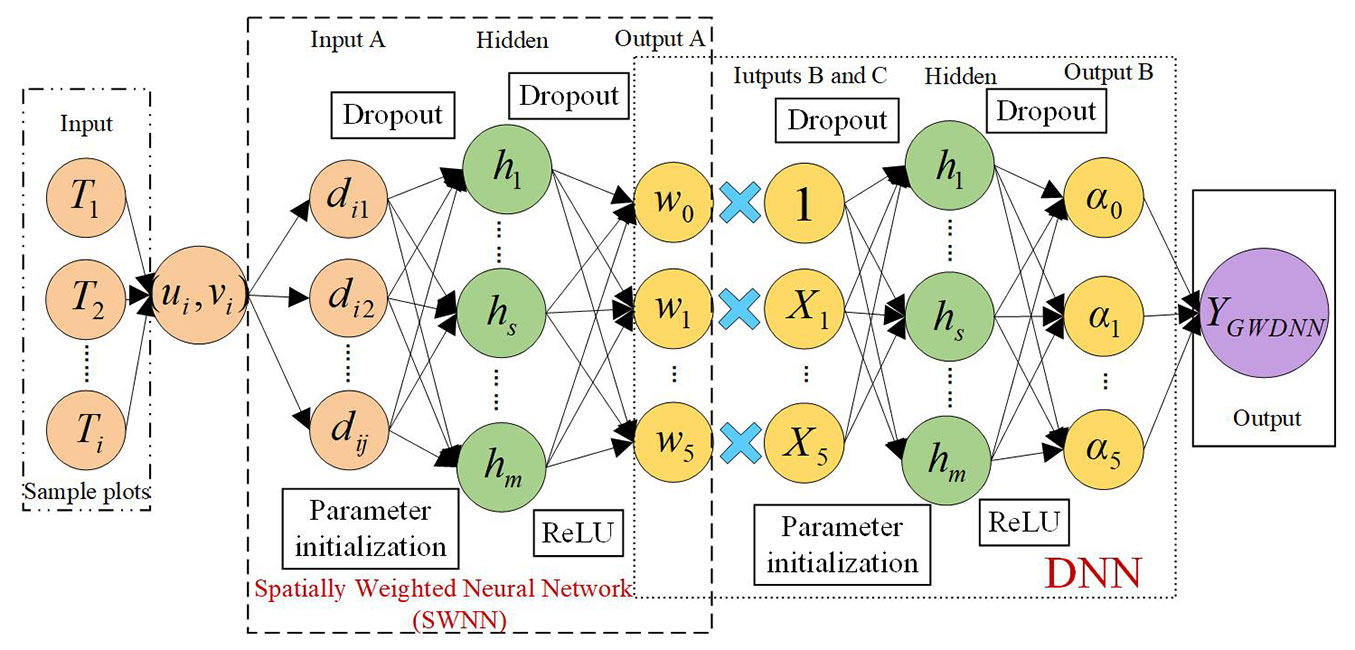
where [di1, di2, …, dij] are the distances from point i to all the samples. Consequently, the definition of the GWDNN model can be illustrated as shown in Fig. 2. The entire GWDNN contains three steps: (1) predicting the spatial weights through the coordinates (SWNN); (2) predicting the parameter α by using the DNN in OLS form; and (3) obtaining the predicted values by multiplying the independent variable, the estimated spatial weights and the parameter α.
Fig. 2 - The proposed GWDNN model for point i.
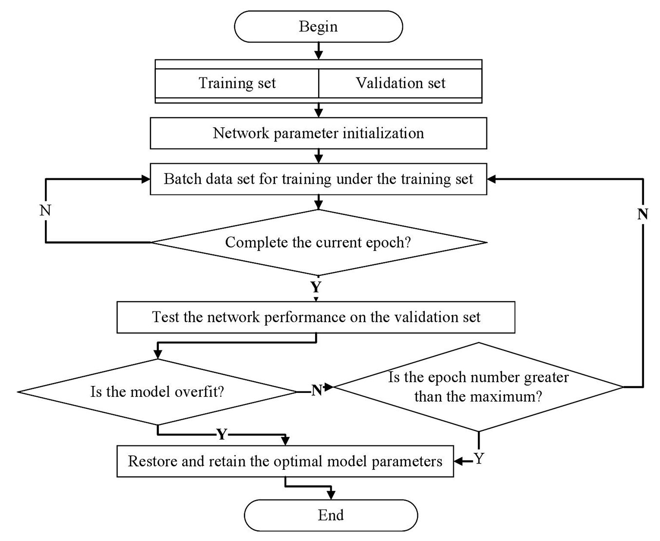
The entire training processes of the DNN and GWDNN are shown in Fig. 3. This experiment uses simple cross-validation, and the dataset is randomly divided into training sets and validation sets. During the training step, when the training process meets the early stopping condition or when the number of epochs reaches the set maximum value, the training step is completed, and the best network weights are saved. When the training process is complete, the validation set is used to estimate the predictive power of the model. The validation set does not participate in the model training process ([15]). In this paper, the MAE is used as the training loss function of the DNN and GWDNN models, and the MAE of the validation set is used as the index of overfitting. By setting the maximum number of epochs to view the trend in the MAE of the training set and the verification set, we can find the optimal model parameters under the optimal number of iterations.
Fig. 3 - Flow chart of the DNN and GWDNN training process.
The OLS model and LMM were implemented with the “nlme” library in R, and the GWR model was implemented using the “mgwr” library in Python. The DNN and GWDNN models were implemented using the “TensorFlow” and “Keras” libraries in Python.
Evaluation of DDWV models
Based on ground-truthed DDWV samples, a total of 104 samples were randomly selected from among the 130 samples from Liangshui National Nature Reserve for model training, and 26 samples were used for model verification. The R2, RMSE and MAE values were used to assess model fit and prediction ability.
Spatial effects include spatial autocorrelation and nonstationarity. Ignoring the spatial effects of a model will misleadingly reduce the significance of a test and the model’s predictive ability ([28]). To investigate the spatial autocorrelation in the model residuals, this study calculated the spatial autocorrelation index (i.e., Moran’s I) for the residuals of the five models (eqn. 18):
where xi and xj are the values of the sample locations i and j (where i ≠ j), respectively, n is the number of sample plots, bar{x} is the average of the observed values, and wij(d) is the weight estimated according to the distance between sample locations i and j.
The global Moran’s I can reveal the overall spatial autocorrelation of the study area, but if the significance of the spatial autocorrelation on each plot must be checked, the global Moran’s I must be localized ([44]); that is, the local Moran’s I must be used. Its expression is as follows (eqn. 19):
This study used Z-statistics (eqn. 20) to determine whether the spatial distribution of the model residuals was random. If the absolute value of the Z-statistic is greater than 1.96, then the independence assumption of the model residuals is contrary to the assumption of these models, and these residuals show clustering patterns. For the global and local models, we calculated the global Moran’s I separately and set Moran’s I to zero when the residual distribution was completely spatially random ([45], [50] - eqn. 20):
where (eqn. 21):
Results
Model coefficients
The dependent variable and the five standardized independent variables SLOPE, AGE, TSFS, VDVI and VEG were used to establish the five models. The regression coefficients are significant at the α level of 0.05, which shows the strong statistical significance of the five selected variables. The VIF values indicate no multicollinearity among the selected variables. Because the design of the GWDNN model is similar to that of the OLS model, we also calculated the coefficients for the GWDNN model (Tab. 2).
Tab. 2 - OLS model, LMM, GWR model and GWDNN model results.
| Model | Estimate | Intercept | SLOPE | AGE | TSFS | VDVI | VEG |
|---|---|---|---|---|---|---|---|
| OLS | Coefficient | 3.58 | 1.39 | 2.65 | -2.04 | 1.34 | -1.79 |
| SE | 0.31 | 0.33 | 0.42 | 0.41 | 0.34 | 0.37 | |
| P-value | <0.001 | <0.001 | <0.001 | <0.001 | <0.001 | <0.001 | |
| VIF | - | 1.19 | 1.81 | 1.67 | 1.23 | 1.33 | |
| LMM | Coefficient | 3.54 | 1.29 | 2.55 | -2.08 | 1.36 | -1.68 |
| SE | 0.37 | 0.39 | 0.44 | 0.41 | 0.36 | 0.39 | |
| P-value | <0.001 | 0.002 | <0.001 | <0.001 | <0.001 | <0.001 | |
| GWR | Mean_Coefficient | 3.28 | 1.16 | 2.46 | -2 | 1.29 | -1.58 |
| Min_Coefficient | 2.6 | 0.14 | 1.95 | -3.66 | 0.36 | -2.37 | |
| Median_Coefficient | 3.15 | 1.32 | 2.24 | -1.82 | 1.13 | -1.57 | |
| Max_Coefficient | 4.43 | 1.81 | 3.74 | -1.19 | 2.43 | -0.78 | |
| GWDNN | Mean_Coefficient | 2.32 | 0.05 | 1.67 | -1.08 | 0.27 | -1.05 |
| Min_Coefficient | -2.2 | -0.14 | -0.25 | -9.26 | -0.16 | -2.85 | |
| Median_Coefficient | 2.18 | 0.04 | 1 | -0.42 | 0.32 | -0.9 | |
| Max_Coefficient | 6.98 | 0.35 | 10.98 | 10.36 | 0.94 | -0.29 |
Hyperparameter analysis of the nonparametric models
The setting of the parameters in the DNN and GWDNN models is particularly important in the training process. The DNN is fully connected with a total of 4 layers. The network layer includes 1 input layer, 2 hidden layers and 1 output layer. The numbers of neurons are set to n × 5, n × 32, n × 32 and n × 1; the initial learning rate (LR) is set to 0.001; the maximum number of epoch iterations is 2000; the batch size is 10; and the dropout rate of the dropout layer is 0.5. Two branches are set in the middle of the GWDNN structure: one branch is used to find the spatial weight, and the number of features in each layer is [n × 130, n × 128, n × 128, n × 128, n × 6]; the other branch is used to find the parameters, and the number of features in each layer is [n × 6, n × 64, n × 64, n × 6], among which the independent variabels and the set 1 are used to obtain the output layer n × 1, the initial LR is set to 0.001, the maximum number of epoch iterations is 2000, the batch size is 5, and the dropout rate of the dropout layer is 0.4. The specific DNN and GWDNN hyperparameters are shown in Tab. 3.
Tab. 3 - DNN model and GWDNN model hyperparameter settings.
| Hyperparameter | DNN model |
GWDNN model |
|---|---|---|
| Input | n×5 | n×130 (A), n×6 (BC) |
| Hidden1 | n×32 | n×128, n×64 |
| Hidden2 | n×32 | n×128, n×64 |
| Hidden3 | - | n×128 |
| Output | n×1 | n×1 |
| LR | 0.001 | 0.001 |
| Epoch maximum |
2000 | 2000 |
| Dropout | 0.5 | 0.4 |
| Batchsize | 10 | 5 |
| Epoch stop | 1175 | 792 |
Model evaluation
Tab. 4presents the training sets and validation sets of the 5 models for fitting and predicting DDWV. For both the training set and the validation set, the GWDNN model is the best performing model, and the OLS model is the worst. The evaluation index results for the LMM and GWR model are similar. However, the fitting accuracy of the LMM is slightly higher than that of the GWR model, whereas prediction accuracy exhibits the opposite pattern. The nonparametric models perform much better than the parametric models in fitting and prediction accuracy. Compared with that of the GWR model, the RMSE of the DNN model was decreased by 28% and 41%, and that of the GWDNN model was decreased by 61% and 45%.
Tab. 4 - Simple cross-validation model evaluation of the training set and validation set.
| Models | Training set | Validation set | ||||
|---|---|---|---|---|---|---|
| R2 | RMSE | MAE | R2 | RMSE | MAE | |
| OLS | 0.57 | 3.08 | 2.26 | 0.43 | 3.60 | 2.57 |
| LMM | 0.71 | 2.52 | 1.81 | 0.46 | 3.51 | 2.69 |
| GWR | 0.69 | 2.59 | 1.91 | 0.52 | 3.31 | 2.34 |
| DNN | 0.84 | 1.86 | 1.33 | 0.83 | 1.96 | 1.40 |
| GWDNN | 0.95 | 1.05 | 0.77 | 0.85 | 1.82 | 1.39 |
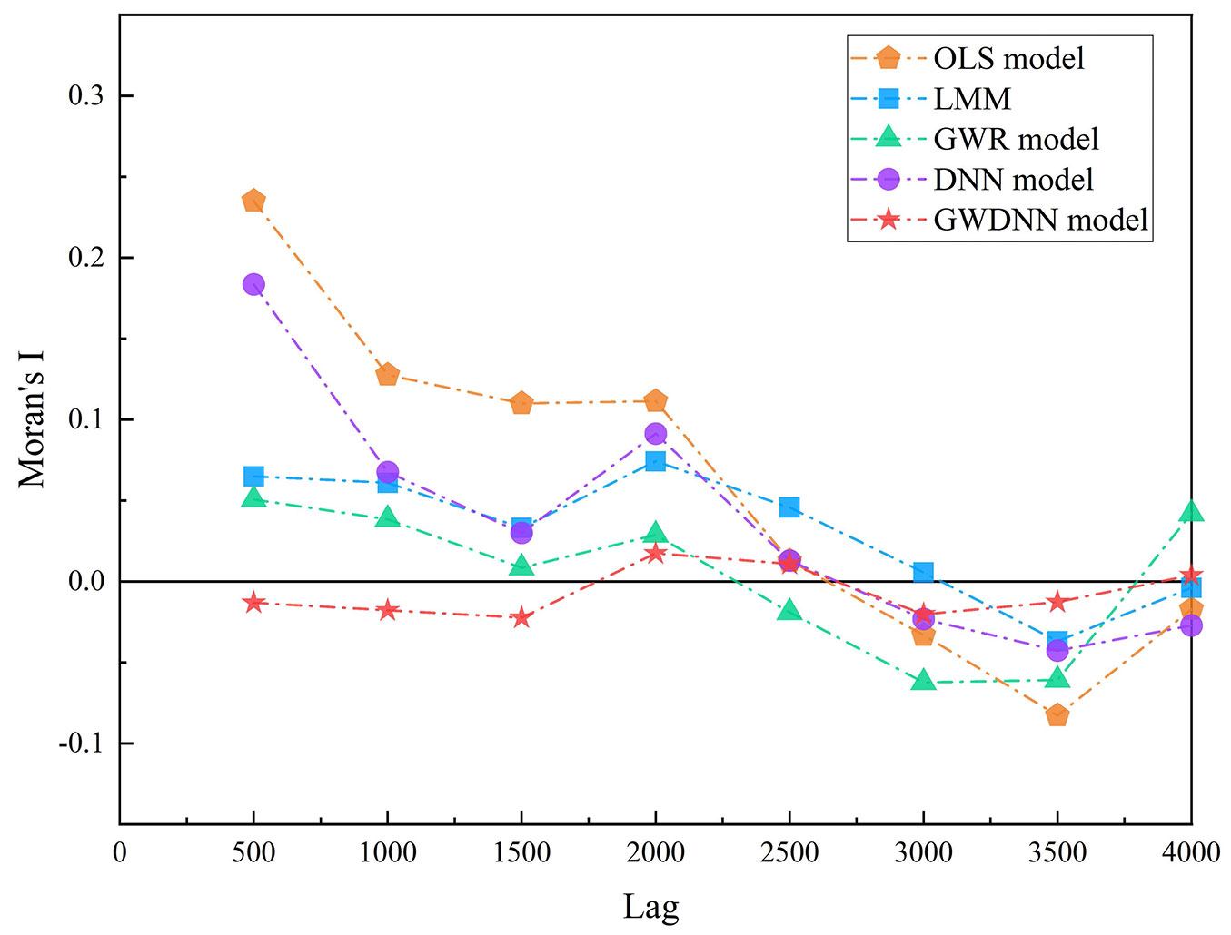
Tab. 5shows the spatial correlation of the model residuals (Moran’s I and Z-statistic values). The results show that the residuals of the OLS model have significant spatial autocorrelation. The residuals of the LMM and the GWR, DNN and GWDNN models have nonsignificant spatial autocorrelation. In general, the Z-statistics can be compared among the models. The models eliminated spatial autocorrelation in the following order: GWDNN > GWR > LMM > DNN > OLS. The spatial correlation of the residuals of the DNN, which does not consider spatial effects, is high. When considering the spatial weights in the GWDNN model, the spatial autocorrelation is eliminated very well. To compare the spatial relationship of the residuals among the models, residual spatial correlation diagrams of the five models were constructed at 500 m intervals (Fig. 4). Moran’s I is relatively stable across step lengths for the GWDNN model and close to zero at all step lengths in the other models. This finding shows that the GWDNN model has a good ability to maintain spatial stability.
Tab. 5 - Global Moran’s I values of the residuals of the five models.
| Model | Moran’s I | Z-statistic |
|---|---|---|
| OLS | 0.24 | 2.29 |
| LMM | 0.06 | 0.8 |
| GWR | 0.05 | 0.64 |
| DNN | 0.17 | 1.95 |
| GWDNN | -0.01 | -0.06 |
Fig. 4 - The spatial correlation between residuals for the five models.
Mapping of the spatial distribution of DDWV
With reference to the ground-truthed DDWV data, the results of the five different models were compared. According to the general kriging interpolation in ArcGIS® v. 10.4 (ESRI, West Redlands, CA, USA) geostatistical analysis, the spatial interpolation process is similar to the weighted moving average ([25]). The cartography can be visualized by using the symbolic representation principle ([9]) to more directly depict the spatial variation and details of the DDWV in Liangshui National Nature Reserve (Fig. 5).
Fig. 5 - Spatial distribution of (a) the ground-truth DDWV (down dead wood volume, m3), and (b-f) the results of the five predicting models.
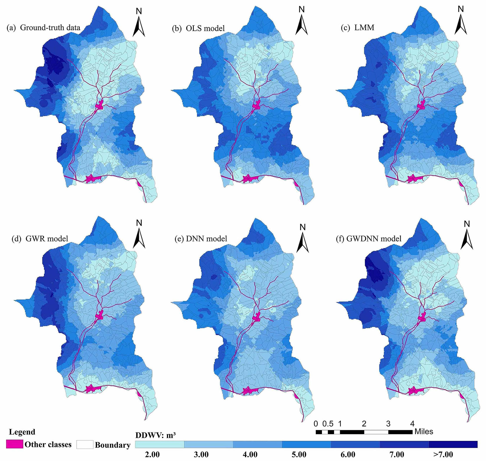
The overall trend in the measured DDWV and the spatial distributions from the five models are consistent. The DDWV values ranged from 2.00 to 7.00 m3. To facilitate comparison, the values were divided into seven levels by equal intervals of 1 m3 (Fig. 5). The maps show the various spatial distributions of DDWV. All six maps show that the western part of the Liangshui reserve is a high DDWV region, with values greater than 7 m3, while low DDWV regions are located near the river and road in the middle and western parts of Liangshui National Nature Reserve, with values ranging from 0.00 to 2.00 m3. The DNN model predicted poor levels in this region. The map resulting from the GWDNN model exhibited more explicit spatial variations than the other maps.
On the whole, the GWDNN model results are closer to the measured data and can describe the spatial distribution of DDWV in more detail than the other model results. Such maps can guide resource allocation for forest management. The forest DDWV mapping results of these models were insufficient for evaluation in this study, as we were limited by sample size. Future verification work should be conducted; conventionally, such verification work is performed by using independent sample sets or acknowledged high-accuracy results such as airborne data, especially unmanned aerial vehicle LiDAR data ([9], [29]).
Discussion
Stand and remote sensing predictors
Currently, in the already existing models for mortality and CWD distribution, the predictors are usually stand factors, which have been confirmed to have great potential in previous studies ([41], [50], [4]). In other forest models, multispectral characteristics, texture characteristics and vegetation index are used as predictive variables, and the near infrared, which is more sensitive than other wavelengths, is used as the band of vegetation to compute the normalized difference vegetation index (NDVI) and the enhanced vegetation index (EVI - [13]). These remote sensing factors have pioneering significance in machine learning and local regression estimation. However, because there is only one visible light band and no near-infrared band in many data, scholars have studied visible light vegetation indexes, such as the VDVI, in place of the NDVI. The present study represents the first time in which the visible vegetation index and terrain and stand factors have been used to establish a DDWV model. The results show that visible remote sensing factors can be used to extract important information for DDWV estimation.
The model coefficients of traditional parametric models include a substantial amount of information (Tab. 2). The regression coefficients of the five selected variables are significant at an α level of 0.05. Among them, the model coefficients of SLOPE, AGE and VDVI are positive, indicating positive correlations with the dependent variable (DDWV). Thus, for example, when holding the other predictor variables constant, the steeper the slope, the higher the DDWV. The coefficients for TSFS and VEG are negative, indicating negative correlations with the dependent variable (DDWV). This result indicates that DDWV in the study area is more strongly associated with larger trees, commonly older trees, with low TSFS ([50]). Because the GWDNN model was constructed in the form of an OLS model, statistics were calculated for the coefficients of the GWDNN model. In the GWDNN model, the coefficients of VEG were negative values, while the coefficients of the other variables exhibited positive and negative values. In other words, the variation in the GWDNN coefficients was greater than that of the GWR coefficients, which might explain the significant increases in fitting performance and prediction performance achieved with the GWDNN model.
Model comparison
The fitting accuracy and prediction accuracy were compared among the five models based on the R2, RMSE, MAE, Moran’s I, Z-statistic, combined accuracy, and residual spatial autocorrelation results, and revealed that the GWDNN model is the best. In many studies, machine learning has been proven to be significantly superior to the GWR model and the LMM ([6], [9]). However, there are many differences between the LMM and GWR model. For example, Quirós-Segovia et al. ([39]) discovered that the quality of the height-diameter models of GWR and LMM regressions were comparable. Wei et al. ([46]) studied the spatial distribution of PM2.5 and found that the LMM was better than the GWR model; however, the GWR model has been shown to perform better than the LMM in many other studies ([30], [49]). For the GWDNN model, a multi-layer DNN was constructed to consider the influence of the spatial weights on the model, which improved the spatial influence after only considering the geographic position coordinates as variables previously.
The potential of the different models was demonstrated during the modeling process: establishment of the OLS model is simple and fast, and the correlations between different variables can be found intuitively. The GWR model considers the model results under different bandwidths. The advantage of the GWR model over the LMM is the possibility of determining the spatial location of every parameter without additional measurements ([49]). The DNN model has strong fitting and verification ability but cannot eliminate the spatial autocorrelation. The GWDNN model combines the SWNN and DNN and achieves accurate deconstruction and efficient calculation of spatial nonstationarity. The GWDNN model achieves excellent performance. In terms of predicting the spatial distribution of DDWV, the GWDNN model results are the closest to the ground-truthed distribution. In addition to offering statistical graphics and GIS mapping capabilities, the GWDNN model can intuitively provide key information on the distribution of DDWV, which is of great significance for forest decision-making and management planning.
Conclusion
DDWV was predicted by using parametric and nonparametric models of stand and remote sensing factors. The nonparametric models were found to be far superior to the parametric models in terms of fitting and verification accuracy, and the Moran I and Z-statistic values of the DNN model were lower than those of the LMM and the GWR model in terms of the stability of the model residual space. However, by changing the network structure to consider the spatial weights, the GWDNN model showed greater advantages in fitting and verification, and produced ideal residuals by verifying the spatial autocorrelation. Through the application of GIS technology in the study area, clear spatial distribution information was obtained; thus, this method enables very good assessment of the damage caused by natural disasters and can provide key information on forest resources for decision-making and management plans and be used to prevent and reduce the disturbance due to natural disasters and losses.
In summary, the results of this study suggest that the feasibility of the GWDNN model as a spatial model should be further investigated and promoted in the future. DNNs are popular algorithms that can mine data better than other networks. However, due to the lack of a clear connection between network parameters and approximate mathematical functions, DNNs are often called “black boxes”.
Acknowledgments
Y.S. and W.J. designed the research; Y.S. Y.C. and K.X. performed the experiments; Y.S. and Z.A. conducted the analysis and wrote the paper. All authors reviewed the manuscript.
This research was funded by the National Natural Science Foundation of China, grant no. 31870622, and the Special Fund Project for Basic Research in Central Universities, grant no. 2572019CP08. The authors are grateful to the First Investigation and Planning Institute of Forestry and Grassland in Heilongjiang Province and Liangshui National Nature Reserve for providing the second-class survey data in 2019.
References
Online | Gscholar
Gscholar
Gscholar
Authors’ Info
Authors’ Affiliation
Ziqi Ao
Weiwei Jia 0000-0001-7318-8997
Ying Chen
School of Forestry, Northeast Forestry University, Harbin 150040 (China)
CosmosVision Robot of Anhui Zhong’an Chuanggu Technology Park, Hefei 230000 (China)
Corresponding author
Paper Info
Citation
Sun Y, Ao Z, Jia W, Chen Y, Xu K (2021). A geographically weighted deep neural network model for research on the spatial distribution of the down dead wood volume in Liangshui National Nature Reserve (China). iForest 14: 353-361. - doi: 10.3832/ifor3705-014
Academic Editor
Maurizio Marchi
Paper history
Received: Nov 27, 2020
Accepted: Jun 03, 2021
First online: Jul 27, 2021
Publication Date: Aug 31, 2021
Publication Time: 1.80 months
Copyright Information
© SISEF - The Italian Society of Silviculture and Forest Ecology 2021
Open Access
This article is distributed under the terms of the Creative Commons Attribution-Non Commercial 4.0 International (https://creativecommons.org/licenses/by-nc/4.0/), which permits unrestricted use, distribution, and reproduction in any medium, provided you give appropriate credit to the original author(s) and the source, provide a link to the Creative Commons license, and indicate if changes were made.

Web Metrics
Breakdown by View Type
Article Usage
Total Article Views: 33815
(from publication date up to now)
Breakdown by View Type
HTML Page Views: 28597
Abstract Page Views: 2276
PDF Downloads: 2460
Citation/Reference Downloads: 5
XML Downloads: 477
Web Metrics
Days since publication: 1448
Overall contacts: 33815
Avg. contacts per week: 163.47
Article Citations
Article citations are based on data periodically collected from the Clarivate Web of Science web site
(last update: Mar 2025)
Total number of cites (since 2021): 12
Average cites per year: 2.40
Publication Metrics
by Dimensions ©
Articles citing this article
List of the papers citing this article based on CrossRef Cited-by.
Related Contents
iForest Similar Articles
Research Articles
Analyzing regression models and multi-layer artificial neural network models for estimating taper and tree volume in Crimean pine forests
vol. 17, pp. 36-44 (online: 28 February 2024)
Research Articles
Identification of wood from the Amazon by characteristics of Haralick and Neural Network: image segmentation and polishing of the surface
vol. 15, pp. 234-239 (online: 14 July 2022)
Research Articles
Bayesian geographically weighted regression and its application for local modeling of relationships between tree variables
vol. 11, pp. 542-552 (online: 01 September 2018)
Research Articles
The use of tree crown variables in over-bark diameter and volume prediction models
vol. 7, pp. 132-139 (online: 13 January 2014)
Research Articles
Estimating biomass of mixed and uneven-aged forests using spectral data and a hybrid model combining regression trees and linear models
vol. 9, pp. 226-234 (online: 21 September 2015)
Research Articles
Nonlinear mixed model approaches to estimating merchantable bole volume for Pinus occidentalis
vol. 5, pp. 247-254 (online: 24 October 2012)
Research Articles
Use of LIDAR-based digital terrain model and single tree segmentation data for optimal forest skid trail network
vol. 8, pp. 661-667 (online: 22 December 2014)
Research Articles
Total tree height predictions via parametric and artificial neural network modeling approaches
vol. 15, pp. 95-105 (online: 21 March 2022)
Review Papers
Remote sensing-supported vegetation parameters for regional climate models: a brief review
vol. 3, pp. 98-101 (online: 15 July 2010)
Research Articles
Assessing the availability of forest biomass for bioenergy by publicly available satellite imagery
vol. 11, pp. 459-468 (online: 02 July 2018)
iForest Database Search
Search By Author
Search By Keyword
Google Scholar Search
Citing Articles
Search By Author
Search By Keywords


