Daily prediction modeling of forest fire ignition using meteorological drought indices in the Mexican highlands
iForest - Biogeosciences and Forestry, Volume 14, Issue 5, Pages 437-446 (2021)
doi: https://doi.org/10.3832/ifor3623-014
Published: Sep 28, 2021 - Copyright © 2021 SISEF
Research Articles
Abstract
We analyzed the behavior of forest fires for daily prediction purposes in one of the regions with the highest fire incidence in Mexico. The main objective was to build logistic regression models (LRMs) for daily prediction of forest fire ignition based on meteorological drought indices. We built 252 LRMs for seven types of vegetation cover of greater representativeness and interest for the study area. Three dynamic variables were considered to estimate daily dryness in combustible fuels based on the effective drought index and the standardized precipitation-evapotranspiration index. Additionally, two weather data sources were included in drought indices: conventional weather stations (CWS) and automatic weather stations (AWS). Prediction efficiency assessment for LRMs was done through the relative operating characteristic (ROC) and model precision efficiency (MPE). The results show that LRMs using data from CWS performed relatively better than those based on data from AWS, as the former data sources have higher spatial density and thus generate predictions with higher accuracy (ROC ≥ 0.700, MPE ≥ 0.934). For both data sources, the use of standardized precipitation-evapotranspiration index as a fuel dryness estimator is recommended, as it reflects an atmospheric moisture balance between precipitation and reference evapotranspiration (ROC ≥ 0.734, MPE = 1). Such predictive models can be used as inputs in early warning systems for forest fire prevention or mitigation.
Keywords
Logistic Regression, Effective Drought Index, Standardized Precipitation-Evapotranspiration Index, Conventional Weather Stations, Automatic Weather Stations
Introduction
Wildfires are natural agents that regulate several ecosystems worldwide. These phenomena respond to climate characteristics and vegetation resistance to ignition during periods of drought. Some benefits of fire in ecosystems include the reduction of plant competition for water and soil resources, sanitation and disease control of vegetation, the release of nutrients and seed germination of several species ([9]).
Several factors influence the ignition and spread of fire in a wildfire: (i) meteorological aspects ([31]), such as temperature ([33]), wind speed and direction ([6]), solar radiation, and precipitation ([44]); (ii) geographical aspects ([31]), such as slope ([33]) and orientation of slopes that may receive further insolation ([35]); (iii) anthropogenic aspects, such as the distance to communication routes, agricultural burning, campfires of walkers, cigarette butts, and intentional actions ([9], [10], [13]). According to the National Forestry Commission of Mexico ([9]), the conditions influencing fire ignition and spread can be grouped as: (i) permanent conditions, such as fuel loading, vegetation coverage, slope, and orientation of slopes; (ii) dynamic conditions, such as temperature, wind speed and direction, solar radiation, and precipitation. Further, Guo et al. ([15]) group the causes of fires as regional (e.g., climate) and local (e.g., vegetation, topography, and human activities).
Previous studies found that logistic regression models (LRMs) for fire ignition prediction have become relevant due to the relative simplicity of their construction. For example, research in Australia was conducted based on patterns and driving factors of fire occurrence ([46]). In Mexico, it has been shown that wildfires are related to human influence and conditions ([8]). In Portugal, researchers associated the magnitude of fires with vegetation, land use, climate factors, and human actions ([12]); whereas in China, driving forces of the occurrence of fires were assessed as regional and local factors ([15]).
According to Vicente-Serrano et al. ([41]), the use of meteorological drought indices to estimate the dryness of fuels was adopted because no physical variables can accurately quantify drought. Drought and dry fuels are highly correlated phenomena that can be helpful in fire prediction ([17]). The meteorological drought indices used in this study were the effective drought index (EDI) and the standardized precipitation-evapotranspiration index (SPEI). The use of these indices is due to their popularity and effectiveness in modeling the drought phenomenon during the last decade ([17]). Some studies have used drought indices such as SPEI to identify the occurrence of fires ([37], McEvoy et al. ([26]), whereas Hadisuwito & Hassan ([17]) analyzed SPEI and EDI as fire-compatible indices. In this study, we used the EDI index which employs a precipitation reduction function to estimate soil moisture conditions ([7]).
The main goal of this study was to develop LRMs for daily prediction of forest fire ignition in Mexican highlands using meteorological drought indices. The specific objectives were: (i) estimating EDI and SPEI drought indices from conventional weather stations (CWS) and automatic weather stations (AWS) data sources; (ii) calculating three explanatory variables on a daily basis from EDI and SPEI indices as an estimate of the dryness of fuels prone to fire; (iii) generating LRMs for every month and for each of the main types of vegetation in the study area; (iv) assessing the level of certainty of each LRM in predicting fire occurrence.
Materials and methods
Study area
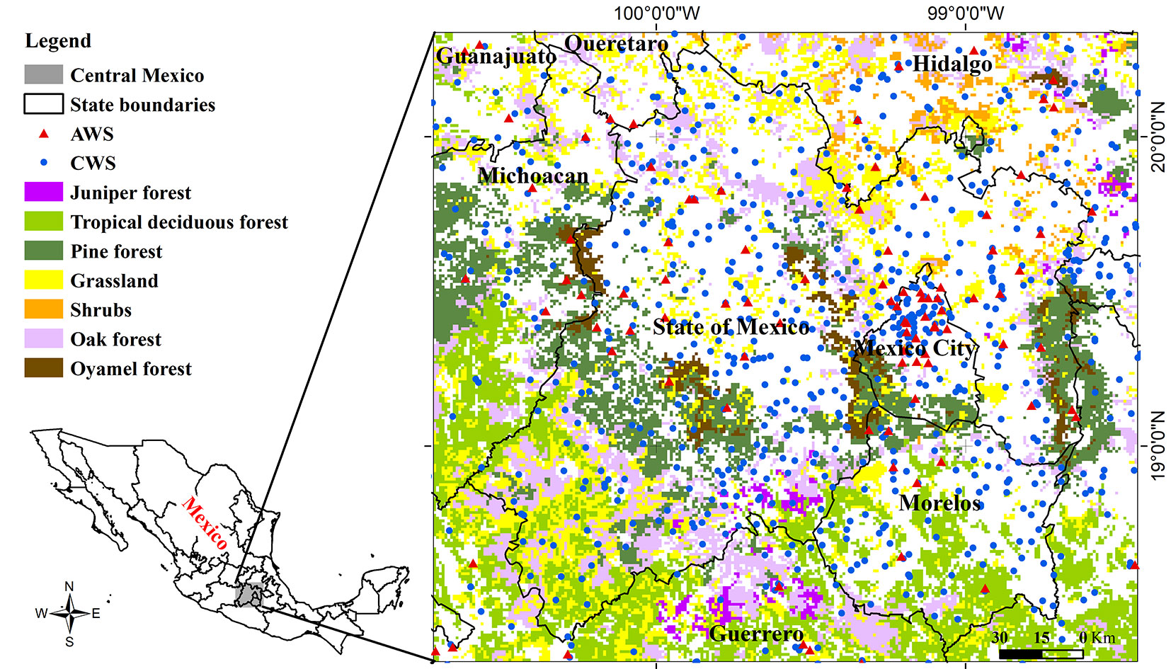
The study area is to the central region of the Mexican plateau (18° 18′ - 20° 20′ N, 98° 27′ - 100° 43′ W - Fig. 1) covering an area of 53.962 km2 with more than 32 million inhabitants. The altitude in the region ranges between 226 and 5400 meters a.s.l. Four types of climate can be identified: (i) temperate sub-humid with annual rainfall between 600 and 1000 mm; (ii) warm sub-humid with annual rainfall between 1000 and 2000 mm; (iii) dry with annual rainfall from 300 to 600 mm; and (iv) cold weather in the highlands of volcanoes. About 52% of the territory is covered by agricultural and urban areas ([21]), while the rest has tropical deciduous forest (26.2%), grassland (24.2%), oak forest (21%), pine forest (19.8%), oyamel forest (3.9%), shrubs (3.1%), and juniper forest (1.8%).
Fig. 1 - Map of vegetation types and localization of the weather stations (CWS: blue circles; AWS: red triangles) in the Mexican highlands.
Datasets
Weather data
Two weather data sources were considered for the calculation of drought indices: conventional weather stations (CWS) and automatic weather stations (AWS). Among the most significant differences between CWSs and AWSs are the observation and data registration processes. In a CWS, atmospheric variables are measured once a day and recorded by an observer, whereas in AWSs, the logs are automatic and recorded between 48 and 144 times a day ([45]). Globally, CWSs have a denser spatial network than AWSs in Mexico, though AWSs have more timely coverage of data than CWSs. Daily precipitation data and maximum and minimum temperatures for the training period (2006-2014) were obtained from 748 CWS stations. Because the AWS network in Mexico has been established recently, we considered meteorological data from 124 AWS stations in the training period (2012-2014), namely daily precipitation and maximum and minimum temperatures (Fig. 1). For both CWSs and AWSs, model validation was performed on data collected in 2015.
Forest fires
According to images from NASA’s MODIS sensor, in the period from 2003 to 2016, 1.300.000 fires occurred worldwide ([3]), of which 8.6% in Mexico, and 23.4% of these occurred in the Mexican highlands ([10]). The Forest Protector of the State of Mexico (PROBOSQUE) is a local institution that collects and provides daily fire records in the region. The date, start time, duration, cause, burned surface, and geographic coordinates (centroid of the burned area) of the fire event are recorded in this dataset ([30]). In this study, we used daily data of 2320 fires from 2006 to 2015.
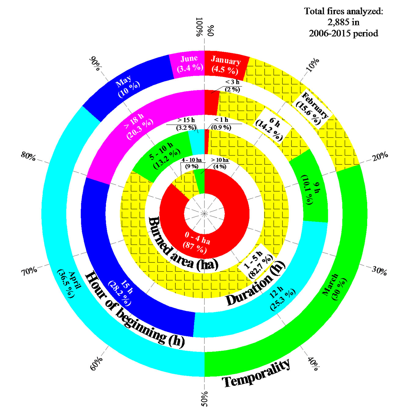
The outermost ring in Fig. 2shows that the fire season extends over the first months of the year, especially March (30% of the total fire events in the area) and April (36.5%). Also, wildfires predominantly start between 1:00 and 3:00 p.m. (53.5% of events), i.e., the hottest and driest hours due to sunstroke. Additionally, the mean duration of the fires is between one and five hours (82.7% of events), and the burned area is less than 4 ha in 87% of fire events (Fig. 2).
Fig. 2 - Forest fire characteristics in Mexican highlands (source: [30]). Overall, 2885 fires were analyzed in the period 2006-2015. The burned area (innermost ring) is expressed in hectares, duration (second concentric ring) in hours, hour of beginning (third concentric ring) in hours, and the temporality (outermost ring) is the frequency of monthly occurrence of fires. The percentage of fire occurrence is in parentheses.
Logistic regression model
A logistic regression model (LRM) was used to predict the daily occurrence of fire ignition. An LRM is developed using a dependent variable, which is defined as the response observed by the combined influence of other independent variables ([20]). In the logistic regression model the dependent variable has two possible values: “1” for the occurrence of the event and “0” (zero) for the opposite. The model is implemented using eqn. 1 and eqn. 2:
where β0 is the regression constant (intercept) and βk is the weight of the k-th independent variable xk. The result of the function P estimates the probability of occurrence of the event, i.e., in this study the probability of fire occurrence.
Dependent variable
Seven representative types of vegetation cover with a high frequency of fires were identified in the study region: pine forests, oak forests, oyamel forests, juniper forests, tropical deciduous forests, grassland, and shrubland (Fig. 1). Daily fire maps were produced for each vegetation type by overlaying the map of each type of vegetation with satellite images of fire occurrence: the dependent variable took the value “1” for pixels affected by the wildfire, and “0” otherwise.
Static and semi-static independent variables
The independent variables were selected according to the results of Vilchis-Francés et al. ([43]), who used principal component analysis (PCA) to obtain the best explanatory fire variables, finding that fuels dryness, maximum wind, distance to roads, orientation and slope of the hillsides explained more than 89% of the total observed variance in fire occurrence ([43]).
The four variables mentioned above were used in this study and were classified as static (track distance, slope, and slope orientation) and semi-static (maximum wind speed), thus generating the following:
- Distance to roads: it reflects the distance from communication routes such as train tracks, roads, terraces, and gaps, as well as infrastructure associated with roads such as tunnels, bridges, and collection places ([21]).
- Slopes and hillside orientation: a digital elevation model (DEM) was used to calculate the slope and orientation of the hillsides.
- Maximum wind speed: although this variable is very dynamic, it was considered a semi-static variable because CWS stations in Mexico do not have anemometers. It was generated with data available from AWS stations from 2012 to 2015, and used as a monthly average for CWS and AWS models in their corresponding periods.
Dynamic independent variables
Daily data from CWS and AWS sources were used to build EDI and SPEI meteorological drought indices. The following fuel dryness variables were defined: (i) CN-DEP (consecutive days of negative deviation for effective precipitation) from the EDI Index; and (ii) CN-SPEI (consecutive days of negative SPEI value).
CN-DEP calculation
The effective drought index (EDI) defines the effective precipitation EPi as the reduction of daily precipitation of previous m days ([7]). Precipitation from previous days is added to total water availability as a form of average precipitation (eqn. 3):
where EPi is the effective daily precipitation in millimeters, pm is the precipitation of the m previous days in millimeters, and i is the duration of the sum of the previous days. In this work, m was set to 15 because this value represents the total water stored in the soil for short periods, as suggested by Byun & Wilhite ([7]).
The effective precipitation deviation (DEP) was calculated as follows (eqn. 4):
where DEPi is the deviation of the effective precipitation EPi from the effective average precipitation (MEPi) of previous years.
Finally, the CN-DEP was obtained by determining the duration of each period with moisture deficiency. This index was calculated based on the consecutive number of days showing negative DEPi values (Tab. 1).
Tab. 1 - Example of the estimation of CN-DEP or CN-SPEI by counting consecutive days with moisture deficit. (ISPEI/DEP): series with variable change (1: SPEI or DEP < 0; 0: SPEI or DEP ≥ 0); (ΣDSPEI/DEP): sum of consecutive days with a moisture deficit (CN-DEP or CN-SPEI with value 1). At day 6, the CN-DEP or CN-SPEI value is 4 (third column) because the previous days of the CN-DEP or CN-SPEI value are 1 (second column), and the accumulated value is 4. The 7th day has a CN-DEP or CN-SPEI value of 0 (third column) because the CN-DEP or CN-SPEI value is 0.
| Day | ISPEI/DEP | ΣDSPEI/DEP |
|---|---|---|
| 1 | 0 | 0 |
| 2 | 0 | 0 |
| 3 | 1 | 1 |
| 4 | 1 | 2 |
| 5 | 1 | 3 |
| 6 | 1 | 4 |
| 7 | 0 | 0 |
| 8 | 0 | 0 |
| 9 | 1 | 1 |
| .... | .... | .... |
SPEI calculation
The SPEI represents a standardized atmospheric moisture balance and reflects the deviation of moisture conditions from dryness. The difference D between precipitation availability and demand for reference evapotranspiration ([40]) is calculated as (eqn. 5):
where Di is the moisture balance in the i-th day, pi is the precipitation, PETi is the reference evapotranspiration, calculated according to Hargreaves & Samani ([18]). Finally, SPEI was obtained as follows (eqn. 6, eqn. 7):
where p is the probability of surplus for D, and C0 = 2.515517, C1 = 0.802853, C2 = 0.010328, d1 = 1.432788, d2 = 0.189269, d3 = 0.001308 are constant values ([40]).
CN-SPEI calculation
This index is based on the EDI method proposed by Byun & Wilhite ([7]) for SPEI estimation, adapted as follows: (i) SPEI ([40]) is obtained at daily scale based on eqn. 5, eqn. 6, and eqn. 7; (ii) SPEI results are reclassified as “1” when SPEI < 0 and “0” when SPEI ≥ 0; this new binary variable was named consecutive days of negative index SPEI (CN-SPEI); (iii) the consecutive CN-SPEI values equal to 1 ([7]) are counted, where each positive value stops the sum and resets the count to 0 (Tab. 1); this sum was called CN-SPEI and is expressed in days.
Construction of LRM
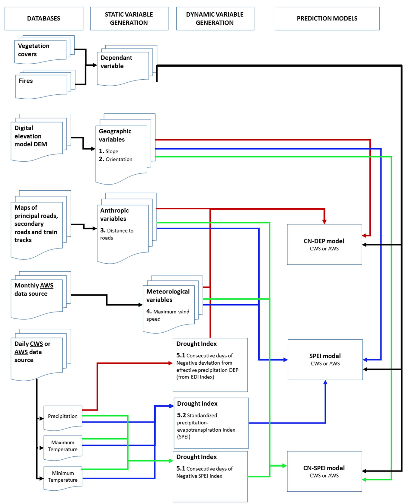
Building LRM starts with integrating CWS and AWS data sources to calculate dependent and dynamic variables. These models were called CN-DEP, SPEI, and CN-SPEI, corresponding to the dynamic variables of fuel dryness (Fig. 3). Six LRMs were developed with the weather data source and the fuel dryness variables (CWS-CN-DEP, CWS-SPEI, CWS-CN-SPEI, AWS-CN-DEP, AWS-SPEI, and AWS-CN-SPEI). Each LRM was built for each month of the fire season (January to June) and for each of the types of vegetation described above. All variables were standardized in raster format with a pixel resolution of 1 km2. Given that the burned area of most fires is less than 4 ha (0.04 km2), it is assumed that a single pixel in the vegetation cover is thoroughly burned, which does not always happen. However, the distance between daily fires was checked, and none were within 1 km of each other.
Fig. 3 - General flow chart of the construction of forest fire prediction daily models using drought indices.
Standardization of units and magnitudes of independent variables
The variables were normalized with values between 0 and 1 to avoid assigning greater weights to variables of greater magnitude. The value 1 was assigned to pixels having magnitudes of each variable that most affect fire ignition in the study area, and 0 to the rest (Tab. 2). For example, we considered the danger of fire ignition to be greater within a distance of 200 m on each side of the roads, due to possible campfires, throwing of cigars ([8]) or sparkles from the friction of train wheels on tracks. Besides, agricultural areas are usually close to secondary roads where fires can quickly get out of control ([10]). Therefore, the value 1 was assigned to pixels at distances < 200 m from roads, train tracks, or crop fields, and 0 for further distances.
Tab. 2 - Magnitudes normalization of the explanatory variables included in the logistic regression models (LRMs) and their units.
| Variable | Explanatory variable | Units | Magnitude (M) |
Scale (in LRM) |
|---|---|---|---|---|
| Static | Distance to roads | m | 0 ≤ M ≤ 200 | 1 |
| M > 200 | [1, 0] | |||
| Slope | deg | 0 ≤ M ≤ 59.2 | [0, 1] | |
| Orientation (Aspect) | deg | 0 ≤ M ≤ 45 | 0 | |
| 45 < M ≤ 135 | [0, 1] | |||
| 135 < M ≤ 225 | 1 | |||
| 225 < M ≤ 315 | [1, 0] | |||
| 315 < M ≤ 359.9 | 0 | |||
| Semi-Static | Wind speed | m s-1 | 0 ≤ M ≤ 6.22 | [0, 1] |
| Dynamic (drought index) | (i) CN-DEP | day | 0 ≤ M ≤ 60 | [0, 1] |
| M > 60 | 1 | |||
| (ii) SPEI | - | -5 ≤ M < 0 | [1, 0] | |
| M ≥ 0 | 0 | |||
| (iii) CN-SPEI | day | 0 ≤ M ≤ 60 | [0, 1] | |
| M > 60 | 1 |
The slope of hills affects fires when they are more pronounced, as fire spreads faster in conjunction with wind speed ([44]). The value 1 was assigned to pixels with the maximum slope in the study area (52.9°), whereas 0 was assigned to pixels showing minimum slope. Hillside orientation has a more significant impact on fire when exposed to increased radiation, as fuels such as leaves and branches on the ground are heated and dried ([44]). In the study area, pixels of hillsides with south, southeast, and southwest orientation (135° to 225°) took the value of 1, while the value 0 was assigned to orientations northeast (45° to 135°) and northwest (225° to 315°). The wind favors fire the higher its speed ([6]). Thus, value 1 was assigned to pixels showing the maximum wind speed recorded in the region (6.22 m s-1), and 0 to minimum values (close to 0).
Regarding dry fuels, we assigned a value of 1 to pixels subject to 60 consecutive days with moisture deficit (CN-DEP and CN-SPEI). Indeed, according to Turco et al. ([36]), the best performance in fire prediction is attained when SPEI is greater than two months. The SPEI index values range from -5 to 5, with negative values indicating dry conditions of the fuel. Therefore, the value 1 was set for pixels showing the extreme drought magnitude of the SPEI index (-5) and the value 0 when SPEI reached 0. Pixels with positive SPEI values (indicating humid conditions) had also a value of 0.
Fire hazard categories
Four categories of ignition hazard were proposed: low, moderate, high, and very high. To this purpose, the probability of occurrence of fire (P) was calculated for all pixels for each month and each type of vegetation cover over the training period. The obtained P values were sorted in descending order, and the quartiles Q1, Q2, Q3 of the P distribution were taken as the thresholds of the aforementioned fire categories (Tab. 3).
Tab. 3 - Fire ignition hazard classes. Q1, Q2 and Q3 are quartiles of P (probability of fire occurrence). (*): see the maps in Fig. 5.
| Probability of fire occurrence (P) | Danger class | Pixel color* |
|---|---|---|
| P ≤ Q1 | low | green |
| Q1 < P ≤ Q2 | moderate | yellow |
| Q2 < P ≤ Q3 | high | orange |
| P > Q3 | very high | red |
Validation of LRM
Spatial certainty of predictions was estimated with the sensitivity and specificity adjustment curve of LR prediction models, called relative operating characteristic (ROC). The ROC curve represents the ratio of occurrence of a class (simulation) compared to the referenced idea (reality - [29]). ROC = 1 indicate the perfect association between the analyzed variables, while ROC < 0.5 indicates a random distribution of the variables considered.
Tab. 4 - Confusion matrix for the LRMs. R0S0 are true negatives (real data 0 and simulated as 0); R1S0 are false negatives (real data 1 and simulated as 0); R0S1 are false positives (real data 0 but simulated as 1); R1S1 are true positives (real data 1 and simulated as 1).
| Simulation data | Actual data | |
|---|---|---|
| 0 (negatives) |
1 (positives) |
|
| 0 (negatives) | R0S0 | R1S0 |
| 1 (positives) | R0S1 | R1S1 |
To identify the optimal LRMs using the different explanatory variables and select the best fitting models, a ROC threshold of 0.700 was adopted. Model precision efficiency (MPE) was calculated from the confusion matrix (Tab. 4) and used as a matching statistic between simulated data and actual data. MPE is the percentage of correct predictions or simulations for true positive and true negative data, and provides a convenient means for identifying how the model error is spread between false positives and false negatives, since a model can better perform in predicting in one direction than the other ([34]). MPE was calculated as (eqn. 8):
where R0S0 is the number of pixels “0” that were simulated as “0” (true negatives); R1S1 is the number of pixels “1” that were simulated as “1” (true positives); ntot is the total number of pixels analyzed. The probability threshold (P) values used for assigning 0 or 1 in the confusion matrix correspond to the median (Q2) of the training data for each type of vegetation. The threshold MPE ≥ 0.700 was set to accept the LRMs.
Results
Drought indices
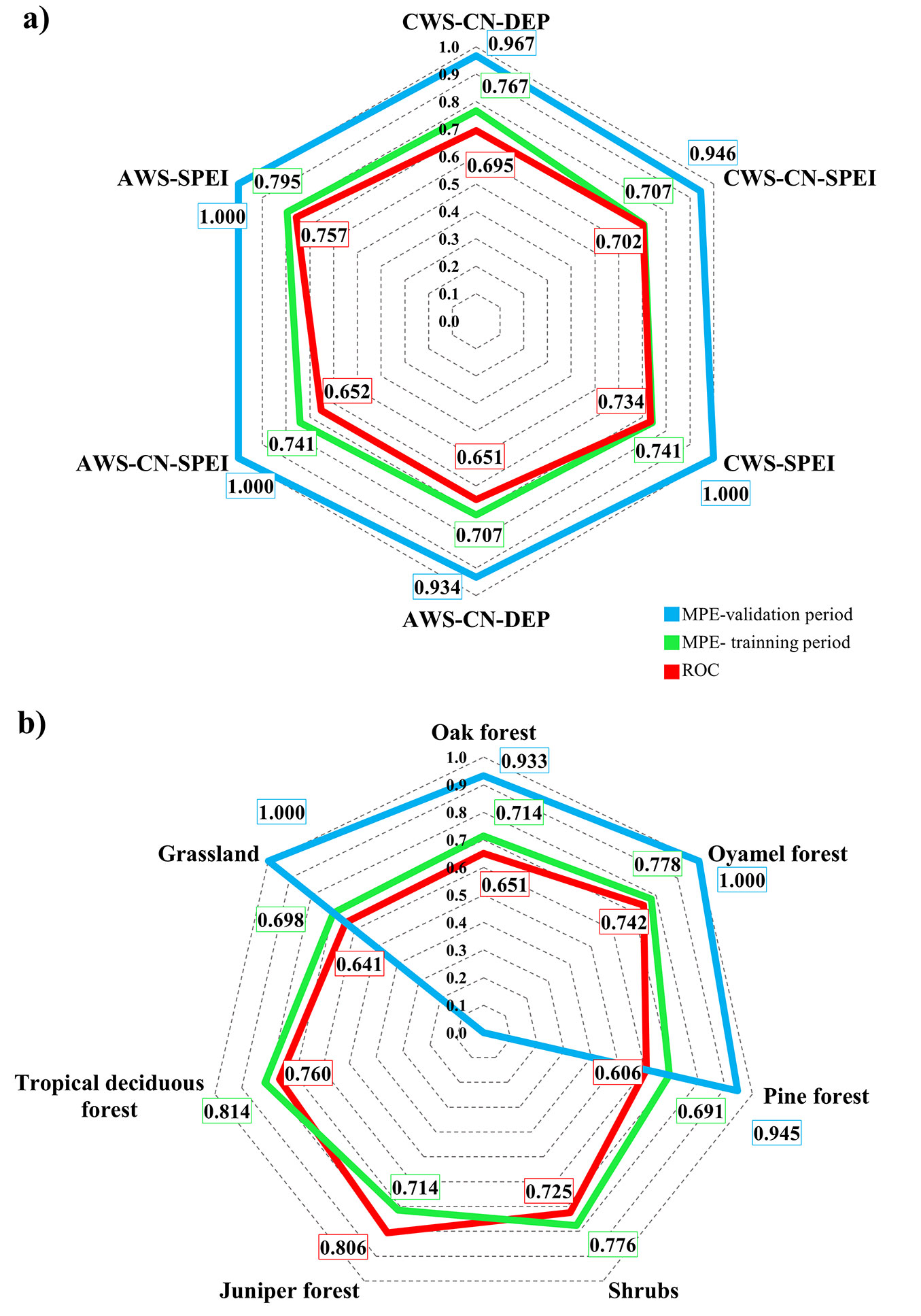
Overall, 252 LRMs were built to predict daily fire ignition, resulting from the combination of drought indices (EDI and SPEI) and weather data sources (CWS and AWS) applied monthly for each of the 7 types of vegetation cover. Tab. S1 (Supplementary material) reports the median monthly ROC and MPE values of each model, grouped in 6 LRM classes (CWS-CN-DEP, CWS-CN-SPEI, CWS-SPEI, AWS-CN-DEP, AWS-CN-SPEI, and AWS-SPEI) and seven types of vegetation cover (oak forest, oyamel forest, pine forest, shrubs, juniper forest, tropical deciduous forest, and grassland). The median values reported in Tab. S1 were used to build the diagrams in Fig. 4.
Fig. 4 - ROC and MPE results of the 252 logistic regression models (LRMs) developed for daily prediction of forest fire ignition based on meteorological drought indices. (a) LRMs were grouped in 6 classes (CWS-CN-DEP, CWS-CN-SPEI, CWS-SPEI, AWS-CN-DEP, AWS-CN-SPEI, and AWS-SPEI), with median ROC values represented in red, MEP for the training period in green, and MPE for the validation period in blue. (b) LRMs were grouped by type of vegetation cover (oak forest, oyamel forest, pine forest, shrubs, juniper forest, tropical deciduous forest, and grassland), with median ROC values represented in red, MEP for the training period in green, and MPE for the validation period in blue. The median values displayed are also reported in Tab. S1 (Supplementary material).
AWS-SPEI models showed the best performances (Fig. 4a), with median ROC = 0.757 (red diagram in Fig. 4a). Close performances were showed by CWS-SPEI models, with a median ROC value of 0.734. The full list of median ROC values for the 252 monthly models is reported in Tab. S1 (Supplementary material). The best results for each month of the fire season were obtained using the following models: January CWS-SEPI (0.742), February AWS-SPEI (0.821), March AWS-SPEI (0.751), April CWS-CN-SPEI (0.748), May CWS-CN-SPEI (0.778), and June CWS-SPEI (0.742). Any combination of LRM with SPEI had outstanding ROC values, as depicted in Fig. 4a.
For the training period, the maximum MPE value (0.795) was obtained using the AWS-SPEI model (green diagram in Fig. 4a). Monthly MPE results (Tab. S1 in Supplementary material) showed that the best models for January were CWS-CN-DEP (median MPE = 0.767), for April the CWS-CN-DEP and CWS-SPEI models (median MPE = 0.769), while for February, March, May, and June, the best performances were shown by the AWS-SPEI models (median MPE = 0.833, 0.778, 0.802 and 0.810, respectively). In general, all LRMs evaluated over the training period had MPE > 0.700.
One of the main problems presented by LRMs was the small amount of matching fire and weather data for the validation period (2015). Indeed, the number of fire occurrence in at least one type of vegetation in the validation dataset was only 307. Despite the little dataset, the validation results were outstanding for all LRMs, with values greater than 0.940 (blue diagram in Fig. 4a). Monthly validation shows that the six types of LRMs had median MPE values greater than 0.880 for February and April, except for AWS-CN-DEP which had median MPE = 0.723 in February (see also Tab. S1 in Supplementary material). As for January, only CWS-CN-SPEI models had sufficient data for validation. The month of May had MPE values < 0.800, still indicating a satisfactory accuracy in the prediction of fire occurrence. The month of June did not provide sufficient data for the validation of LRMs, although an increase in humidity is observed in June due to the beginning of the rainy period in the Mexican highlands. However, all LRMs showed outstanding performances (MPE > 0.700) over the validation period.
Effects by weather data source and vegetation cover
ROC results for LR modeling periods (Fig. 4a) generally show that CWS models had better performances in predicting fire occurrence with maximum certainty values (two CWS and one AWS models with ROC ≥ 0.700). Moreover, Tab. S1 shows that CWS monthly models had better performances (9 models with ROC ≥ 0.700) as compared with AWS models (7 models exceeding the 0.700 threshold). Also, 5 AWS models had minimum ROC values in their monthly pool (ROC< 0.600).
Fig. 4b and Tab. S1 show the ROC results of the 252 LRMs summarized by vegetation cover (red diagram in Fig. 4b). The best performing LRMs were those for the juniper forest (median ROC = 0.806), tropical deciduous forest (ROC = 0.760), oyamel forest (ROC = 0.742), and shrubland (ROC = 0.725). Meanwhile, the predictions were less accurate for oak forest (median ROC = 0.651), grassland (ROC = 0.641), and pine forest (ROC = 0.606). The diagram in green color of Fig. 4b presents the MPE results of the 252 LRMs in the training period grouped by type of vegetation. The outstanding models with MPE ≥ 0.700 were tropical deciduous forest (MPE = 0.814), oyamel forest (MPE = 0.778), shrubs (MPE = 0.776), oak forest and juniper forest (both MPE = 0.714). Although grassland (MPE = 0.698) and pine forest (MPE = 0.691) vegetation types had MPE < 0.700, it is judged that all coverages showed outstanding results at the training stage. Finally, the diagram in blue color in Fig. 4b shows that the LRMs had outstanding efficiency in the validation period (MPE ≥ 0.900) for all types of vegetation (Tab. S2 and Tab. S3 in Supplementary material). Specifically, Tab. S2 provides monthly ROC and MPE values and Tab. S3 shows the coefficients for daily fire prediction in Mexican highlands.
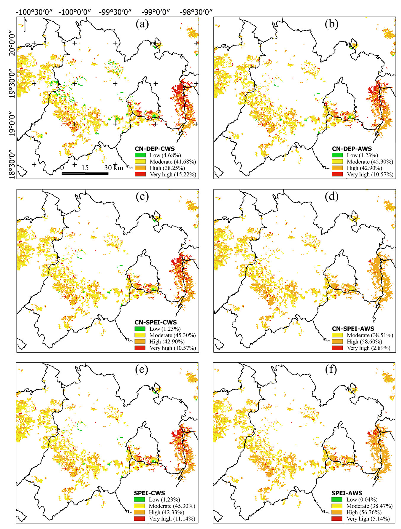
An example of the application of the six LRMs (CWS-CN-DEP, CWS-CN-SPEI, CWS-SPEI, AWS-CN-DEP, AWS-CN-SPEI, and AWS-SPEI) in the Mexican highlands is reported in Fig. 5(a-f) where the ignition hazard for April 5th, 2012 is shown. In general, all LRMs predicted a high ignition danger (categories “very high” and “high”) in the western part of the study area (Fig. 5a to Fig. 5f). According to PROBOSQUE, these sites are most frequently affected by wildfires every year. These areas correspond to the highest altitude lands, near the two highest volcanoes of Mexico. The dominant vegetation of these areas are pine, oyamel, and oak forests, which due to their proximity to urban areas, are of interest for the environmental services they provide.
Fig. 5 - Example of the application of the six logistic regression models (LRMs) developed for the Mexican highlands on April 5th, 2012. The probability of fire occurrence (P), grouped in 4 fire hazard classes, is shown: low (green pixels), moderate (yellow pixels), high (orange pixels), and very high (red pixels). The percentage of the potentially ignitable area for each fire hazard class is given in brackets.
Discussion
LRMs and explanatory variables for daily fire prediction
The construction of 252 LRMs for fire prediction has taken into account the geographical, biophysical and climatic aspects of the studied region, with the aim of obtaining specific models for each month in the fire season and each type of vegetation in the Mexican highlands. Such objective is consistent with current approach of developing fire prediction tools in homogeneous areas with low temporality ([24]). In addition, modeling was applied on a regional scale in Mexico, and allow to analyze the impacts of fires on local natural resources ([11]). Furthermore, the LRMs presented in this study had high spatial resolution (pixel area of 1 km2). It has been demonstrated that the longer lead time prediction and the higher the spatial resolution, the lower is the level of accuracy attained in fire prediction ([23]). However, it should be noted that previous studies used spatial scales between 10 and 20 km ([38], [28], [23]), and the choice of these scales makes it challenging to take decisions at the operational level.
Fuel dryness variables in the proposed LRMs had a small (daily) time scale, which is recommended when weather data are integrated into fire prediction models ([5]), as annual climate estimates have been shown to have a negligible contribution in forecasting models ([19]).
The level of accuracy of fire prediction models lies in selecting independent variables that efficiently explain the occurrence of fires. In this study we included in LRMs several independent variables which have been previously reported as the most influential in fire ignition and propagation ([43]). Indeed, these variables have often been used as excellent fire predictors in previous work: (i) fuel dryness, as indicated by Martell et al. ([24]), Vega et al. ([38]), and Ali et al. ([2]); (ii) climatic aspects, as employed by Vega et al. ([38]), Padilla & Vega-García ([28]), Magnussen & Taylor ([23]), Guo et al. ([16]), and Rodrigues et al. ([32]); (iii) geographical aspects, as indicated in the results of Vega et al. ([38]), Padilla & Vega-García ([28]), and Hong et al. ([19]); and (iv) human-related aspects (e.g., infrastructures), as analyzed by Vega et al. ([38]), Magnussen & Taylor ([23]), Arndt et al. ([5]), Guo et al. ([16]), and Rodrigues et al. ([32]). Nonetheless, some LMR in this study had prediction efficiency lower (or little exceeding) than the set threshold (ROC ≥ 0.700), likely due to some level of collinearity between the explanatory variables.
In general, most of the proposed LRMs showed a sufficient level of efficiency (median ROC ≥ 0.734 and median MPE ≥ 0.943) to recommend their use in the prediction of fire occurrence, as reported by Martínez et al. ([25]), Madrigal et al. ([22]), Vilar et al. ([42]), Pacheco et al. ([27]), Carrillo et al. ([8]), Guns & Vanacker ([14]), Guo et al. ([16]), Rodrigues et al. ([32]), and Turco et al. ([36]). Also, in this study we have chosen LRMs as easy and suitable tools for forest fire management, according to Andrews et al. ([4]) and Guo et al. ([15]).
Drought indices as fuel dryness estimators
We built 252 LRMs with their respective fuel dryness thresholds to model fire occurrence in an area characterized by a significant climatic and topographic heterogeneity (Fig. 1). This is consistent with the conclusions of Aguado & Camia ([1]), who stated that it is difficult to establish a single drought threshold for heterogeneous areas in terms of climate and geography. Although in this study SPEI was calculated on a daily basis with satisfactory results, Turco et al. ([36]) estimated SPEI over 3, 6, and 12 months, obtaining the best fire predictions for SPEI calculated over more than two months. Vélez ([39]) and McEvoy et al. ([26]) mentioned that using evapotranspiration in drought indices the moisture status in light fuels (branches and leaves) is better estimated. This was considered in this study by including SPEI in predicting the dryness of potentially flammable fuels (Fig. 4a, Fig. 4b). As previously reported, the relationship between SPEI and forest fires is very high ([37], [17], [26]).
Limitations
The LRMs with the lower predictive efficiency were obtained for those types of vegetation which are most represented in the study area (pine forest: ROC = 0.606, MPE = 0.691; grassland: ROC = 0.641, MPE = 0.698; oak forest: ROC = 0.651 - Fig. 1, Fig. 4b). It is recommended to further enhance the LRMs for these areas, since some collinearity may exist in the analyzed dataset between anthropogenic, meteorological, and geographical explanatory variables ([14], [32], [36]), despite the conclusions of Vilchis-Francés et al. ([43]). Indeed, it is important to reduce or remove the possible collinearity between biophysical and social factors involved in fire initiation and propagation. Therefore, future studies should be aimed to select as predictors in LRMs the first orthogonal components of PCA related to the previously selected explanatory variables ([28], [15], [16]).
This study used the SPEI drought index on a daily basis, which was appropriate for estimating the moisture content in light fuels, as indicated by Vélez ([39]). However, it is also necessary to consider the moisture content in heavier fuels if SPEI is calculated with weather data aggregated over 15 days or more, such as the previous drought accumulation (CN-DEP and CN-SPEI models). Similarly, a slight correlation was detected between the weather data sources (CWS and AWS) used to generate the estimates of potentially combustible fuel dryness; however, when results are considered on a monthly basis, CWS models were more efficient in predicting fires. This better efficiency could be due to the high sensitivity of the prediction models to weather data variability. Indeed, a variation in the spatial and temporal distribution of precipitation and temperature can lead to significant differences among model predictions. It is assumed that the lower the daily variability in weather data, the higher the ROC values of the LRM. Due to the limited data availability for validation, it was not possible to conduct certainty assessments for LRMs in hedges that had high fire prediction efficiencies, such as shrubland (ROC = 0.725, MPE = 0.776), juniper forest (ROC = 0.806, MPE = 0.714), and tropical deciduous forest (ROC = 0.760, MPE = 0.814). It would certainly be advisable for government institutions to further increase the information collected to improve the construction of predictive models and strengthen the proportion of data for modeling (70% to 80%) and validation (20% to 30%).
Conclusions
In this study 252 monthly LRMs for daily fire ignition prediction were developed using different sources of weather data (AWS and CWS) and drought indices (EDI and SPEI) to estimate fuel dryness (CN-DEP, CN-SPEI, and SPEI) in selected types of vegetation in the Mexican highlands. The exhaustive dataset led to the creation of six types of LRM (CWS-CN-DEP, CWS-CN-SPEI, CWS-SPEI, AWS-CN-DEP, AWS-CN-SPEI, and AWS-SPEI). Based on our results, we suggest the use of high-density CWS weather data sources, as they offer greater certainty in generating predictors of potentially ignitable fuel dryness. On the other hand, a disadvantage of CWS networks is that they do not generate data as rapidly as AWS networks. For both weather data sources, the SPEI drought index is recommended to estimate fuel dryness, as SPEI reflects the balance between precipitation and reference evapotranspiration, while EDI is based on the former variable only. Moreover, our results showed that SPEI is better than CN-SPEI at estimating fuel dryness, though they come from the same SPEI index. Finally, counting the days of moisture deficit does not fully represent the magnitude of this deficit.
Further studies aimed to improve daily fire prediction models should be focused on the use of satellite images of soil and vegetation moisture as dynamic predictors. Moreover, the optimization of the spatial scale of models is desirable in order to improve the prediction accuracy. Finally, we advise a faster release of CWS data (currently available after six months) and highlight the need of extending AWS spatial coverage in the study area.
List of Abbreviations
(AWS): Automatic Weather Station; (AWS-CN-DEP): CN-DEP model with AWS data source; (AWS-CN-SPEI): CN-SPEI model with AWS data source; (AWS-SPEI): SPEI model with AWS data source; (CN-DEP): Consecutive days of Negative deviation from effective precipitation DEP; (CN-SPEI): Consecutive days of Negative SPEI index; (CONAFOR): National Forestry Commission in Mexico; (CWS): Conventional Weather Station; (CWS-CN-DEP): CN-DEP model with CWS data source: (CWS-CN-SPEI): CN-SPEI model with CWS data source; (CWS-SPEI): SPEI model with CWS data source; (DEM): Digital Elevation Model; (DEP): Deviation from Effective Precipitation EP; (EDI): Effective Drought Index; (EP): Effective Precipitation; (ETP): Reference Evapotranspiration; (LRM): Logistic Regression Model; (MODIS): Moderate Resolution Imaging Spectroradiometer; (MPE): Model Precision Efficiency; (NASA): National Aeronautics and Space Administration; (P): Probability of occurrence; (p): Precipitation; (PCA): Principal Component Analysis; (PROBOSQUE): Forest Protector of the State of Mexico; (ROC): Relative Operating Characteristic; (SPEI): Standardized Precipitation-Evapotranspiration Index.
Acknowledgments
Thanks to the Fiducie de Recherche en Hydrologie (Quebec-Canada) - UAEMex 4212/ 2016E, the Consejo Nacional de Ciencia y Tecnología - CONACyT 248498, the Instituto Interamericano de Tecnología y Ciencias del Agua de la Universidad Autónoma del Estado de México, the Red Lerma group, as well as the Protectora de Bosques del Estado de México for the respective supports to this work.
Funding
This study was supported by the following projects: (i) Análisis de sequía y diseño de una herramienta hidrogeomática como soporte para la toma de decisiones (UAEMex 4212/2016E) sponsored by the Fiducie de Recherche en Hydrologie, Quebec, Canada; (ii) Modelo de base hidroclimatológica para la identificación en tiempo real de áreas susceptibles a peligro de ignición como apoyo a la protección de ecosistemas y su biodiversidad (CONACyT 248498) sponsored by the Consejo Nacional de Ciencia y Tecnología of Mexico.
References
Gscholar
Online | Gscholar
CrossRef | Gscholar
Gscholar
Online | Gscholar
Online | Gscholar
Gscholar
Gscholar
Online | Gscholar
Authors’ Info
Authors’ Affiliation
Carlos Díaz-Delgado
Rocío Becerril Piña
Carlos Alberto Mastachi Loza 0000-0001-9516-1170
Miguel Ángel Gómez-Albores 0000-0002-6313-9187
Khalidou M Bâ 0000-0003-1710-5653
Instituto Interamericano de Tecnología y Ciencias del Agua, Universidad Autónoma del Estado de México - IITCA/UAEMex (México)
Carlos Díaz-Delgado
Rocío Becerril Piña
Red Interinstitucional e Interdisciplinaria de Investigación, Consulta y Coordinación Científica para la Recuperación de la Cuenca, Lerma-Chapala-Santiago-IITCA-UAEMex, Red Lerma (México)
Corresponding author
Paper Info
Citation
Vilchis-Francés AY, Díaz-Delgado C, Becerril Piña R, Mastachi Loza CA, Gómez-Albores MÁ, Bâ KM (2021). Daily prediction modeling of forest fire ignition using meteorological drought indices in the Mexican highlands. iForest 14: 437-446. - doi: 10.3832/ifor3623-014
Academic Editor
Davide Ascoli
Paper history
Received: Aug 11, 2020
Accepted: Jul 28, 2021
First online: Sep 28, 2021
Publication Date: Oct 31, 2021
Publication Time: 2.07 months
Copyright Information
© SISEF - The Italian Society of Silviculture and Forest Ecology 2021
Open Access
This article is distributed under the terms of the Creative Commons Attribution-Non Commercial 4.0 International (https://creativecommons.org/licenses/by-nc/4.0/), which permits unrestricted use, distribution, and reproduction in any medium, provided you give appropriate credit to the original author(s) and the source, provide a link to the Creative Commons license, and indicate if changes were made.
Web Metrics
Breakdown by View Type
Article Usage
Total Article Views: 34470
(from publication date up to now)
Breakdown by View Type
HTML Page Views: 28599
Abstract Page Views: 2409
PDF Downloads: 2849
Citation/Reference Downloads: 6
XML Downloads: 607
Web Metrics
Days since publication: 1689
Overall contacts: 34470
Avg. contacts per week: 142.86
Article Citations
Article citations are based on data periodically collected from the Clarivate Web of Science web site
(last update: Mar 2025)
(No citations were found up to date. Please come back later)
Publication Metrics
by Dimensions ©
Articles citing this article
List of the papers citing this article based on CrossRef Cited-by.
Related Contents
iForest Similar Articles
Research Articles
Comparison of drought stress indices in beech forests: a modelling study
vol. 9, pp. 635-642 (online: 06 May 2016)
Research Articles
Impact of climate change on tree-ring growth of Scots pine, common beech and pedunculate oak in northeastern Germany
vol. 9, pp. 1-11 (online: 13 October 2015)
Research Articles
Probabilistic prediction of daily fire occurrence in the Mediterranean with readily available spatio-temporal data
vol. 10, pp. 32-40 (online: 06 October 2016)
Research Articles
The response of intra-annual stem circumference increase of young European beech provenances to 2012-2014 weather variability
vol. 9, pp. 960-969 (online: 23 June 2016)
Research Articles
Evaluation and correction of optically derived leaf area index in different temperate forests
vol. 9, pp. 55-62 (online: 11 June 2015)
Research Articles
Remote sensing of Japanese beech forest decline using an improved Temperature Vegetation Dryness Index (iTVDI)
vol. 4, pp. 195-199 (online: 03 November 2011)
Research Articles
Do different indices of forest structural heterogeneity yield consistent results?
vol. 15, pp. 424-432 (online: 20 October 2022)
Research Articles
Estimation of forest leaf area index using satellite multispectral and synthetic aperture radar data in Iran
vol. 14, pp. 278-284 (online: 29 May 2021)
Research Articles
Assessment of age bias in site index equations
vol. 9, pp. 402-408 (online: 11 January 2016)
Research Articles
Drought effects on the floristic differentiation of Greek fir forests in the mountains of central Greece
vol. 8, pp. 786-797 (online: 08 April 2015)
iForest Database Search
Google Scholar Search
Citing Articles
Search By Author
Search By Keywords

