Estimation of forest leaf area index using satellite multispectral and synthetic aperture radar data in Iran
iForest - Biogeosciences and Forestry, Volume 14, Issue 3, Pages 278-284 (2021)
doi: https://doi.org/10.3832/ifor3633-014
Published: May 29, 2021 - Copyright © 2021 SISEF
Research Articles
Abstract
Different satellite datasets, including multispectral Sentinel 2 and synthetic aperture radar Sentinel 1 and ALOS2, were tested to estimate the Leaf Area Index (LAI) in the Zagros forests, Ilam province, in Iran. Field data were collected in 61 sample plots by hemispherical photographs, to train and validate the LAI estimation models. Different satellite data combinations were used as input in regression models built with the following algorithms: Multiple Linear Regression, Random Forests, and Partial Least Square Regression. The results indicate that Leaf Area Index can be best estimated using integrated ALOS2 and Sentinel 2 data; these inputs generated the model with higher accuracy (R2 = 0.84). The combination of a single band and a vegetation index from Sentinel 2 also led to successful results (R2 = 0.81). Lower accuracy was obtained when using only ALOS 2 (R2 = 0.72), but this dataset is helpful where cloud coverage affects optical data. Sentinel 1 data was not useful for LAI prediction. The optimal model was based on the traditional Multiple Linear Regression algorithm, using a preliminary input selection step to exclude multicollinearity effects. To avoid this step, the use of Partial Least Square Regression may be an alternative, as this algorithm was able to produce estimates similar to those obtained with the best model.
Keywords
Introduction
The extraction of spatially and temporally explicit vegetation bio-geophysical variables is required in a variety of ecological and agricultural applications ([48]). Leaf Area Index (LAI) is defined as half the total intercepting leaf area per unit of ground surface, projected on the local horizontal datum ([6]). LAI is a dimensionless value typically ranging from 0, for bare ground, to more than 7 for dense vegetation, and is an important structural parameter related to many forest stand processes, such as photosynthesis, respiration, rainfall interception, carbon and nutrient cycles ([47]). LAI is also related to stands health, being linked to leaf and canopy chlorophyll contents, dry and fresh biomass, and growth stages ([50]). LAI is frequently used by foresters and ecologists to simulate ecological processes, as well as by agronomists and crop modelers to model crops dynamics and productivity, and is one of the most important indices to monitor vegetation status and estimate productivity ([29]). Although direct measurements of canopy LAI give relatively precise values, data collection is time-consuming and labor-intensive, and only feasible in small-scale plots. Remote sensing-based LAI estimates now complement the ground measurements, thanks to the capability of remote data to cover large extents repeatedly in time, and generate LAI estimated values at local and global scales.
Several approaches are available to estimate LAI using remote sensing methods. The gap fraction method ([34]) is based on the use of below canopy hemispherical images and is often adopted at local or stand scale to collect LAI information, due to its fast and non-destructive nature. The hemispherical photographs capture the patterns of light obstruction/penetration in the canopy, from which the canopy architecture and foliage area can be quantified ([16]); LAI and other canopy properties are estimated through the measurement of radiation transmitted through the canopy and the application of radiative transfer models ([38]). In recent years, digital hemispherical photography has received increasing attention as an inexpensive tool for near-surface remote sensing of forest canopy structure, with research carried out in multiple environments ([4], [52], [14]).
Other studies were based on the use of satellite multispectral data for LAI prediction, exploiting the direct relationship that links canopy reflectance values with foliage density ([27], [48]). However, the availability of optical data is often hampered by the presence of cloud coverage. Indeed, a saturation of reflectance response is observable at high LAI values, and consequently no information can be gathered about the understory vegetation or the woody stand structure ([44]).
To cope with the limitations occurring in optical data, microwave Synthetic Aperture Radar (SAR) data were adopted in agricultural and forestry research for LAI estimation. SAR data are insensitive to cloud and day/night conditions. Furthermore, the intensity of the backscattered SAR signal is related to the target volume and its water content, with the penetration of SAR depending on the wavelength used. Usually, at L- and P-long wavelengths the signal penetration into the vertical profile is high, and SAR can sense the different vegetation strata. At shorter wavelength, such as C-band, the information mainly comes from the upper canopy layer ([41]).
Multiple examples are reported in the literature about the use of SAR data, mainly C-band, to estimate LAI in different crops ([25], [24], [31]), as well as in grasslands ([30]). Yet, fewer studies were carried out in forest environments. In the Amazon varzea forest, Pereira et al. ([35]) used different SAR sensors including ALOS PALSAR at L-band to retrieve both above ground biomass and LAI, showing that ALOS PALSAR provided the best estimates of both variables with respect to other SAR datasets. Stankevich et al. ([42]) developed a method for LAI estimation in temperate deciduous and mixed forests using Sentinel 1 at C-band. Chen et al. ([7]) compared the performances of various optical sensors with those of ALOS PALSAR for LAI estimation, showing that the addition of SAR brought new information in the optical-based LAI regression model, and suggested the combined use of optical AVNIR-2 and microwave PALSAR, that are on the same ALOS platform. Manninen et al. ([32]) developed a method for assessing LAI in boreal forests using ENVISAT C-band SAR data polarization ratio (VV/HH); using the same sensor, Gao et al. ([17]) evidenced the sensitivity of SAR backscattering at different polarizations to LAI in poplar and desert date forest plantations in China.
The objective of this study was to compare the single and combined use of multispectral and SAR data for LAI estimation in a Mediterranean forest site. Specifically, the use of SAR was tested to offer an alternative to multispectral data when cloud coverage affects the quality of optical imagery. Different algorithms were tested, including Multilinear Regression, Random Forests, and Partial Least Squared Regression, to improve the accuracy of results and to facilitate the processing task. The results were rigorously validated and compared to each other to offer a perspective on LAI estimation in forest analysis.
Methods
Study area
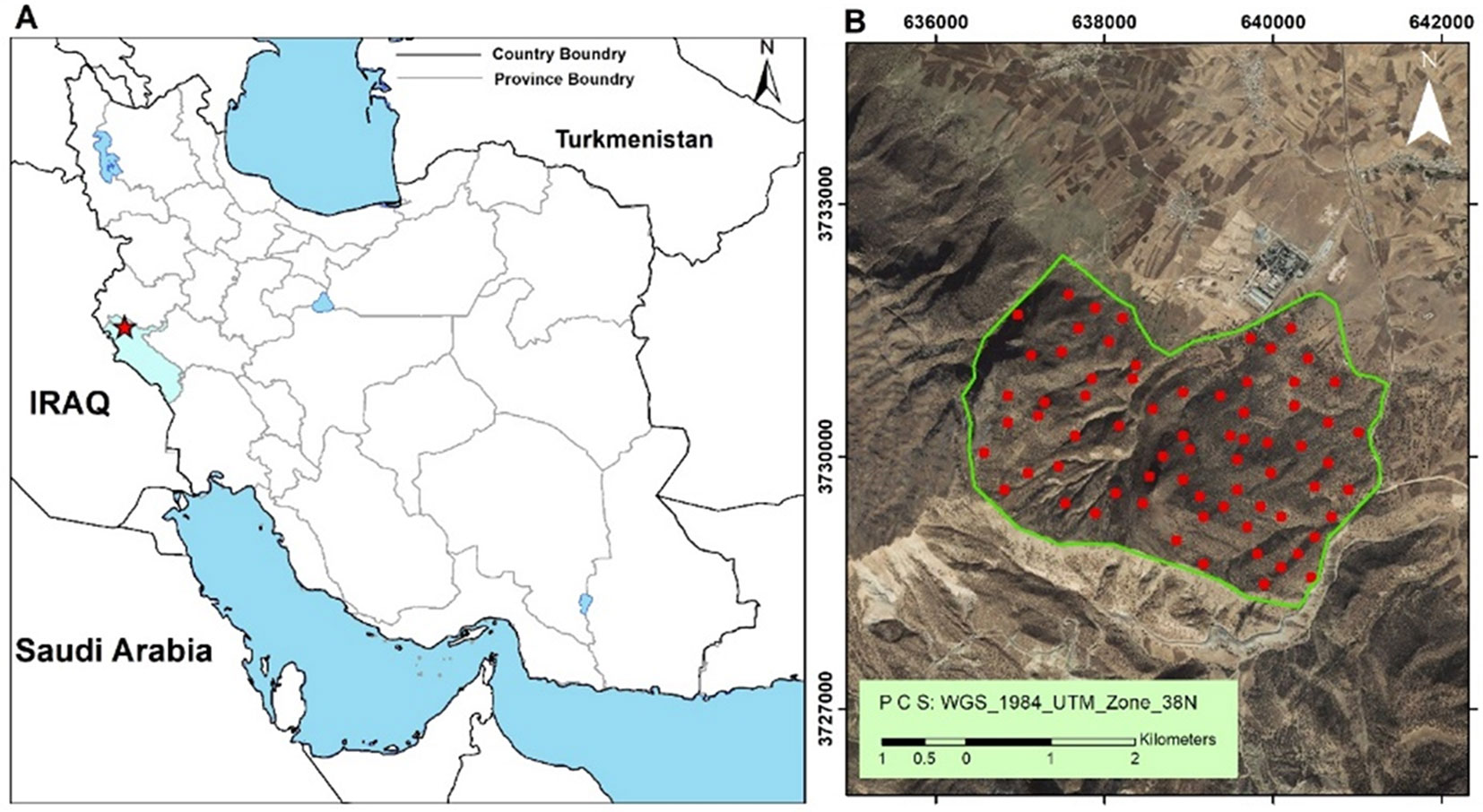
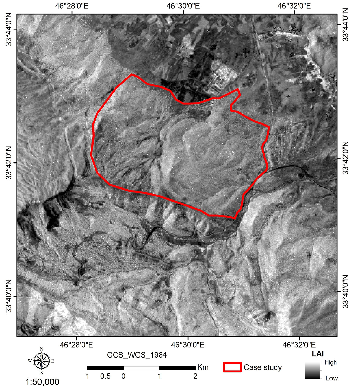
The study was carried out in the Southern Zagros protected forest, in the Dalab region of the western Iranian state of Ilam (Fig. 1). This is a sub-Mediterranean region, characterized by marked seasonality in rainfall distribution. The altitude ranges from approximately 1300 to 2200 m a.s.l., with average slopes equal to 17°. The main woody species in this area is the Brant’s oak (Quercus brantii), usually found in pure stands and covering about 3.5 million hectares in Zagros. Other species that are often present include: Pistacia atlantica, Acer spp., Crataegus azarolus, Cerasus microcarpa, Daphne mucronate, Amygdalus orientalis, Lonicera nummularifolia. The density of stands varies across the study area, in the range of 30-100 trees per hectare; the average forest coverage is about 45%. Seasonally, the ground is covered by grasses ([40]).
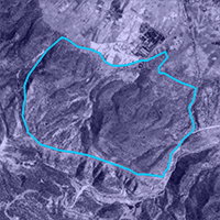
Fig. 1 - (A) Geographic location of the study area (red star); (B) location of the field plots (red dots).
Satellite data
Three different satellite datasets were used: (i) multispectral Sentinel 2 (L1C1) dated July 23, 2016; (ii) SAR Sentinel 1 (L1C HRD) dated June 8, 2016; and (iii) ALOS2 (level 1.1 SLC), dated June 23, 2016. Satellite data processing was carried out in SNAP, the free processing facilities offered by the European Space Agency (ESA - ⇒ http://step.esa.int/main/toolboxes/snap/).
The Sentinel 2 (S2) instrument samples 13 spectral bands in the visible-near infrared (VIS-NIR) to the shortwave infrared (SWIR) range, with four bands at 10 m, six bands at 20 m and three bands at 60 m spatial resolution; it also incorporates three bands in the red-edge region, centered at 705, 740 and 783 nm. The S2 image was atmospherically corrected using the ESA Sen2Cor algorithm. For the present study, ten original bands at 10-20 m spatial resolution and 22 vegetation indices listed in Tab. S1 (Supplementary material) were used as inputs in models to predict LAI.
Sentinel 1 (S1) is an SAR constellation equipped with C-band sensors and has a 6 day repeat cycle. For this research, the Sentinel-1A Interferometric Wide swath mode (IW), Level-1 Ground Range Detected (GRD) scene with dual-polarization (VV and VH) was used. The scene has a pixel spacing equal to 10 m and an incidence angle of approximately 39-40°; it was calibrated, filtered with the refined Lee filter to reduce speckle noise, and terrain corrected using the SRTM-1 sec DEM (Shuttle Radar Topography Mission-3 Digital Elevation Model), to produce a regular grid of 20 m spatial resolution size. Finally, it was co-registered with the Sentinel-2 scene. The two VV and VH polarizations were used as input in models to predict LAI.
The Advanced Land Observing Satellite-2 (ALOS-2) carries on the PALSAR2 L-band SAR sensor. Level 1.1 data single look complex (SLC) fine beam scene, in HH and HV polarizations with an incidence angle of 34.3°, and 12.5 m pixel spacing were acquired, multilooked, filtered for speckle noise using the refined Lee filter, and terrain corrected using the SRTM-1 sec DEM. The final spatial resolution was set to 20 m and the scene was co-registered with the Sentinel-2 image.
Field plots
Sixty-one plots of 40 × 40 m were set up in the study area, recording their center with a GPS device eTrex® 20 (Garmin, Schaffhausen, Switzerland). In each plot, a 4 × 3 grid defined 12 points, each being 8-10 m apart from the neighboring one: the points corresponded to locations where digital hemispherical photographs (DHP) images were collected at sunrise under uniform sky conditions. The DHP were collected using a digital camera (EOS® 6D, Canon, Tokyo, Japan) fitted with a fisheye adapter lens (EF Lens 24-105mmF4 L IS USM, Canon, Tokyo, Japan). LAI was calculated from the DHP images using the Gap Light Analyzer software, based on the Beer-Lambert Law and the Miller equation for foliage density ([33]).
Data analysis and modeling
The pixels included in the field plot areas were extracted from the different optical (S2) and microwave (S1 and ALOS2) satellite datasets. Pixels were averaged at plot level, obtaining the reflectance and the backscattering values of each plot. A preliminary correlation analysis showed high correlation of field LAI values with different satellite data.
The most relevant predictors (p<0.05) from S1, S2, and ALOS2 datasets were identified through stepwise regression (alpha to enter and remove = 0.15 - Tab. 1). The stepwise procedure allows the number of inputs in models to be reduced, thereby avoiding multicollinearity effects, or inflating the regression models.
Tab. 1 - Input’s data in stepwise regression. (§): see Tab. S1 in Supplementary material.
| Dataset | Variables | Number of inputs |
|---|---|---|
| Sentinel 2 | Bands: B2, B3, B4, B5, B6, B7, B8, B8a, B11, and B12; 17 Vegetation Indices § |
32 |
| Sentinel 1 | VH, VV, VV/VH, VH+VV, VH-VV | 5 |
| ALOS 2 | HH, HV, HH/HV, HH+HV, HH-HV | 5 |
Three different algorithms were used to build the LAI regression models. The first, Multiple Linear Regression (MLR), is a statistical technique that exploits several explanatory variables to predict the outcome of a response variable, widely used in forest research for its simplicity of application; basically, it is an extension of the ordinary least-squares (OLS) regression that involves more than one explanatory variable ([15]).
The second algorithm, Random Forests (RF), is a supervised “ensemble learning” method able to cope with complex datasets ([3]). RF generates many regression trees (models) and aggregates their results, exploiting the bootstrap aggregation method, reducing the output variance and of the overfitting problem. The n-trees and the m-try are the only two parameters that must be chosen to train the RF model, making its application smoother when compared to more complex machine learning algorithms. During the training phase, each tree is built by a growing process implementing different cascaded nodes, representing the ramification of a tree. Data kept separate from the training subsets are called “Out-Of-Bag” (OOB) samples and are used to validate the model and define the associated OOB error, also called the “Out-Of-Bag estimate”. The latter is the mean prediction error on each training sample, computed using only the trees that did not include the same samples in their bootstrap dataset ([3]). Random Forests is commonly applied in remote sensing and forest ecology ([49]).
Finally, Partial Least Squared Regression (PLSR), closely related to principal component regression, was selected as an additional algorithm given its ability to deal with multicollinearity issues and the “curse of dimensionality”. PLSR uses the information from the response variable in addition to the predictors for feature transformation ([18]); this algorithm is commonly used in ecological and forestry applications exploiting large, complex datasets ([46]).
LAI estimation models were first built using the inputs selected by stepwise regression, setting three Multiple Linear Regression models: MLR M1 using multispectral data, MLR M2 using SAR data, and MLR M3 using integrated optical-SAR datasets. MLR M3 input data - characterized by different optical and SAR physical properties - were then used as input in the Random Forests algorithm (named RF M4). Finally, to avoid running a preliminary stepwise regression, all the available predictors were used as input in Partial Least Squared Regression algorithm (models named PLSR M5, PLSR M6, PLSR M7). PLSR was also run using the stepwise selected optical and SAR inputs (model PLSR M8), for comparison purposes with MLR M3 and RF M4. All the models were validated with 10-fold cross validation (Tab. 2). MLR and RF models were evaluated by the coefficient of determination (R2) and the Root Mean Squared Error (RMSE) statistical metrics; PLSR models were evaluated using the R2 and the PRESS statistics (minimum predicted residual sum of squares).
Tab. 2 - Algorithms and input data used in the different regression tests.
| Model | Algorithm | Variables | Number of inputs |
|---|---|---|---|
| MLR M1 - multispectral | Multiple Linear Regression | B4, ARVI | 2 |
| MLR M2 - SAR | Multiple Linear Regression | ALOS2 HV | 1 |
| MLR M3 - multispectral + SAR | Multiple Linear Regression | B4 + ARVI + ALOS2 HV | 3 |
| RF M4 - multispectral + SAR | Random Forests | B4 + ARVI + ALOS2 HV | 3 |
| PLSR M5 - multispectral | Partial Least Squared Regression | 10 S2 bands + 22 vegetation indices (as in Tab. 1) | 32 |
| PLSR M6 - SAR | Partial Least Squared Regression | 5 S1 + 5 ALOS2 inputs (as in Tab. 1) | 10 |
| PLSR M7 - multispectral + SAR | Partial Least Squared Regression | 10 S2 bands + 22 vegetation indices + 5 ALOS 2 inputs (as in Tab. 1) | 37 |
| PLSR M8 - selected multispectral + SAR | Partial Least Squared Regression | B4 + ARVI + ALOS2 HV | 3 |
Using the most accurate model, a map of estimated LAI was generated for the entire study area.
Results
The summary statistics of the LAI measured in sample plots shows that LAI values for the site are normally distributed, and range between 0.59-2.66 (Tab. 3). The results of Pearson’s correlation analysis between LAI and the various satellite predictors are presented in Tab. 4; the relationships were consistently linear.
Tab. 3 - Descriptive statistics of LAI measured in the study plots (N = 61).
| Statistics | Value |
|---|---|
| Minimum | 0.59 |
| Maximum | 2.66 |
| Mean | 1.66 |
| Std. Deviation | 0.52 |
Tab. 4 - Pearson’s correlation coefficients between LAI and satellite predictors. (*): p<0.05; (**): p<0.01.
| Dataset | Bands /indices | r | Bands / indices | r | Bands / indices | r |
|---|---|---|---|---|---|---|
| Sentinel 2 | B2 | -0.765* | PVI | 0.767* | WDVI | 0.750* |
| B3 | -0.790* | RVI | 0.590* | Tsavi | 0.834* | |
| B4 | -0.888* | NDVI | 0.882* | ARVI | 0.828* | |
| B5 | -0.797** | DVI | 0.767* | NDI45 | -0.404** | |
| B6 | -0.682** | GNDVI | 0.759* | REIP | -0.169 | |
| B7 | -0.603** | IPVI | 0.882* | IRECI | 0.799** | |
| B8a | -0.561* | Msavi | 0.826* | NDI705 | 0.773** | |
| B8 | -0.597* | NDII | 0.665* | S2REP | -0.169 | |
| B11 | -0.426* | SAVI | 0.846* | MCARI | 0.328* | |
| B12 | -0.417** | SIPI | 0.602* | MTCI | -0.243 | |
| - | - | TNDVI | 0.886* | PSSRA | 0.588* | |
| Sentinel 1 | VH | 0.246* | VH+VV | 0.234* | VV/VH | -0.045 |
| VV | 0.196 | VH-VV | -0.003 | - | - | |
| ALOS 2 | HH | 0.626** | HH+HV | 0.771** | HH/HV | 0.622** |
| HV | 0.829** | HH-HV | 0.151 | - | - |
In general, the correlations were high with Sentinel 2 and ALOS2 predictors with multiple data, obtaining values in the range 0.8-0.9. A much lower correlation was noted for Sentinel 1 predictors.
The stepwise regression based on Sentinel 2 bands and vegetation indices selected band 4 and ARVI, and obtained an adjusted R2 equal to 79.93, with a variable inflation rate (VIF), equal to 3.7. For Sentinel 1 the stepwise regression selected VH input only, with a very low adjusted R2 equal to 4.45. For ALOS2, the selected input was HV, with an adjusted R2 equal to 62.55.
The results of the MLR, RF and PLRS models, validated with 10-fold cross validation, are illustrated in Tab. 5, which shows that the best accuracy is obtained using the MLR model 3 (MLR 3) based on Sentinel 2 band 4, the ARVI vegetation index, and ALOS2 HV polarization (R2 = 0.84; RMSE = 13.52). Fig. 2 shows the scatterplot of predicted vs. observed LAI values for MLR 3. The residual values for this model were also explored, evidencing two large residuals (equal to 2.35 and -2.15) and one unusual observation (equal to -1.31) these two observations were kept in the model as they did not impact its accuracy, and because no evidence of errors was found in the related field or remote sensing data. Fig. 3 shows the scatterplot of residuals vs. fitted values for MLR3. Using the equation listed in the caption of Fig. 2, the LAI map for the study areas was generated, as shown in Fig. 4.
Tab. 5 - Model results for Leaf Area Index regression, validated with 10-fold cross validation.
| Algorithm | Model | R2 | RMSE (‡PRESS) |
Inputs |
|---|---|---|---|---|
| Multiple Linear Regression | MLR M1 - multispectral | 0.81 | 14.25 | B4, ARVI |
| MLR M2 - SAR | 0.72 | 19.13 | ALOS2 HV | |
| MLR M3 - multispectral + SAR | 0.84 | 13.52 | B4 + ARVI + ALOS2 HV | |
| Random Forests | RF M4 - multispectral + SAR | 0.83 | 13.56 | B4 + ARVI + ALOS2 HV |
| Partial Least Squared Regression | PLSR M5 - multispectral | 0.77 | ‡ 3.72 | 10 S2 bands + 22 vegetation indices (as in Tab. 1) |
| PLSR M6 - SAR | 0.61 | ‡ 6.35 | 5 S1 + 5 ALOS2 inputs (as in Tab. 1) | |
| PLSR M7 - multispectral + SAR | 0.8 | ‡ 3.27 | 10 S2 bands + 22 vegetation indices + 5 ALOS 2 inputs (as in Tab. 1) | |
| PLSR M8 - selected multispectral + SAR | 0.81 | ‡ 3.04 | B4 + ARVI + ALOS2 HV |
Fig. 2 - Predicted vs. observed LAI values, generated with the MLR M3 model based on Sentinel 2 (band 4 and ARVI vegetation index) and ALOS2 (HV polarization) inputs, with R2 equal to 0.84 and according to the following equation: LAI = 3.133 - 6.00 B4 + 0.769 ARVI + 0.0820 HV.
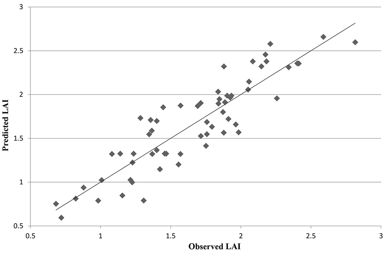
Fig. 3 - Residuals vs. fitted LAI values, generated with the MLR 3 model on Sentinel 2 and ALOS2 inputs, with R2 equal to 0.84 and according to the following equation: LAI = 3.133 - 6.00 B4 + 0.769 ARVI + 0.0820 HV.
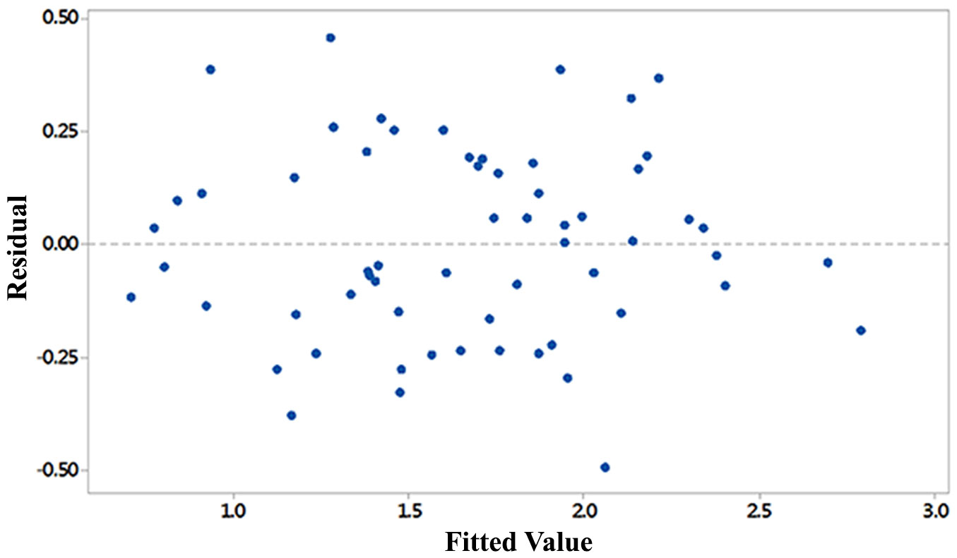
Fig. 4 - Map of the Leaf Area Index in the study area, based on Sentinel 2 and ALOS 2 data, using MLR model.
Discussion
This research illustrates how to accurately estimate LAI in the Zagros protected forest based on satellite and field data.
Using Sentinel 2 inputs, the accuracy (R2) of LAI estimates resulted equal to 0.77 (with PLSR, based on 32 inputs) and 0.81 (with MLR, based on two stepwise selected inputs), respectively. Both these results are higher with respect to values obtained by Stenberg et al. ([43]), who used Landsat ETM data in conifer forests (R2 equal to 0.63); by Zhang et al. ([51]), who used IRS P6 LISS 3 imagery in a bamboo forest (R2 equal to 0.68); and by Korhonen et al. ([27]), who used Sentinel 2 in boreal forests (R2 equal to 0.73). On the other hand, the results of the present study are slightly less accurate than those obtained by Chen et al. ([7]), who used AVNIR 2 optical data in a mixed forest mountain area (R2 equal to 0.93), with higher values possibly thanks to the higher spatial resolution of AVNIR 2 with respect to Sentinel 2.
Sentinel 2 data are free of cost and have a very high revisiting time: the present research shows that this sensor can be an optimal choice for LAI estimation in a Mediterranean forest type. Band 4 (red band) and the ARVI vegetation index were the best predictors. Band 4 is linked to chlorophyll absorption, and thus to foliage density, and a recent study showed that this band can outperform other vegetation indices for LAI estimation ([21]). ARVI, based on a combination of blue and red channels, has a dynamic range similar to that of NDVI, but it resists atmospheric effects via a self-correction process, making it a useful index in most remote-sensing applications ([26]).
The accuracy of LAI estimates obtained with SAR data were lower than those obtained with multispectral data; the R2 was equal to 0.61 when all available SAR predictors (10) were used as input in the PLSR model, and to 0.71 when the ALOS HV channel - selected by stepwise regression - was used as input in the MLR model. The sensitivity to LAI of an HV cross-polarized signal is already known ([24]); the present research shows that the use of SAR can be a valid alternative to multispectral data in the case of cloud coverage.
The longer wavelength of ALOS2, compared to S1, explains the complete exclusion of the latter dataset from the selection operated by stepwise regression. In fact, ALOS2 L-band data better penetrate the canopy and report information on vegetation density, with respect to C-band data ([5]). Chen et al. ([7]) obtained results similar to those presented here using ALOS PALSAR to estimate forest LAI (R2 = 0.69), though no cross validation was performed in that study. Manninen et al. ([32]) using ENVISAT ASAR data obtained results in the same range of accuracy (R2 = 0.69) in boreal forests. Higher accuracy in the LAI estimate (R2 = 0.79) was obtained by Kovacs et al. ([28]) using full-pol ALOS PALSAR data, characterized by four polarization channels and thus a higher information content.
The most accurate model was obtained integrating SAR ALOS 2 and multispectral S2 data: using MLR algorithm an accuracy (R2) equal to 0.84 was obtained. This result confirms the advantage, for the extraction of biophysical parameters in forests, of joining different datasets coming from complementary portions of the electromagnetic spectrum as previously observed by other authors ([46]). It is also worth noting that L-band data are scarcely influenced by the phenological stages of trees, as at this wavelength the signal is mainly influenced by the forest volume and the water content, thus allowing an easier comparison of LAI estimates carried out on different dates.
To conclude, the use of advanced algorithms such as RF or PLSR did not increase the accuracy of the LAI estimates with respect to MLR, possibly due to the clear linearity of the relationships. However, the use of MLR required a preliminary selection of predictors by stepwise regression, to prevent multicollinearity. To simplify the analysis, the PLSR algorithm is suggested as it can manage a large number of predictors; in this research, PLRS generated LAI estimates characterized by high accuracy (R2 = 0.80), in a range of values similar to those produced using MLR.
Author’s contribution
Conception or design of the work: SV; methodology development: SV, OF, GVL; data collection: SV, OF, HF; data analysis and interpretation: SV, GVL, NP; drafting the article: SV, OF, SR; critical revision of the article: GVL.
Acknowledgments
This research was funded with the contribution of the Italian Ministry of Agricultural, Food, and Forestry Policies (MiPAAF) subproject “Precision Forestry” (AgriDigit program - DM 36503.7305.2018 of December 2, 2018).
References
Gscholar
Gscholar
CrossRef | Gscholar
Online | Gscholar
Gscholar
Online | Gscholar
CrossRef | Gscholar
CrossRef | Gscholar
Supplementary Material
Authors’ Info
Authors’ Affiliation
Faculty of Agriculture and Natural Resources, Lorestan University, Khorramabad, Lorestan (Iran)
Department of Forestry, Ahar Faculty of Agriculture and Natural Resources, University of Tabriz (Iran)
Gaia Vaglio Laurin 0000-0002-6728-3557
Research Centre for Forestry and Woodland, Council for Agricultural Research and Economics, Arezzo (Italy)
Department of Geography, Amin Police University, Tehran (Iran)
Department of Forestry, Faculty of Natural Resources, University of Guilan, Someh Sara (Iraq)
Department for Innovation in Biological, Agro-food and Forest systems, Tuscia University, Viterbo (Italy)
Corresponding author
Paper Info
Citation
Vafaei S, Fathizadeh O, Puletti N, Fadaei H, Baqer Rasooli S, Vaglio Laurin G (2021). Estimation of forest leaf area index using satellite multispectral and synthetic aperture radar data in Iran. iForest 14: 278-284. - doi: 10.3832/ifor3633-014
Academic Editor
Agostino Ferrara
Paper history
Received: Aug 24, 2020
Accepted: Apr 08, 2021
First online: May 29, 2021
Publication Date: Jun 30, 2021
Publication Time: 1.70 months
Copyright Information
© SISEF - The Italian Society of Silviculture and Forest Ecology 2021
Open Access
This article is distributed under the terms of the Creative Commons Attribution-Non Commercial 4.0 International (https://creativecommons.org/licenses/by-nc/4.0/), which permits unrestricted use, distribution, and reproduction in any medium, provided you give appropriate credit to the original author(s) and the source, provide a link to the Creative Commons license, and indicate if changes were made.

Web Metrics
Breakdown by View Type
Article Usage
Total Article Views: 42864
(from publication date up to now)
Breakdown by View Type
HTML Page Views: 34793
Abstract Page Views: 4206
PDF Downloads: 3182
Citation/Reference Downloads: 10
XML Downloads: 673
Web Metrics
Days since publication: 1842
Overall contacts: 42864
Avg. contacts per week: 162.89
Article Citations
Article citations are based on data periodically collected from the Clarivate Web of Science web site
(last update: Mar 2025)
Total number of cites (since 2021): 3
Average cites per year: 0.60
Publication Metrics
by Dimensions ©
Articles citing this article
List of the papers citing this article based on CrossRef Cited-by.
Related Contents
iForest Similar Articles
Research Articles
Mapping Leaf Area Index in subtropical upland ecosystems using RapidEye imagery and the randomForest algorithm
vol. 7, pp. 1-11 (online: 07 October 2013)
Review Papers
Remote sensing-supported vegetation parameters for regional climate models: a brief review
vol. 3, pp. 98-101 (online: 15 July 2010)
Review Papers
Remote sensing of selective logging in tropical forests: current state and future directions
vol. 13, pp. 286-300 (online: 10 July 2020)
Research Articles
Estimation of forest cover change using Sentinel-2 multi-spectral imagery in Georgia (the Caucasus)
vol. 13, pp. 329-335 (online: 07 August 2020)
Research Articles
Assessing the influence of different Synthetic Aperture Radar parameters and Digital Elevation Model layers combined with optical data on the identification of argan forest in Essaouira region, Morocco
vol. 17, pp. 100-108 (online: 24 April 2024)
Review Papers
Accuracy of determining specific parameters of the urban forest using remote sensing
vol. 12, pp. 498-510 (online: 02 December 2019)
Research Articles
Afforestation monitoring through automatic analysis of 36-years Landsat Best Available Composites
vol. 15, pp. 220-228 (online: 12 July 2022)
Technical Reports
Detecting tree water deficit by very low altitude remote sensing
vol. 10, pp. 215-219 (online: 11 February 2017)
Review Papers
Remote sensing support for post fire forest management
vol. 1, pp. 6-12 (online: 28 February 2008)
Research Articles
Remote sensing of Japanese beech forest decline using an improved Temperature Vegetation Dryness Index (iTVDI)
vol. 4, pp. 195-199 (online: 03 November 2011)
iForest Database Search
Search By Author
Search By Keyword
Google Scholar Search
Citing Articles
Search By Author
Search By Keywords
PubMed Search
Search By Author
Search By Keyword


