Estimation of forest cover change using Sentinel-2 multi-spectral imagery in Georgia (the Caucasus)
iForest - Biogeosciences and Forestry, Volume 13, Issue 4, Pages 329-335 (2020)
doi: https://doi.org/10.3832/ifor3386-013
Published: Aug 07, 2020 - Copyright © 2020 SISEF
Research Articles
Abstract
Our objective was to use Sentinel-2A multispectral data in order to cost-effectively detect change in forest cover in Georgia (the Caucasus). Generalized additive models (GAMs) were used to fit forest cover measures to Sentinel-2A spectral band values modified using different topographic correction methods. Canopy closure (calculated from upward-looking fisheye photographs taken beneath forest canopy) was the best forest cover measure accounted for by the Sentinel-2 spectral data that were topographically corrected using the Minnaert Correction (R2 = 0.882). Spectral bands best explaining canopy closure were Band 3 (Green), Band 8 (NIR) and Band 12 (SWIR). Our model is able to reasonably detect spatial and temporal changes in canopy closure, even in highly rugged terrain and diverse vegetation cover, and it has potential to be improved to the extent that it can be applied by managers of natural resources. Based on free open source applications in combination with cheap gadgets our approach might play an important role in monitoring the forests of countries with low economic indicators.
Keywords
Generalized Additive Models, Forest Cover, Satellite Imagery, Sentinel-2, Fisheye, Topographic Correction
Introduction
Forest degradation caused by processes such as illegal logging, forest fires, and diseases is a widespread problem. Deforestation aggravates soil erosion, which in turn can have an irreversible effect on forest structure. Forest losses are due to various factors, such as forestry operations, land use changes, forest fires, and urbanization ([9]). Forest disturbance in the Caucasus is caused by selective logging rather than clear-cutting or other anthropogenic factors. Clear-cutting, more so than selective logging, adversely affects the integrity of the forest ecosystem; damage is caused to the remaining trees, soil, water balance, carbon accumulation and biodiversity ([2]).
Identifying disturbances in forest cover for large areas is an important task not only to study forest ecosystems but also to monitor anthropogenic impacts. Today remote sensing is the most practical and accurate tool for determining changes in forest cover at the regional level ([3]). With the development of satellite technology, the quality of mapping of forest canopy cover and the detection of deforestation and forest disturbance has significantly improved ([1]). Free remote sensing data (e.g., Landsat, MODIS, Sentinel) makes it possible to create monitoring systems of regional or planetary scales. At present global forest monitoring systems are mainly based on 30-meter resolution data from Landsat satellites ([3], [19], [20]).
Changes in forest cover are not always distinguished by modern monitoring systems based on remote sensing data. The fact is that in global models it is not always possible to distinguish forest degradation because the density and structure of trees are difficult to interpret in satellite images of medium resolution ([25]). Difficulties also arise with the use of topographic image correction in rugged terrain because of topographic illumination effects ([27], [36]). Because topographic effects may have dramatic impacts on the outcomes of time series and change detection studies, topographic correction of remotely sensed imagery over mountainous regions in these studies is critical ([27]). Also, the limitation in the interpretation of the forest arises due to its vertical structure, as it is extremely complicated to detect degradation under the closed canopy cover using optical satellites ([25]). The accuracy of the models also depends on the capabilities of the satellite data. For example, Sentinel-2 provides better models of forest cover (CC), effective cover (ECC) and leaf area index (LAI) in lowland boreal forests than Landsat 8 ([24]).
Mapping of forest cover using remote sensing is usually performed by land classification into forest and non-forest. However, the maps derived from satellite data depend on the definition of the forest, mainly on the threshold of tree cover parameters, above which the territory is identified as a forest ([34]). An alternative approach is continuous surface that can represent areas of heterogeneous tree cover better than models based on discrete interpretation ([18]). To assess the ecological characteristics of the forest, canopy closure is one of the most useful determinants of its structure and biophysical attributes such as tree density and health ([6]). Canopy closure is also an important measure to estimate the distribution of trees on a global scale ([8]). Hemispherical photography is one of the many ways to measure canopy closure and obtain various biophysical parameters ([11], [5]). Models of solar radiation transmittance through the canopy are widely used in remote sensing ([33]) as the canopy structure provides important information on the functions and dynamics of the forest ecosystem ([4]). Although there have been many studies of calibrating forest cover parameters (including canopy closure, LAI) against remotely sensed spectral bands and vegetation indices derived from these bands, a set of spectral predictors for each of the forest cover parameters substantially varies with sensors, forest structure and geography ([29]).
In this study we used digital hemispherical photography in combination with remote sensing for the first time in the Caucasus. The main goal of this study was to evaluate the possibility of creating a forest monitoring system based on freely available software and satellite multispectral images of Sentinel-2 for heterogeneous and rugged areas of Georgia and Caucasus. More specifically we attempt to find a quantitative indicator of forest cover that can be best explained temporally and spatially by the Sentinel-2 multispectral bands through testing various topographic correction methods. Maps derived from our model will help efficiently monitor land surface change, especially that of forest cover.
Materials and methods
Study area and sampling
Our objective was to use Sentinel-2A multispectral data in order to detect change in forest cover. To maximize statistical representativeness of our sample (i.e., variability of response and explanatory variables) we sampled old-growth forests, the tree line (i.e., the elevation above which trees fail to grow), forests with logging operations and ecological succession processes. We conducted our fieldwork in 2018 between July 7 and August 15 in two regions: Central Georgia including coniferous and mixed forests and Eastern Georgia including deciduous forests (Fig. 1). Forest cover parameters (Tab. S1 in Supplementary material) were measured within 20 × 20 m plots whose sides were oriented parallel to the true north-south axis. The plots were distributed evenly across 4 categories of tree cover percentage: 0-25%, 25-50%, 50-75%, 75-100%. The tree cover percentage was estimated visually by two foresters on the field.
Fig. 1 - Sampling plots for forest cover parameters and the extents of two Sentinel images intersecting Central Georgia (at left) and Eastern Georgia. The map is projected to UTM Zone 38N; WGS: 1984.
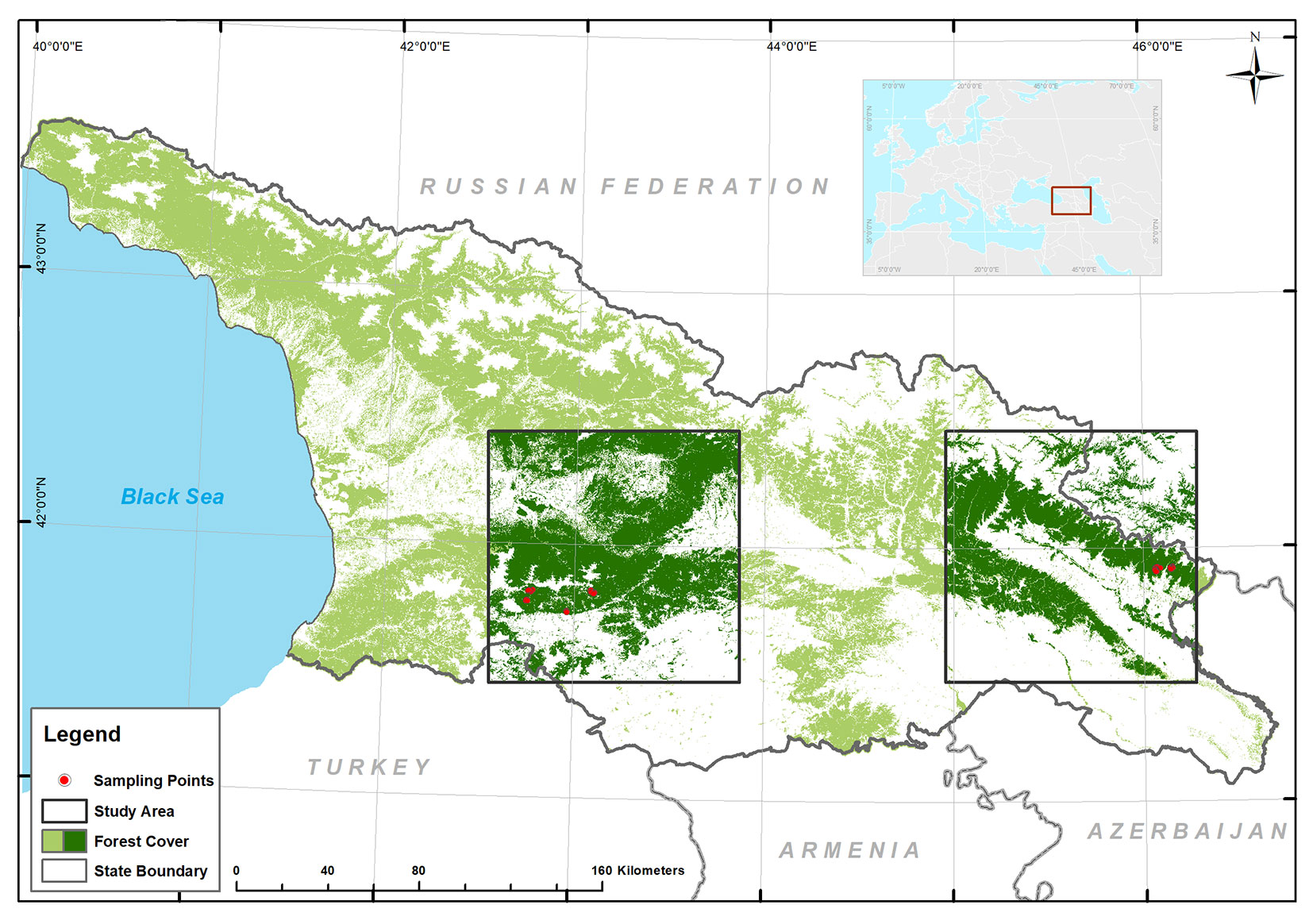
During the most stable vegetation period from July to early September, we were able to process a total of 80 plots: 45 plots in Central Georgia and 35 plots in Eastern Georgia (Fig. 1). More specifically, 20 plots at Otskhora, 5 plots at Kurtskhana (tributaries of Abastumani River), 5 plots at Tsveruknis Ghele, 15 plots at Bagebis Ghele (tributaries of Mtkvari River) and 35 plots at Kabali River (a tributary of Alazani River). The plots were dominated by any of the following species: Abies nordmaniana, Picea orientalis, Pinus kochiana, Carpinus betulus, Fagus orientalis, Quercus iberica, Dryopteris filix mas, Festuca sp., Rubus caucasicus, and a plant community of subalpine meadows (a mixture of grassland, Rhododendron caucasicum and stunted Betula spp.). The species dominance in the plot was assigned by either the tree basal area or the percent vegetation cover: the tree species, whose basal area was the largest in a plot, was considered as dominant in the plot, while in a tree-less plot the plant species or community that had the largest percent cover, was considered as dominant.
Forest cover parameters
The ratio of the area of canopy to the sky was measured using a mobile phone (Huawei P9®, 12MP) with AMIR photo 180° Fisheye Lens and the software Gap Light Analyzer 2.0 ([12]). The hemispherical images were taken in the center of the study plot, normal to the horizontal (i.e., photographs oriented parallel to the horizontal) at a height of 30 cm above ground under the diffuse sky (i.e., uniformly overcast sky, or sky near sunrise or sunset). All images containing such obstructing objects as boulders, cliffs, fallen trees or hills and peaks were excluded from further processing. The field of view of each image was reduced to 90o in order to (i) reduce distortions and noise near the edge and (ii) remove shaded fractions introduced by the steepest (i.e., 38o) of the slopes in our data set. The blue channel of each image, which maximizes the contrast between sky and canopy, was chosen. Then the separation of pixels within each image into sky and non-sky classes was performed by visually (i.e., subjectively) selecting a threshold value for each hemispherical image, which best separated the sky pixel from canopy. Lastly, the proportion of canopy pixels was computed for each image (hereafter the canopy closure). This entire procedure was performed separately by three image interpreters, and the mean of the three canopy closure values was used for each of the images.
The tree diameter and basal area was measured at 1.3 m above ground, at the breast height (DBH), using forestry caliper (Nestle forestry caliper Waldmeister, Dornstetten, Germany). Individual basal areas were summarized to calculate the total basal area of a study plot. The tree height was measured using Suunto PM5/SPC® Clinometer (Vantaa, Finland) and averaged in a study plot.
Satellite imagery
For remotely sensed spectral data we used the already orthorectified Sentinel-2A imagery (available at ⇒ https://scihub.copernicus.eu/dhus/#/home), which consists of 13 bands with three different resolutions (10, 20 and 60 m). Because of extensive cloudiness in the sentinel imagery for our entire study period we had to use two scenes: one acquired on July 1, 2018 for Eastern Georgia and the other one acquired on August 28, 2018 for Central Georgia. Due to the limited availability of cloud-free imagery difference in time between sampling forest cover parameters and Sentinel image acquisition varied between 6 and 45 days (mean ± SD = 25.225 ± 13.153). The sampled and spectral data (Tab. S1 in Supplementary material) were mapped and organized into a data frame using QGIS Desktop 3.4.5-Madeira software package ([31]).
Most of the territory of Georgia, including our study area, is substantially rugged, which greatly affects the interpretability of satellite images. Therefore, in addition to atmospheric correction, we also applied topographic correction. Sen2Cor, which is a processor for Sentinel-2 Level 2A product generation and formatting, was used to perform atmospheric and cirrus correction of Top-Of-Atmosphere Level 1C input data. Bottom-Of-Atmosphere Level 2A reflectance images were created using the following parameters: solar zenith angle, sensor view angle, relative azimuth angle, ground elevation, visibility and water vapor. All parameter values were derived from image metadata. Four topographic correction methods were tested: (i) topographic effect correction through the Sen2cor radiometric correction processor (hereafter, Sen2cor-corrected Sentinel bands); (ii) the Cosine Correction (hereafter C-corrected Sentinel bands - [37]); (iii) the Minnaert Correction (hereafter M-corrected Sentinel bands - [35], [13]); and (iv) the Normalization Method (hereafter N-corrected Sentinel bands - [7]). For data processing we used SAGA-System for Automated Geoscientific Analyses. The most accurate effect of topographic correction is reached when using DEM and multispectral imagery at the same resolution ([22], [16]), we used SRTM with 30 m grid size, available from USGS data portals. Unfortunately, a more detailed DEM was not available in our study to match with 10-m and 20-m spatial resolutions of our spectral data. The selected SRTM30 DEM for the study area was downloaded from free data portals (source: United States Geological Surveys - ⇒ https://earthexplorer.usgs.gov/). The DEM contained errors in the form of spikes and gaps (elevation data outliers). For correction, we applied a 3 × 3 median filter using SAGA tools.
Model development
Generalized additive models (GAMs) were used to fit forest cover parameters to Sentinel-2A spectral band values using the “mgcv” package ([43]) in R version 3.5.2 ([32]). The possible effects of difference in time between sampling forest cover parameters and Sentinel image acquisition were also estimated. We used GAMs because without any assumptions they are able to find nonlinear and non-monotonic relationships, and have been successfully used in satellite-based canopy cover estimation ([17]). GAMs were fitted using a Gamma family with a log link function, a Gaussian family with an identity link function and a binomial family with a logit link function. The binomial family was used for proportion response variables. Penalized thin plate regression splines were used to represent all the smooth terms. The restricted maximum likelihood (REML) estimation method was implemented to estimate the smoothing parameter because it is the most robust of the available GAM methods ([43]).
Model and variable selection were performed by exploring all possible subsets of predictor variables, where pairwise correlations between variables were less than 0.9. To get subsets of predictor variables, thousands of variable combinations were generated using the “gtools” package for R ([40]). The predictive power of the models was evaluated through a leave-one-out cross-validation. The cross-validation of thousands of models was handled through R’s parallelization capabilities ([41], [42]). The best models were selected by the mean squared error. We also checked concurvity between model terms and between each term and the rest of the model using the “mgcv” package. Akaike’s Information Criterion (AIC) is generally used as a means for model selection. However, we preferred cross-validation for model selection because AIC a priori assumes that simpler models with the high goodness of fit are more likely to have the higher predictive power, while cross-validation without any a priori assumptions measures the predictive performance of a model by efficiently running model training and testing on the available data.
All gridded predictor layers (raster layers) were resampled to a resolution of 10 m using the nearest-neighbor assignment technique of QGIS Desktop 3.4.5-Madeira. The best forest cover model was predicted to the raster layers using the raster package ([21]) in R version 3.5.2. To produce the final maps, the gridded estimates of the best forest cover parameter and their standard errors were masked with the forest cover developed for National Forest Agency (NFA) in 2015-2016. The NFA forest cover is defined as a grid of 0.5 ha cells where crown cover is > 20%.
From gridded estimates and standard errors, we derived statistically significant differences in forest cover (p-value < 0.05) between July 1, 2018 and August 5, 2016 and between August 28, 2018 and August 14, 2015 for the Sentinel-2A scenes of Eastern Georgia and Central Georgia, respectively. Appendix 1 in Supplementary material contains the main R codes and the data set used in this study.
Model validation
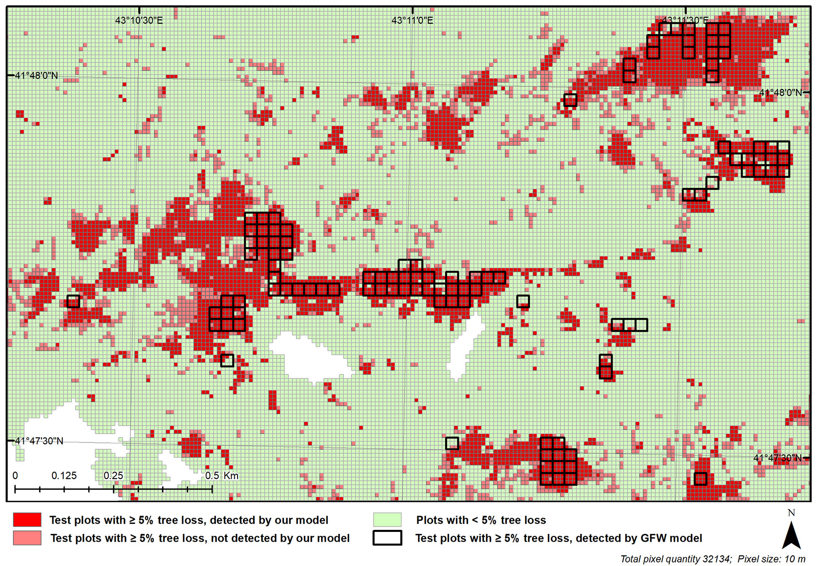
Finally, we tested and compared the accuracy of detecting tree loss between our model and the maps produced by Global Forest Watch (GFW - ⇒ http://www.globalforestwatch.org/map). To do so, we used a 1.38 × 2.44 km grid of 10 × 10 meter plots that were classified into those where percentage of tree loss from 2016 through 2017 was ≥ 5% and those where the loss percentage was less (source: Agency of protected area). There were 6032 plots with ≥ 5% tree loss (hereafter test plots) in this grid that covered an area located in Borjom-Kharagauli National Park (Central Georgia). Based on loss of tree cover on the GFW maps and statistically significant loss in forest cover of our model, we checked what portion of the test plots was detected by our and GFW models. We used this qualitative approach because a relevant quantitative measure of forest cover in the test area was not available to test our model. The altitudinal range of the test plots were from 1256 to 2113 m a.s.l. (mean ± SD = 1613 ± 162), while their slope range in degrees varied from 0 to 67.1 (mean ± SD = 28.2 ± 8.0). Tree density in these plots varied from 0 to 0.8 (mean ± SD = 0.44 ± 0.32). Canopy structure, vegetation types and diversity were much the same as in the training plots.
Results
Based on the exhaustive cross-validation procedure GAMs fitted to the canopy closure performed much better than those fitted to the other forest cover parameters (i.e., tree cover percentage defined by foresters on the field, total basal area, and tree average height). No more than 70% in the variation of the other forest cover measures could be explained by GAMs (Tab. S2 in Supplementary material). The best model of the canopy closure was the one that was fitted to M-corrected three spectral bands using a binomial family with a logit link function for proportion data (Tab. 1, Tab. 2, Fig. 2, Fig. 3 - see also Fig. S1 and Fig. S2 in Supplementary material). In addition to the lowest cross-validation error, the relationship between the canopy closure and the M-corrected three spectral bands had the greatest goodness of fit, the least complexity and the shortest residual range.
Tab. 1 - The diagnostics of the canopy closure models derived through different topographic corrections of Sentinel-2 bands. (MSE): Mean squared error; (Dev. Expl.): explained deviance; (AIC): Akaike’s Information Criterion; (df): degrees of freedom.
| Topographic correction |
Cross-validation MSE |
100% range limits of residuals |
95% range limits of residuals |
R2adj | Dev. Expl. (%) |
AIC | df |
|---|---|---|---|---|---|---|---|
| Sen2cor | 279.332 | -35.676 - 17.838 | -20.073 - 13.533 | 0.864 | 88.6 | 4119.893 | 26.078 |
| Cosine | 258.328 | -35.274 - 36.425 | -15.830 - 22.141 | 0.819 | 84.7 | 5366.458 | 26.133 |
| Minnaert | 178.620 | -24.894 - 14.952 | -16.973 - 14.358 | 0.882 | 89.8 | 3736.264 | 25.351 |
| Normalization Method | 232.788 | -33.086 - 38.060 | -23.560 - 16.510 | 0.815 | 83.5 | 5734.853 | 25.935 |
Tab. 2 - Summary of the generalized additive model (GAM) analysis for modeling the canopy closure (FEYE) as forest cover measure fit to Sentinel-2A spectral band values. (n): sample size; (s()): spline smooth function; (edf): estimated degrees of freedom; (P): significance of terms. See Tab. S1 in Supplementary material for the description of variables.
| n | Variable term | edf | P | Goodness of fit (R2adj) |
Deviance explained |
|---|---|---|---|---|---|
| 80 | s(B03) | 8.106 | <2e-16 | 0.882 | 89.8 % |
| s(B08) | 7.845 | <2e-16 | |||
| s(B12) | 8.033 | <2e-16 | |||
| Intercept = -16.477 | - | 0.00106 |
Fig. 2 - GAM-fitted relationships of the canopy closure (FEYE) in fractions and Sentinel-2A spectral bands in reflectance values ×10.000. Band suffix M18 stands for M-corrected band acquired in 2018.
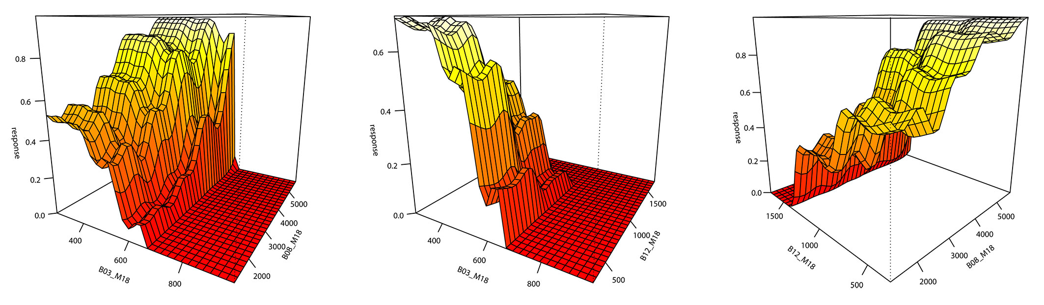
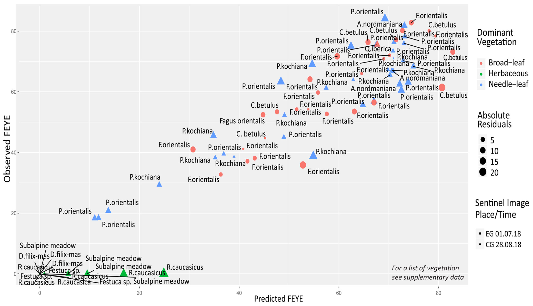
Fig. 3 - Scatter plot of fitted and observed FEYE values: the canopy closure (FEYE) GAM-fitted to M-corrected reflectance values of Sentinel-2A, using the REML smoothing parameter estimation (adjusted R2=0.882). Graph points, labeled with dominant plant species, represent study plots whose color, size and shape indicate dominant vegetation cover, absolute residuals and Sentinel image acquisition place-date, respectively. The tree species, whose basal area is the largest in a plot, is considered as dominant in the plot, while in a tree-less plot the plant species or community, that has the largest percent cover, is considered as dominant.
Each of the four topographic correction methods suggested the same set of three bands best explaining variation in the canopy closure. These were Band 3 (Green), Band 8 (NIR) and Band 12 (SWIR). Band 8 was generally positively correlated with the canopy closure, while Band 3 and 12 were generally negatively correlated (Fig. 2). The magnitude of model fit for topographic correction in decreasing order was as follows.
Absolute difference in time between sampling forest cover parameters and Sentinel image acquisition did not have a considerable effect on absolute values of residuals (R2 = 0.0022, adjusted R2 = -0.01061, p-value = 0.68). Difference in location and timing between the two scenes also did not have effect on the model. Some land surface features such as high cornfields, deep water bodies, some wetlands and orchards showed FEYE as high as forests (up to 80%). However, these features were masked out by the NFA forest cover. Our model detected true changes where forest damage was caused by selective cutting, clear-cutting, pest outbreak, and forest fires while canopy closure gain was caused by some agricultural operations such as the cultivation of hazelnuts and orchards (Fig. S3, Fig. S4). Our model detected 61.3% of the test plots, while that of GFW detected 14.8% of the test points (Fig. 4). Tab. S3 in Supplementary material contains gridded estimates of and changes in canopy closure during the study period throughout the country of Georgia.
Fig. 4 - Testing the model accuracy of detecting tree loss from 2016 through 2017 in Borjom-Kharagauli National Park (Central Georgia). The map is projected to UTM Zone 38N; WGS: 1984.
Discussion
In our study, the magnitude of the canopy closure was the best forest cover measure accounted for by the Sentinel-2 spectral data that were topographically corrected using the Minnaert Correction. Spectral bands best explaining the canopy closure were Band 3 (Green), Band 8 (NIR) and Band 12 (SWIR).
The best performance of the canopy closure in relation to satellite spectral data was expected because fisheye photographs rather than the other tree stand parameters show how much light per area is reflected and absorbed by vegetation cover. We tested 67 spectral predictors (10 Sentinel bands and 57 vegetation indices derived from these bands - Tab. S1 in Supplementary material). Out of these 67 predictors our cross-validation procedure suggested that only the three were sufficient to account quite accurately for changes in canopy closure. The importance of NIR and SWIR was not surprising because NIR and SWIR are widely used to estimate green biomass and detect changes in vegetation density. In agreement with our findings SWIR, in contrast to NIR, was shown to have lower values for larger canopy closure and greater vegetation density ([14], [23], [26], [30]). As for the negative response of the canopy closure to Band 3 (Green) other studies also showed that green biomass had the strongest negative correlation with reflectance in the green band of all visible wavebands ([28]). Umarhadi et al. ([39]) also found the negative correlation between Sentinel B3 and canopy closure measured using hemispherical photography. The green band might also act as a variable that best minimizes shade fraction or saturation effects on NIR and SWIR. The vegetation indices, especially NDVI, performed poorly probably because they asymptotically approach the saturation in dense vegetation or high canopy regions ([38], [15]). Sentinel-2 imagery topographically processed through the Minnaert Correction resulted in more accurate models than those based on the Cosine Correction, the Normalization method and the Sen2cor-correction. This is in agreement with some other studies ([10]).
Our GAM-fitted canopy closure model predicts much higher values than the observed ones for some areas, where there are few or no trees. This is probably due to the fact that we underestimated the light-absorbing power of some non-tree low vegetation such as Rubus caucasicus and subalpine meadows sparsely scattered with low birch trees. Most of our model errors are probably accounted for by the coarser DEM being used to minimize topographic effects on Sentinel-2 spectral reflectance values.
Some land surface features (e.g., high corn fields, deep water bodies, some wetlands mostly dominated by Carex spp. and orchards) showed fisheye values as high as forests (up to 80%). This error is especially noticeable on the northern slopes of alpine meadows where Rhododendron caucasicum and stunted birch trees are distributed. This is because (i) some of these cover types are dense and tall enough to have a large shade fraction or (ii) their spectral signatures were not covered in our sample. However, these problematic features were masked out by the NFA forest cover. We also noticed that the models of topographic correction tested have a different impact on forest types, for example, in more rugged areas the canopy closure of deciduous trees was better explained than that of coniferous trees. Perhaps, steep slopes with dark coniferous trees darken the area on the image, which, in turn, distorts the process of topographic normalization. Sentinel-2 acquisition date and place, as well as difference in time between sampling tree stand parameters and Sentinel image acquisition, did not have a considerable effect on model accuracy; that makes our model reasonably robust. Although our model of loss/gain of canopy closure in the forest has reasonable predictive power, this study raises questions related to the improvement of methods for topographic correction for highly rugged terrain with regard to classifying and quantifying vegetation cover.
Our model performed much better on the test points than that of GFW. Our model detected 61.3% of the test plots, which is not as high as we expected. However, this can be explained by the fact that the test plots were identified using the number of trees removed from the plot whereas our model is actually designed to measure canopy closure that is a function of not only the number of trees, but also their sizes and taxonomic identity. GFW is an online near real-time monitoring and alert system, which uses Landsat imagery and powerful computational resources to detect annual changes in forest cover at the planetary scale. However, despite the impressive results of the determination of annual changes in forests, the GFW has a limitation associated with the spatial resolution of the Landsat imagery. The loss of tree cover on GFW maps shows the complete removal of a canopy of tree cover at a resolution of 30 × 30 meters (GFW - [20]) which is not enough to monitor forests where degradation is mainly caused by selective logging or other changes at a finer scale.
Conclusion
As far as we know, this is the only model of tree loss and gain obtained through a cost-effective approach to the exhaustive analysis of reflectances and many indices that were derived from Sentinel-2 data. Cost-effective approaches in the future should play an important role in monitoring the forests of countries with low economic indicators. There are quite a few models specifically designed to assess the loss of trees and forest degradation. There are also many instruments and methodologies for measuring forest structures and parameters, but they are not always cost-effective since the development of a monitoring system can be costly. Our main goal was to test the possibility of creating a system for detecting the loss of forest cover in highly rugged terrain and diverse vegetation cover of the Caucasus based on free Sentinel-2 satellite data and free software applications. For field work, we used the simplest devices, including non-professional “fisheye” lenses for mobile phones. The sample size was also minimal. We believe that models created using open source applications in combination with cheap gadgets in the future will change the rules of the game and greatly facilitate the assessment and management of natural resources. We think our model is able to reasonably detect spatial and temporal changes in forest cover, and it has potential to be improved to the extent that it can be applied by managers of natural resources in particular by wildlife managing and forestry agencies.
Acknowledgements
We would like to thank Alexander Giorgadze, David Gelashvili, Giorgi Janashvili for helping during field measurements and Nutsa Megvinetukhutsesi for assisting in mapping. Financial support was provided by World Resources Institute in the framework of Global Forest Watch, and by UNEP/ GEF. We would also like to acknowledge the useful comments and suggestions of two anonymous reviewers.
Declaration of interest
The authors certify that they have no affiliations with or involvement in any organization or entity with any financial interest (such as honoraria; educational grants; participation in speakers’ bureaus; membership, employment, consultancies, stock ownership, or other equity interest; and expert testimony or patent-licensing arrangements), or non-financial interest (such as personal or professional relationships, affiliations, knowledge or beliefs) in the subject matter or materials discussed in this manuscript.
References
CrossRef | Gscholar
Gscholar
CrossRef | Gscholar
Gscholar
Online | Gscholar
CrossRef | Gscholar
Gscholar
Gscholar
CrossRef | Gscholar
Supplementary Material
Fig. S2 - The histogram of residuals of the canopy closure (FEYE) fitted to Sentinel reflectance values topographically corrected using Minnaert Correction.
Fig. S3 - Modeled canopy closure (FEYE) in eastern Georgia (at left) and statistically significant differences in the canopy closure in percentage at two sites between July 1, 2018 and August 5, 2016.
Fig. S4 - Modeled canopy closure (FEYE) in central Georgia (at left) and statistically significant differences in the canopy closure in percentage at two sites between Aug 28, 2018 and Aug 14, 2015.
Tab. S1 - List of the variables used for modeling forest cover.
Tab. S2 - The accuracy of the best fit GAM models for forest cover measures based on Minnaert-corrected Sentinel bands and family.
Appendix 1 - The main R codes used in the study.
Authors’ Info
Authors’ Affiliation
Alexander Gavashelishvili 0000-0001-9677-6038
Vasil Metreveli 0000-0002-9558-0655
Center of Biodiversity Studies, Institute of Ecology, Ilia State University, Cholokashvili Str. 5, 0162 Tbilisi (Georgia)
Department of Geoinformatics, Institute of Botany, Ilia State University, Botanical Str. 1, 0105 Tbilisi (Georgia)
Corresponding author
Paper Info
Citation
Mikeladze G, Gavashelishvili A, Akobia I, Metreveli V (2020). Estimation of forest cover change using Sentinel-2 multi-spectral imagery in Georgia (the Caucasus). iForest 13: 329-335. - doi: 10.3832/ifor3386-013
Academic Editor
Maurizio Marchi
Paper history
Received: Feb 25, 2020
Accepted: Jun 03, 2020
First online: Aug 07, 2020
Publication Date: Aug 31, 2020
Publication Time: 2.17 months
Copyright Information
© SISEF - The Italian Society of Silviculture and Forest Ecology 2020
Open Access
This article is distributed under the terms of the Creative Commons Attribution-Non Commercial 4.0 International (https://creativecommons.org/licenses/by-nc/4.0/), which permits unrestricted use, distribution, and reproduction in any medium, provided you give appropriate credit to the original author(s) and the source, provide a link to the Creative Commons license, and indicate if changes were made.

Web Metrics
Breakdown by View Type
Article Usage
Total Article Views: 47353
(from publication date up to now)
Breakdown by View Type
HTML Page Views: 38634
Abstract Page Views: 4394
PDF Downloads: 3487
Citation/Reference Downloads: 11
XML Downloads: 827
Web Metrics
Days since publication: 2179
Overall contacts: 47353
Avg. contacts per week: 152.12
Article Citations
Article citations are based on data periodically collected from the Clarivate Web of Science web site
(last update: Mar 2025)
Total number of cites (since 2020): 6
Average cites per year: 1.00
Publication Metrics
by Dimensions ©
Articles citing this article
List of the papers citing this article based on CrossRef Cited-by.
Related Contents
iForest Similar Articles
Review Papers
Remote sensing-supported vegetation parameters for regional climate models: a brief review
vol. 3, pp. 98-101 (online: 15 July 2010)
Review Papers
Accuracy of determining specific parameters of the urban forest using remote sensing
vol. 12, pp. 498-510 (online: 02 December 2019)
Research Articles
Mapping the vegetation and spatial dynamics of Sinharaja tropical rain forest incorporating NASA’s GEDI spaceborne LiDAR data and multispectral satellite images
vol. 18, pp. 45-53 (online: 01 April 2025)
Research Articles
Estimation of forest leaf area index using satellite multispectral and synthetic aperture radar data in Iran
vol. 14, pp. 278-284 (online: 29 May 2021)
Review Papers
Remote sensing support for post fire forest management
vol. 1, pp. 6-12 (online: 28 February 2008)
Research Articles
Estimates of selective logging impacts in tropical forest canopy cover using RapidEye imagery and field data
vol. 9, pp. 461-468 (online: 11 January 2016)
Research Articles
Assessing the influence of different Synthetic Aperture Radar parameters and Digital Elevation Model layers combined with optical data on the identification of argan forest in Essaouira region, Morocco
vol. 17, pp. 100-108 (online: 24 April 2024)
Research Articles
Estimating biomass of mixed and uneven-aged forests using spectral data and a hybrid model combining regression trees and linear models
vol. 9, pp. 226-234 (online: 21 September 2015)
Review Papers
Remote sensing of selective logging in tropical forests: current state and future directions
vol. 13, pp. 286-300 (online: 10 July 2020)
Technical Reports
Remote sensing of american maple in alluvial forests: a case study in an island complex of the Loire valley (France)
vol. 13, pp. 409-416 (online: 16 September 2020)
iForest Database Search
Search By Author
Search By Keyword
Google Scholar Search
Citing Articles
Search By Author
Search By Keywords
PubMed Search
Search By Author
Search By Keyword


