Mapping the vegetation and spatial dynamics of Sinharaja tropical rain forest incorporating NASA’s GEDI spaceborne LiDAR data and multispectral satellite images
iForest - Biogeosciences and Forestry, Volume 18, Issue 2, Pages 45-53 (2025)
doi: https://doi.org/10.3832/ifor4632-017
Published: Apr 01, 2025 - Copyright © 2025 SISEF
Research Articles
Abstract
This study integrates NASA’s Global Ecosystem Dynamics Investigation (GEDI) spaceborne LiDAR data with multispectral satellite imagery to map the vegetation and assess spatial dynamics within the Sinharaja Forest Reserve (SFR). Utilizing advanced remote sensing techniques, we delineated vegetation structure, vegetation density distribution, and canopy cover at high spatial resolutions. Eight distinct vegetation/land cover types were identified by this work and an updated vegetation map was developed for SFR. The resulted map recorded an estimated overall accuracy of 90% (Kappa coefficient 0.9) by the accuracy assessment. Comprehensive insights into forest composition and spatial dynamics were achieved with regard to canopy heights, plant area index and plant area volume density. Our results suggest that the integration of GEDI LiDAR and satellite imaging data offers a robust framework for characterizing tropical forest ecosystems, facilitating better understanding of their ecological processes, and informing conservation and management strategies.
Keywords
Forest Dynamics, Remote Sensing, Land Cover, Forest Ecology, Vegetation Density
Introduction
Tropical forests once covered 12 percent of Earth’s terrestrial surface and have now been reduced to less than five percent ([7], [25], [5]) indicating the level of exploitation and land cover change caused by the unprecedented human activities. Tropical rainforests are the most biodiverse and productive terrestrial ecosystems on Earth, providing numerous ecosystem services ([38]). Warm temperatures, constant sunlight throughout the year, high precipitation, and high biodiversity lead to complex forest structures with multiple layers and a high species density. These aspects of tropical forests make vegetation mapping significantly more challenging, mainly when traditional methods are employed. The availability of accurate and detailed vegetation maps is an essential requirement in modern ecological studies ([18], [26]), providing critical information for a variety of applications ranging from land management, detecting forest cover changes, understanding biodiversity patterns, carbon cycling, vegetation protection, restoration programs, and conservation planning ([17], [12], [48], [49], [29]). In this context, with the constant development and evolution of remote sensing technologies, the availability of large Earth Observation (EO) datasets plays a vital role in vegetation mapping for both present and future applications. The significant improvements in spectral, temporal, and spatial resolutions of satellite imagery (i.e., Landsat and Sentinel systems) ([50]) and availability of novel auxiliary data sets such as NASA’s Global Ecosystem Dynamics Investigation (GEDI) spaceborne Light Detection and Ranging (LiDAR) have opened new horizons in land cover (LC) mapping and investigating the structural dynamics of forests.
According to Tierney et al. ([45]) vegetation maps are based on two essential elements: a classification of vegetation and a spatial attribution of that classification. Hence, the vegetation mapping groups together similar plant communities into a simplified form depicting their arrangement pattern with spatial reference ([9]). Landsat and Sentinel satellite missions provide two of the most prominent currently available free datasets of multispectral satellite imagery. The newest Landsat 8/9 and Sentinel 2 satellite images offer reasonably high spatial (up to 10 m) and spectral resolution, with multiple bands. Therefore, many land cover (LC) and vegetation mapping studies have utilized these multispectral satellite images for classification purposes in recent years. Xie et al. ([49]) mentioned the importance of incorporating spatial-based variables into spectral features, which leads to improved classification accuracy, as indicated by Han et al. ([23]) and Li et al. ([28]). While spectral indices, such as Normalized Difference Vegetation Index (NDVI), are extensively used for forest classifications, the usage of auxiliary spatial data is not shared. According to Xie et al. ([49]), the use of the forest stand structure features supports the separation of different forest types based on the tree species composition, canopy height, crown size and shape, and tree density. The difficulties in obtaining such data over large areas, based on air LiDAR , limit the number of studies that have incorporated these two aspects into forest classification. However, with the availability of NASA’s GEDI data from spaceborne LiDAR sensors, which are explicitly designed to measure Earth’s surface structure, including detailed information about the 3D canopy structure of terrestrial vegetation, the opportunity is open to utilize this data for forest classification. GEDI data generated by the sensor onboard the International Space Station (ISS) are available from March 2019, allowing the derivation of vertically resolved information related to canopy height, density, and layering through full waveform sampling ([24], [34], [42]).
The tropical island of Sri Lanka had a considerable forest cover a few centuries ago, even when -many protected areas were legally not in existence. However, the drastic decline in forested areas of the island, which has occurred over the last two centuries, has resulted in the current forest cover being less than 22% ([13]). The highest level of forest exploitation has occurred in the wet zone of the island, primarily due to increased anthropogenic activities and human settlement. Less than 2.1% of the original wet zone lowland forests still remain, and they also occur as fragmented, degraded, and isolated patches ([27]). In this context, we focused this research on Sinharaja Forest Reserve (SFR), which can be considered as Sri Lanka’s largest, relatively undisturbed rainforest ([11], [22]). Although the first published mapping effort of the Sinharaja forest dates back to the comprehensive work by Baker ([3]), only a handful of detailed vegetation maps are available for the area. Updated maps with detailed vegetation and LC details at high resolution are scarce. There’s one study that has focused on mapping the carbon stock of SFR based on Landsat image analysis ([36]). Work by Madurapperuma & Kuruppuarachchi ([33]) and Samarasinghe et al. ([41]) have attempted to detect the LC changes of Sinharaja based on Landsat images focusing on spectral information. Additionally, Lockwood ([30]) has conducted a classification attempt based on Planet Dove imagery. Wijesinghe & De Brooke L ([47]) categorized the primary and secondary vegetation as unlogged and selectively logged habitats. However, a map to represent the two habitat types is not available. When spatial dynamics of wet zone forests are considered, several plot-based studies have been conducted in the past ([1], [6], [6], [39]). However, a remote sensing approach covering the whole of SFR is not available. This research gap necessitates the requirement of an updated vegetation map, and our research was conducted with the objectives of developing a detailed vegetation map for SFR and utilizing modern remote sensing techniques to investigate the spatial dynamics of SFR vegetation structure.
Materials and methods
Study area
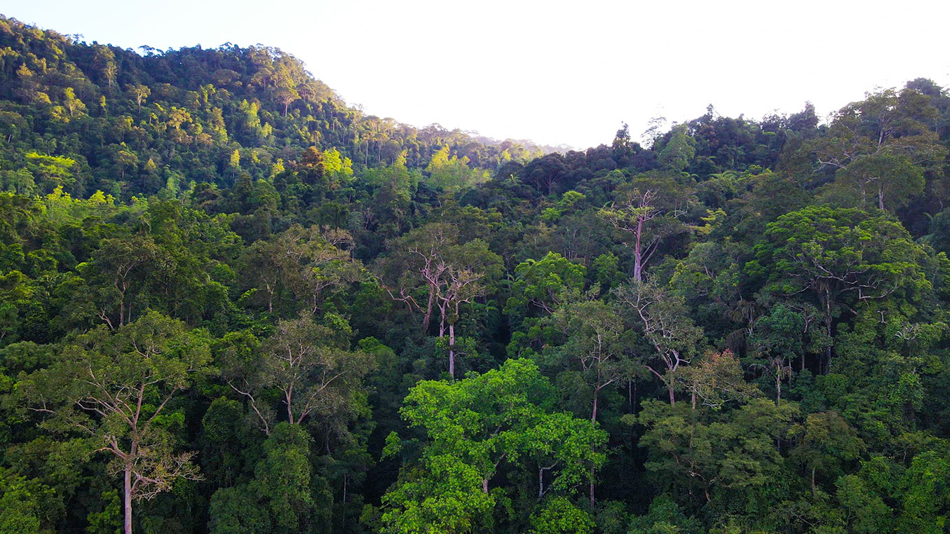
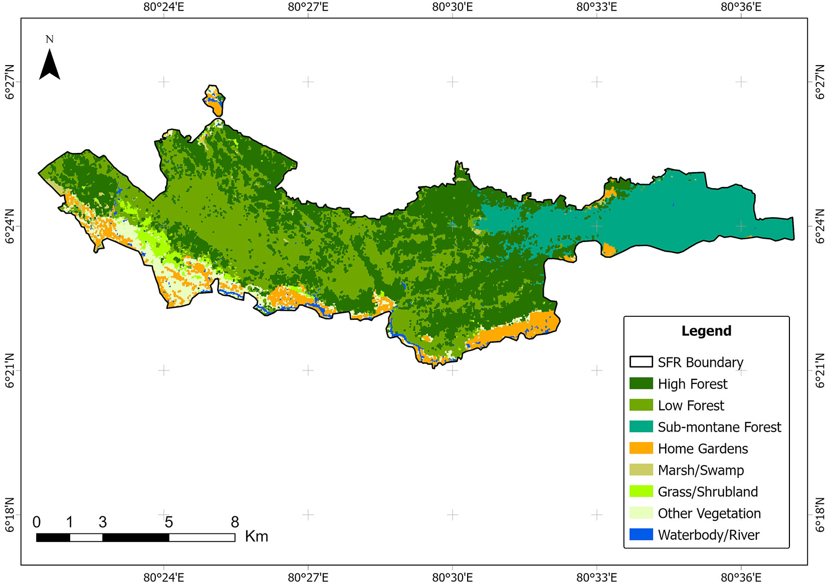
The study was conducted in Sinharaja Forest Reserve (SFR - Fig. 1) which is also a UNESCO World Heritage site ([22]). Sinharaja is a tropical dipterocarp rainforest that lies in the Southwest low and mid-country wet zone of Sri Lanka, between latitudes 6° 21’ - 6° 26’ N and longitudes 80° 21’ - 80° 34’ E. It covers an area of 11.187 ha and is known as Sri Lanka’s largest, relatively undisturbed rainforest ([11]). This area is considered to harbor a relict of the Deccan-Gondwana biota and is recognized as the only aseasonal ever-wet region in South Asia ([2], [21]). The steep hills and valleys of Rakwana Mountains, with nine peaks ranging from 575 to 1170 m, lie within the forest, creating complex topographies and elevation gradients. The mean annual rainfall at Sinharaja varies between 3600 - 5000 mm, and dry spells are rare ([4]) . Between 1971 and 1977, selective logging for plywood production was conducted in the western parts of Sinharaja. In 1978, an area of 8.500 ha was declared an International Man and Biosphere (IMAB) Reserve and placed under the protection of the Forest Department. An additional 2687 ha of sub-montane forest located on the Eastern side was also included in the Sinharaja Reserve, expanding the total area to 11.187 ha. The vegetation of the forest consists mainly of primary and secondary tropical lowland wet evergreen rainforests, with areas of sub-montane forests (also known as lower montane forests) ( [22]) and grassland habitats in higher altitudes. Approximately 340 woody plant species, representing 71 families, have been recorded in Sinharaja, which accounts for approximately 35% of the woody plant species recorded in Sri Lanka. More than 60% of the woody plants recorded from Sinharaja, are endemic to the island ([22]). In some plant families, such as Dipterocarpaceae, which dominate the forest canopy, endemism is more than 90%. The herbaceous plant community is equally rich. A diverse community of lower plants, including ferns, fungi, and bryophytes, is also found in Sinharaja ([4]). Forest strata consist of ground layer, understory, sub-canopy, canopy, and emergent layer ([4]) (Fig. 2).
Fig. 1 - Map of Sinharaja Forest Reserve.
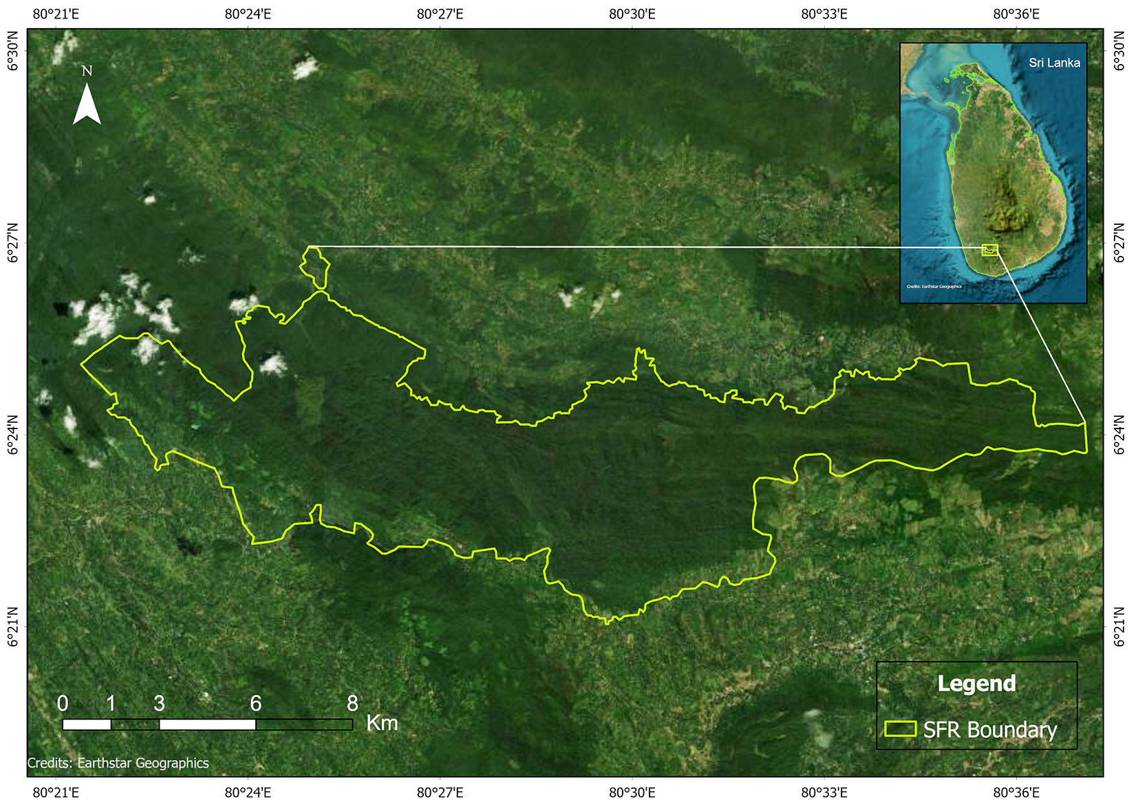
Fig. 2 - An aerial photograph of SFR that partially exhibits the vertical profile and canopy strata.
Data acquisition and vegetation categorization
Landsat 8 and Sentinel 2 data
In order to obtain spatial and spectral information on vegetation types and land cover, we obtained multi-spectral images from Landsat 8 (launched in February 2013), Sentinel 2A (launched in June 2015), and Sentinel 2B (launched in March 2017) satellites from the United States Geological Survey online database (http://glovis.usgs.gov/). Landsat 8 images were orthorectified and terrain-corrected in the T1 collection (OLI_TIRS sensor/path_141/row_56). We used bands 2, 3, 4, 5, 6, and 7 of Landsat 8, which were acquired on February 20, 2019. Two Sentinel scenes were required to cover the study area, and images from Sentinel 2A (RA076, T44NMN) and 2B (RA119, T44) were used, taken in January 2022 and November 2021, respectively. The bands considered were 2 to 11. These spectral bands were combined in ArcGIS Pro (ESRI, Redlands, USA) to create multiband raster datasets using the’ Composite Bands’ tool. Several band combinations were used to obtain rich vegetation information and discriminate between vegetation, water, and dry land ([35]). We generated raster layers of several spectral indices, as listed in Tab. 1. Additionally, GEDI-derived PAI, PAVD vegetation indices, and canopy height were included in the initial set of variables. Elevation data was obtained using a Digital Elevation Model (DEM).
Tab. 1 - Summary of spectral indices, vegetation/environmental parameters, and standard methods used (X indicates whether each parameter was considered in the final analysis).
| Parameter | Abbreviation | Method followed | Usage |
|---|---|---|---|
| Normalized Difference Vegetation Index | NDVI | NDVI is calculated from the reflectance values of two bands of electromagnetic radiation: near-infrared (NIR) and red ([19], [37]). NDVI = (NIR - RED) / (NIR + RED). | X |
| Bare Soil Index | BSI | The short-wave infrared and the red spectral bands are used to quantify the soil mineral composition, while the blue and the near-infrared spectral bands are used to enhance the presence of vegetation ([44]). (B11 + B4) - (B8 + B2) / (B11 + B4) + (B8 + B2). | X |
| Normalized Difference Moisture Index | NDMI | Normalized Difference Moisture Index is sensitive to variations in water content in leaves and can be useful for monitoring drought conditions, assessing vegetation health, and studying hydrological processes ([37]). (NIR - SWIR) / (NIR + SWIR). | - |
| Normalized Difference Water Index | NDWI | Average by quadrates (ocular estimation) | - |
| Moisture Stress Index (MSI) | MSI | The values of this index range from 0 to more than 3, with the common range for green vegetation being 0.2 to 2 ([31]). B11 / B08. | - |
| Plant Area Index | PAI | GEDI derived. | X |
| Plant Area Volume Density | PAVD | GEDI derived. | X |
| Canopy Height Model (at rh95) | CHM95 | GEDI derived. | X |
| Elevation | ele | GEDI derived + DEMs from Advanced Spaceborne Thermal Emission and Reflection Radiometer (ASTER) dataset. | X |
Topographic data
Digital Elevation Model (DEM) for the study area was obtained from version 3 of Advanced Spaceborne Thermal Emission and Reflection Radiometer (ASTER) GDEM data available at the United States Geological Survey online database (⇒ https://earthexplorer.usgs.gov/). The ASTER GDEM Version 3 data are available in GeoTIFF format at a spatial resolution of 1 arcsecond (approximately 30 meters horizontal posting at the equator). The relationship between canopy height and elevation was investigated using the DEM extracted for SFR.
Categorization of vegetation types based on PCA analysis
Raster maps were generated for elevation, NDVI, GNDVI, NDMI, BSI, NDWI, CHM95, PAI and PAVD. IDW interpolation method was utilized for the generation of raster maps based on point data from CHM95, PAI and PAVD. The values contained in these raster maps were extracted into 131 randomly generated points in ArcMap. The covariate selection process was carried out in three steps: (1) removal of covariates with variance close to zero; (2) removal by correlation; and (3) removal by importance ([8]). This ensured that statistically insignificant covariates, multicollinearity, and covariates without contextual relevance were removed before the analysis. Principal component analysis (PCA) in R version 4.3.3 ([40]) was performed to create clusters of similar vegetation/Land cover (LC) based on the standardized dataset. After accounting for multicollinearity (>75%), the number of covariates considered for the final analysis was four, which included elevation, CHM95, NDVI, BSI, and PAVD. The ground survey data and visual identification were aided to predict the vegetation/LC category of each point.
Supervised classification of satellite images to generate vegetation/LC map
We conducted supervised classification for both Landsat 8 and Sentinel 2 images. However, the Sentinel 2 classification was retained, which resulted in higher accuracy. The spectral bands 2 to 11 were combined in ArcGIS Pro (Esri, Redlands, USA) to create a multiband raster dataset using the’ Composite Bands’ tool. Training samples were provided based on both ground survey data and visual observations. The generated raster maps of vegetation indices and forest vertical structure were also used to provide training samples. The training sample data set was supplemented with Arc GIS base map imagery data (Esri, Digital Globe) when clarifications of vegetation cover were required for inaccessible terrain and locations outside the survey areas. Major vegetation types identified from PCA were considered when providing training samples; High Forest (HF), Low Forest (LF), Sub-montane Forest (SMF), Home Gardens (HG). In addition to the main four categories observed from PCA, we included four other categories that were confirmed through ground surveys, albeit with very limited area coverage. Those included Grassland/Shrubland (GS), Other Vegetation (OV) (including cropland, plantation, and degraded forest), Marsh/Swamp (MS), and Waterbody/River (WR). Therefore, a total of eight classes were considered. Due to the close resemblance between HF and LF, we describe HF as mature forests with tall trees, typically part of primary or climax forest ecosystems, characterized by a rich and complex canopy. These are often associated with older, structurally diverse forests that have achieved a stable ecological state. LF can be described as areas with shorter trees and a less developed canopy structure. These may be secondary forests, degraded forests recovering from disturbances such as logging, or forests that grow in areas with less fertile soil or more challenging climatic conditions. Thus, HF and LF will be treated as separate habitat entities henceforth. Supervised image classification was conducted based on the maximum likelihood classification (MLC) algorithm. Removal of random noise was conducted through post-classification processing, which involved majority filtering, boundary cleaning, region grouping, setting null, and nibbling.
Reference data, ground truthing, and accuracy assessment
For classifier training and validation of the satellite-image-based classification, we used ground truth data acquired during field surveys conducted between January 2019 and May 2022. The field surveys covered diverse forest types of SFR, strategically selected to encompass varying entry points to the forest and also at different altitude levels following a stratified method. The ground truth data collection involved a set of randomly generated sampling points within each major forest type, totaling 132 survey points. The forest type at each sampling point, along with the average canopy height, was recorded. A minimum of three height measurements were obtained using a Prime 1700 Laser Range Finder (Bushnell, USA) within a 20 m radius from the sampling point. The points that could not be reached or assessed via ground-based surveys were investigated using the visual inspection method. We visually inspected multitemporal imagery in Google Earth Pro and ArcGIS base maps to identify the types of vegetation and land use. The assistance of forest rangers was obtained for the validation in instances where visual inspection was inconclusive.
An accuracy assessment was conducted to compare the predicted results (classification results) with ground reference data collected from both field observations and high-resolution base map imagery. Accuracy was validated using field observations and base-map imagery. An error matrix was prepared to evaluate classification accuracy, with both overall accuracy and class-specific accuracies calculated. Additionally, we computed the Kappa coefficient (κ) in ArcGIS Pro to assess the statistical reliability of the classifications relative to random chance. The Kappa coefficient (κ) was calculated using the equation (eqn. 1):
where po represents the observed accuracy (the proportion of correctly classified samples), and pe represents the expected accuracy, which is the probability of random agreement among classifications. pe was calculated by summing the products of row and column totals for each class in the error matrix, divided by the square of the total number of samples (eqn. 2):
where ni+ and n+i are the row and column totals for class i, and N is the total number of samples. The Kappa coefficient ranges from -1 to 1, where values closer to 1 indicate stronger agreement between predicted and reference classifications.
Data acquisition and analysis of the spatial dynamics of forest structure
GEDI data
The GEDI spaceborne LiDAR system on board the International Space Station has near-global coverage between 51.6 ° and -51.6 ° latitude. The lasers on board produce four beams, resulting in eight-track ground transects. Geolocated waveforms are generated based on the laser energy return, which is tracked as a function of time. Several higher-level GEDI products are available following the processing of these waveforms. We utilized GEDI-derived Level 2A (L2A) and Level 2B (L2B) data to obtain measurements of forest canopy height, vertical canopy structure, and surface elevation. GEDI L2A data contain the coordinates, elevation, and relative height metrics (rh 0-100) extracted from return waveforms of the various reflecting surfaces located within each laser footprint. GEDI also possesses an accuracy of less than 1 m bias in canopy height measurement ([46]). The GEDI L2B standard data product adds vertical profile metrics: the canopy cover (CCGEDI), plant area index (PAI), estimated vertical canopy directional gap probability for the selected L2A algorithm (PGP_THT), foliage height diversity index (FHD), and plant area volume density (PAVD) for each laser footprint located on the land surface. A bounding box extending the area of SFR was used to select all the GEDI beams within the study area. We retrieved GEDI laser shots available from 2019 to October 2022 (Fig. S1) from NASA LP DAAC (The Land Processes Distributed Active Archive Center: https://lpdaac.usgs.gov/product_search/). The downloaded GEDI granules in HDF5 format were processed in R version 4.3.3 ([40]) using the rGEDI package ([43]) to subset and generate shape files usable in ArcGIS Pro (ESRI, Redlands, USA). We filtered only the high-quality GEDI shots for the study area using the attribute Quality Flag (QF=1) and Sensitivity (SF<0.9). We disregarded all other shots to meet the quality criteria based on energy, sensitivity, amplitude, and real-time surface tracking ([15], [14]). For canopy height metrics, we used the rh95 values of the L2A product, which is defined as the elevation difference between ground elevation and the elevation where the accumulated waveform energy is 95% of the total ([38], [46]). Using L2B granules, the PAI was obtained as cumulative values to represent the prominent forest strata at heights of 5-15 m (Lower canopy, including the understory), 15-30 m (Sub canopy), and >30m (Canopy) levels ([20]) and as an overall cumulative value from 0-45m for mapping. PAVD was also obtained for the same height categories.
Results
Vegetation categorization and mapping
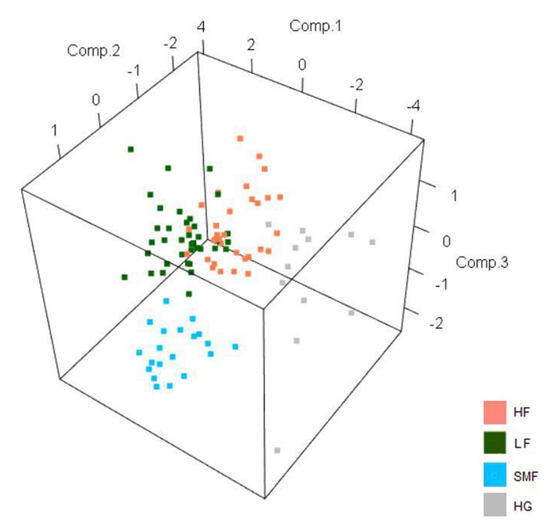
The principal component analysis revealed four major vegetation types; High Forest (HF), Low Forest (LF), Sub-montane Forest (SMF), Home Gardens (HG), and a considerable clustering was observed between the vegetation classes (Fig. 3). Based on the Eigen correlation matrix (Tab. 2), the first three principal components contributed for 84% variance. BCI and NDVI contributed significantly to PC1, which clustered the HG with other vegetation types. Significant components in PC2 were CHM and PAVD, where HF and LF were separated. Canopy height can be used as a demarcating factor for HF and LF, and we propose considering lowland areas with a 15-25 m canopy as LF and those with a canopy height of>25 m as HF. Elevation was significantly contributing to PC3 influencing the clustering of SMF (Tab. 3).
Fig. 3 - PCA 3D plot along the three principal component axes, displaying the main vegetation categories derived from the PCA analysis.
Tab. 2 - Eigen analysis of the Correlation Matrix.
| Variable | PC1 | PC2 | PC3 | PC4 | PC5 |
|---|---|---|---|---|---|
| Eigenvalue | 1.922 | 1.387 | 0.936 | 0.442 | 0.314 |
| Proportion | 0.384 | 0.277 | 0.187 | 0.088 | 0.063 |
| Cumulative | 0.384 | 0.662 | 0.849 | 0.937 | 1.000 |
Tab. 3 - Eigenvector matrix of principal components with variable scores.
| Variable | PC1 | PC2 | PC3 | PC4 | PC5 |
|---|---|---|---|---|---|
| Elevation | -0.285 | 0.209 | -0.896 | -0.269 | -0.020 |
| CHM (rh95) | 0.385 | 0.600 | 0.192 | -0.551 | -0.389 |
| BSI | 0.559 | -0.367 | -0.139 | -0.459 | 0.568 |
| NDVI | -0.532 | 0.380 | 0.329 | -0.282 | 0.621 |
| PAVD | 0.419 | 0.563 | -0.184 | 0.578 | 0.373 |
In addition to the four major vegetation/LC classes, SFR comprises four other minor vegetation/LC classes, which were identified during our ground surveys as well as in the image classification (Fig. 4). Those include Marsh/Swamp (MS), Grassland/Shrublands (GS), Other vegetation (OV) and Waterbodies (river/stream) (WR). The accuracy of the classification is indicated by the overall Kappa coefficient value of 0.9 (Tab. 4). Except for the MS category, all other classes recorded accuracy values >0.7. HF was the most dominant vegetation type, covering 38% of the area and extending over 4.355.8 ha. It was followed by LF, covering 29% of the area (Tab. 5).
Fig. 4 - Vegetation and Land cover map of Sinharaja Forest Reserve (the map may not exclusively represent the legislated boundary).
Tab. 4 - Kappa coefficient accuracy matrix for classified SFR map. Overall kappa was 0.9.
| - | Home Gardens/ | Marsh/ Swamp |
Low Dense Forest | Grassland/ Shrubland |
Dense Forest | Other vegetation | Waterbodies | Sub-montane Forest | Total | User Accuracy |
|---|---|---|---|---|---|---|---|---|---|---|
| Home Gardens/Croplands | 10.0 | 0.0 | 0.0 | 0.0 | 0.0 | 0.0 | 0.0 | 0.0 | 10.0 | 1.0 |
| Marsh/Swamp | 0.0 | 7.0 | 2.0 | 1.0 | 0.0 | 0.0 | 0.0 | 0.0 | 10.0 | 0.7 |
| Low Forest | 0.0 | 0.0 | 27.0 | 0.0 | 0.0 | 0.0 | 0.0 | 0.0 | 27.0 | 1.0 |
| Grassland/Shrubland | 0.0 | 0.0 | 2.0 | 7.0 | 0.0 | 1.0 | 0.0 | 0.0 | 10.0 | 0.7 |
| High Forest | 0.0 | 0.0 | 3.0 | 0.0 | 32.0 | 0.0 | 0.0 | 2.0 | 37.0 | 0.9 |
| Forest Plantations | 0.0 | 0.0 | 1.0 | 0.0 | 1.0 | 8.0 | 0.0 | 0.0 | 10.0 | 0.8 |
| Waterbody/River | 2.0 | 0.0 | 0.0 | 0.0 | 0.0 | 0.0 | 8.0 | 0.0 | 10.0 | 0.8 |
| Sub-montane Forest | 0.0 | 0.0 | 0.0 | 0.0 | 0.0 | 0.0 | 0.0 | 18.0 | 18.0 | 1.0 |
| Total | 12.0 | 6.0 | 35.0 | 8.0 | 34.0 | 9.0 | 8.0 | 20.0 | 132.0 | - |
| Production Accuracy | 0.8 | 1.0 | 0.8 | 0.9 | 0.9 | 0.9 | 1.0 | 0.9 | 0.0 | 0.9 |
Tab. 5 - Percentage coverage and actual area of different vegetation/land cover types.
| Vegetation/Land cover type | Percentage land cover (%) |
Area (ha) | Area (km2) |
|---|---|---|---|
| High Forest (HF) | 38 | 4355.8 | 43.6 |
| Low Forest (LF) | 29 | 3307.6 | 33.1 |
| Sub-montane Forest (SMF) | 18 | 2059.9 | 20.6 |
| Other Vegetation (OV) | 5 | 536.8 | 5.4 |
| Home Gardens (HG) | 6 | 732.4 | 7.32 |
| Grassland/Shrubland (GS) | 2 | 233.1 | 2.3 |
| Waterbody/River (WR) | 1 | 125.6 | 1.3 |
| Marsh/Swamp (MS) | 1 | 87.7 | 0.9 |
| Total | - | 11439 | 114.4 |
Vegetation and spatial dynamics
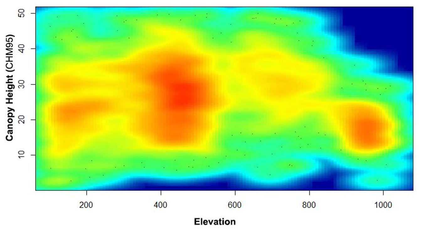
A total of 7566 GEDI footprints were present within the study area before filtering (Fig. S1). It was reduced to 1778 and 1848, respectively, for GEDI L2A and GEDI L2B, following the filtering for quality and degraded footprints. When canopy height values were plotted against elevation, the canopy height reached a peak around 500 m a.s.l. and gradually decreased at high altitudes in the Morningside region of Eastern Sinharaja (Fig. 5). A maximum NDVI of 0.86 was present within the forest vegetation, and the NDVI greatly fluctuates at different parts of the forest landscape (average: 0.44 ± 0.01) (Fig. S2b). Overall, the rich vegetation density of SFR is visible from the NDVI map. PAI of a single canopy stratum ranged between 0 to 9.79 (average: 1.96 ± 0.02), and a similar pattern was observed for PAVD, which ranged from 0 to 1.22 (0.16 ± 0.001) (Fig. S2c, Fig. S2d). When cumulative PAI values at different canopy strata were plotted against the main four vegetation classes (Fig. S3), the low overall PAI at all three canopy layers was visible for HG. The variation was limited among the other three major vegetation types. However, the higher PAI at high and mid-canopy layers of HF was visible from the violin plot, while LF and SMF had a relatively lower distribution of PAI values, respectively. As Fig. S4 depicts, the variability of PAVD at different canopy strata and the influence of total canopy height on PAVD are clearly visible (Fig. S4a, b, c, d, and e).
Fig. 5 - Variation of GEDI-derived canopy height (CHM, rh95) with elevation (Heat map range: High point density - red, Low point density - blue).
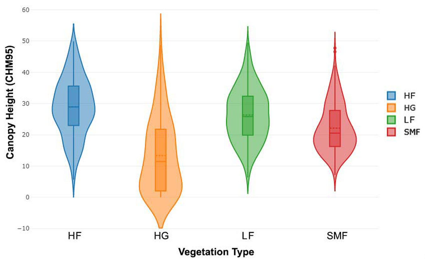
Of the main four vegetation/LC categories, the canopy height was lowest at HG (average: 13.35 ± 1.15). The second-lowest canopy height among the top four vegetation types was SMF (Average: 22.12 ± 0.42). The highest canopy heights were observed in HF (Average: 29.01±0.39) and LF (Average: 25.34±0.37) (Fig. S2e and Fig. 6), which reached maximum heights of >60 m occasionally.
Fig. 6 - Canopy height violin plot for the major vegetation types.
Discussion
Our study which focused on delineating the vegetation and land cover patterns within SFR identified eight distinct categories, highlighting the complexity of vegetation and land cover patterns in the area. However, four prominent categories HF, LF, SMF, and HGÂÂdominate the landscape, covering the majority of SFR. Both HF and LF areas fall under the tropical lowland wet evergreen rainforest ecosystem described by Gunatilleke et al. ([22]), with distinctions arising from past selective logging and naturally low vegetation density, including canopy cover. This prompted us to treat HF and LF as separate habitat entities in our analysis. We refrained from using terms like "Primary Forest" and "Secondary Forest"/"semi-logged forest" as they inadequately represented the current state of the forest, particularly given the substantial succession in semi-logged areas and variable vegetation density, especially in ridge forest areas. These two categories collectively constitute 67% of the forest reserve, representing areas of climax vegetation. HF areas primarily consist of remnants of climax tropical lowland wet evergreen rainforest, including selectively logged areas that have undergone succession. Notably, the sub-montane forest is confined to elevations ~900m asl, in line with the description of Gunatilleke et al. ([22]), covering an area of 18%, predominantly in the eastern part of the reserve known as the "Morningside". Despite being designated as a Man and Biosphere Reserve, human settlements and cultivated landscapes occupy less than 15% of the total area, with the remaining area comprising small clusters of grasslands and shrublands, marshes and swamps, and water bodies, such as rivers and streams. This habitat diversity underscores the complexity of the vegetation and land cover mosaic characteristics of this World Heritage Forest landscape.
The elevation gradient of the forest reserve is vividly portrayed in the elevation map (Fig. S2a) with the complex terrain that encompasses the region. Elevation proves to be a significant factor in shaping vegetation types in SFR. Our findings align with the work of Ediriweera et al. ([16]) regarding the negative relationship between canopy height and elevation at higher altitudes. However, we found a positive trend between canopy height and elevation up to 500m, which was not reported in previous studies (Fig. 5).
A noteworthy observation is the highest Plant Area Index (PAI) of low canopy recorded in LF areas, likely due to ongoing succession fuelled by increased sunlight penetration through upper canopy openings. Consistent with previous studies, low PAI in Sub-montane forests (SMF) at higher altitudes correlates with declines in leaf area index above 1000m, as noted by Madhumali et al. ([32]). When plotted against canopy height, Plant Area Volume Density (PAVD) illustrated distinct variations among major vegetation classes, with HF exhibiting the densest vegetation structure, followed by LF, SMF, and GS.
Elevation exerts a pronounced influence on canopy height, reflecting climatic variability. Mid-elevation areas have the highest average canopy height, while elevations above 500m experience decreased heights due to wind impacts, creating an intermediate vegetation structure between tropical lowland and montane forests, which we identify as sub-montane forests. However, ridge areas also exhibit relatively lower canopy heights, while valleys have the tallest trees, sometimes reaching >60m. The average canopy height for lowland forests is 25-30 m, dropping to ~20 m in sub-montane forests. Areas of home gardens and croplands are characterized by lower canopy heights, ranging from 0-15m. PAI and PAVD also display a similar pattern, with the highest values in valley areas and lower values in ridges and higher elevations.
This study marks the first attempt to utilize GEDI data for assessing forest canopy height and structural dynamics in Sri Lanka. Wang et al. ([46]) identified GEDI as a next-generation spaceborne LiDAR capable of revolutionizing global measurements of vertical vegetation structure. While NASA GEDI data and satellite imagery from Landsat 8 and Sentinel-2 have greatly enhanced our ability to analyze forest canopy structure and classification, several limitations and uncertainties should be acknowledged. GEDI’s data coverage is limited by its spatial sampling pattern, which is determined by the International Space Station’s orbit and the instrument’s footprint distribution. This creates gaps in GEDI coverage, particularly in regions outside the main orbital path, reducing the representativeness of the data across the entire study area. Additionally, GEDI’s vertical resolution is sensitive to terrain variations, making it less accurate in areas with steep slopes, where ground elevation and vegetation height may be misinterpreted. Both Landsat 8 and Sentinel-2 provide high-resolution multispectral imagery suitable for vegetation classification; however, their spatial resolution limits the detection of fine-scale forest heterogeneity, potentially leading to classification errors in mixed-vegetation areas or small forest patches.
SFR, being one of the most biodiverse rainforest ecosystems in the world, is of significant national and international importance. Our study fills the void regarding an updated vegetation map for the area. The versatility of GEDI database facilitated further investigation into the spatial dynamics of forest structure, particularly vertical dynamics. While acknowledging the significant contributions of long-term forest plot-based research ([1], [10], [20]), we emphasize the need for holistic spatial approaches that encompass larger areas, thereby providing a broader understanding of spatial forest dynamics. Spaceborne LiDAR, as well as aerial LiDAR, can be identified as novel remote sensing techniques with greater potential for such research endeavors. Furthermore, our findings underscore the significance of spatial and remote sensing approaches, such as spaceborne LiDAR and multispectral remote sensing, in comprehensively understanding complex tropical forest ecosystems. By highlighting the practical application of these techniques, our study advocates for their broader adoption in future research endeavors aimed at elucidating forest dynamics.
The findings of this study have important implications for the forest management and conservation of SFR. By providing a high-resolution, spatially detailed vegetation map and insights into the vertical forest structure, this research offers a comprehensive understanding of the spatial composition of SFR. The methods followed in our work provide a reliable framework for detecting deforestation, forest degradation, and habitat fragmentation over time, enabling early intervention to mitigate these threats. Moreover, identifying areas with dense vegetation presents opportunities for targeted conservation strategies. These insights support adaptive, evidence-based forest management policies that enhance climate resilience, promote long-term monitoring, and strengthen the conservation of tropical rainforest ecosystems such as Sinharaja.
Conclusion
This paper presents an updated vegetation/LC map generated for SFR with greater precision, spatial accuracy, and spatial resolution. Eight distinct land cover types were identified during this work utilizing modern remote sensing methods such as spaceborne LiDAR and multispectral satellite imagery. With the aid of NASA’s GEDI datasets, the spatial dynamics of SFR were investigated in detail for the first time, filling the current research gap. The results generated can be effectively utilized for conservation and management purposes, serving as an essential foundation for future ecological research.
Author Contributions
D.J. and D.M. conceived and conceptualized the research. DJ designed the methodology; D.J., D.M., T.D., V.M., H.S., P.G., M.G., T.P. conducted field surveys. D.J. conducted the formal analysis. D.J. wrote the first draft and D.M., V.M. reviewed and edited the manuscript. All authors discussed the results, provided feedback on the manuscript, and approved the final draft.
Conflicts of Interest
The authors declare that they have no competing interests.
Acknowledgment
The authors would like to acknowledge the support received from the staff of SFR, including Mr. Waththegama (Forester). We would also like to express our gratitude to the University of Sri Jayewardenepura for the facilities granted and the financial support provided to conduct this research under the university grant (ID: ASP/01/RE/SCI/2018/31). Funding provided by the Rufford Small Grants program (ID: 31593-1) is also acknowledged.
References
Gscholar
Gscholar
Gscholar
CrossRef | Gscholar
Gscholar
Gscholar
CrossRef | Gscholar
CrossRef | Gscholar
Gscholar
CrossRef | Gscholar
Authors’ Info
Authors’ Affiliation
Tharanga Dhananjani 0000-0001-8446-4678
Dharshani Mahaulpatha 0000-0002-6563-7462
Department of Zoology, Faculty of Applied Sciences, University of Sri Jayewardenepura, Gangodawila (Sri Lanka)
Vinuri Mendis 0009-0006-3540-0006
Faculty of Graduate Studies, University of Sri Jayewardenepura, Gangodawila (Sri Lanka)
Faculty of Graduate Studies, University of Manitoba, Winnipeg, Manitoba, R3T 2N2 (Canada)
Faculty of Applied Sciences, Uva Wellassa University, Badulla 90000 (Sri Lanka)
Faculty of Technology, University of Sri Jayewardenepura (Sri Lanka)
Corresponding author
Paper Info
Citation
Jayasekara D, Dhananjani T, Mendis V, Jayawickrama H, Prasad T, Gunarathna MM, Gunarathna P, Mahaulpatha D (2025). Mapping the vegetation and spatial dynamics of Sinharaja tropical rain forest incorporating NASA’s GEDI spaceborne LiDAR data and multispectral satellite images. iForest 18: 45-53. - doi: 10.3832/ifor4632-017
Academic Editor
Marco Borghetti
Paper history
Received: Apr 26, 2024
Accepted: Dec 05, 2024
First online: Apr 01, 2025
Publication Date: Apr 30, 2025
Publication Time: 3.90 months
Copyright Information
© SISEF - The Italian Society of Silviculture and Forest Ecology 2025
Open Access
This article is distributed under the terms of the Creative Commons Attribution-Non Commercial 4.0 International (https://creativecommons.org/licenses/by-nc/4.0/), which permits unrestricted use, distribution, and reproduction in any medium, provided you give appropriate credit to the original author(s) and the source, provide a link to the Creative Commons license, and indicate if changes were made.

Web Metrics
Breakdown by View Type
Article Usage
Total Article Views: 13435
(from publication date up to now)
Breakdown by View Type
HTML Page Views: 7458
Abstract Page Views: 2752
PDF Downloads: 2903
Citation/Reference Downloads: 0
XML Downloads: 322
Web Metrics
Days since publication: 460
Overall contacts: 13435
Avg. contacts per week: 204.45
Article Citations
Article citations are based on data periodically collected from the Clarivate Web of Science web site
(last update: Mar 2025)
(No citations were found up to date. Please come back later)
Publication Metrics
by Dimensions ©
Articles citing this article
List of the papers citing this article based on CrossRef Cited-by.
Related Contents
iForest Similar Articles
Review Papers
Remote sensing-supported vegetation parameters for regional climate models: a brief review
vol. 3, pp. 98-101 (online: 15 July 2010)
Review Papers
Accuracy of determining specific parameters of the urban forest using remote sensing
vol. 12, pp. 498-510 (online: 02 December 2019)
Review Papers
Remote sensing of selective logging in tropical forests: current state and future directions
vol. 13, pp. 286-300 (online: 10 July 2020)
Research Articles
Afforestation monitoring through automatic analysis of 36-years Landsat Best Available Composites
vol. 15, pp. 220-228 (online: 12 July 2022)
Technical Reports
Detecting tree water deficit by very low altitude remote sensing
vol. 10, pp. 215-219 (online: 11 February 2017)
Review Papers
Remote sensing support for post fire forest management
vol. 1, pp. 6-12 (online: 28 February 2008)
Research Articles
Assessing the performance of MODIS and VIIRS active fire products in the monitoring of wildfires: a case study in Turkey
vol. 15, pp. 85-94 (online: 19 March 2022)
Technical Reports
Remote sensing of american maple in alluvial forests: a case study in an island complex of the Loire valley (France)
vol. 13, pp. 409-416 (online: 16 September 2020)
Research Articles
Geostatistical techniques for estimating aboveground biomass in eastern Amazonia
vol. 19, pp. 85-93 (online: 13 March 2026)
Research Articles
Assessing water quality by remote sensing in small lakes: the case study of Monticchio lakes in southern Italy
vol. 2, pp. 154-161 (online: 30 July 2009)
iForest Database Search
Search By Author
Search By Keyword
Google Scholar Search
Citing Articles
Search By Author
Search By Keywords
PubMed Search
Search By Author
Search By Keyword


