Use of δ13C as water stress indicator and potential silvicultural decision support tool in Pinus radiata stand management in South Africa
iForest - Biogeosciences and Forestry, Volume 12, Issue 1, Pages 51-60 (2019)
doi: https://doi.org/10.3832/ifor2628-011
Published: Jan 24, 2019 - Copyright © 2019 SISEF
Research Articles
Abstract
In this study, the carbon isotope ratio in tree rings was investigated as a potential measure of water availability and drought stress in Pinus radiata stands in South Africa. An understanding of water availability and its variation in space is fundamental to the implementation of increasingly site-specific management regimes that have the potential to improve stand productivity. Fourteen plantation compartments, situated on water shedding (convex) terrain were identified where reliable weather data existed and a water balance model could be run. This output was used to derive water stress indicators: (a) relative canopy conductance (gc/gcmax) and (b) the ratio of actual to potential evapotranspiration (ETa/ETp). The water stress indicators (calculated per year of growth) were related to δ13C values in five tree rings formed in the five years before mid-rotation thinning took place. The water balance model used adequately described soil water availability throughout each growing season and indicated that most severe stand water stress occurred during the summer months of the study period (November to April). The ETa/ETp ratio for this period as well as the relative canopy conductance proved to be good measures of water stress. The 5-year averages of the ETa/ETp ratios (taken over the driest 6 month period) ranged from 0.17 to 0.32 (winter rainfall zone) and 0.44 to 0.70 (all-year rainfall zone). The 5-year averages of ETa/ETp ratios could be accurately predicted (p< 0.0001; adjusted r2 = 0.83) with multiple regression using δ13C values in whole-wood samples (i.e., earlywood and latewood) and the site index of stands (where site index is the average height of the dominant 20% trees in the stand at base age 20). The δ13C values in tree rings across the planted range of P. radiata in South Africa can therefore be used to identify broad categories of water availability for purposes of increasingly site-specific silvicultural management.
Keywords
Stable Carbon Isotope, Tree Rings, Water Availability, Drought Stress, Site-specific Forest Management, Monterey Pine
Introduction
The availability of adequate soil water for tree growth is fundamental to forest productivity in South Africa. Water distribution and its reliability is a significant problem, and is therefore a major consideration when decisions on plantation establishment and site-species matching are made ([11], [12]). Water stressed stands are less likely to respond to increased availability of other growth resources (light and nutrients) as water stress inhibits cell expansion, carbon assimilation and changes carbon partitioning patterns to favour root growth ([7]). For example, water stressed stands will seldom show significant growth responses following fertilisation ([22]) and fertilising such stands would constitute an unnecessary financial expense. But just how can the degree of water stress a stand is experiencing over seasons and years be quantified for use in management decisions (i.e., on a forest compartment or landscape scale)? This question can potentially be answered by a number of promising approaches:
(1) Constructing a daily water balance using detailed climatic and soil information ([3], [33], [31]). This is only feasible where a very dense network of detailed weather data on the landscape and detailed soil information is available, which is often not the case in Southern African forests. If a soil is enriched with water from upslope positions the construction of the water balance moves to a high degree of complexity with unacceptably high sources of potential error (see Tab. S1 in supplementary material);
(2) Establishing a relationship between stand water stress and remotely sensed indices of evapotranspiration on a limited number of experimental sites and extrapolating this across the landscape ([2]). This technique relies on an array of satellite images of a particular forest estate that are well spaced in time intervals which is not always available;
(3) Establishing a relationship between stand water use and the ratio of carbon isotopes sequestered by the stand during photosynthesis and extrapolating this across the landscape ([37]). One major advantage of this technique is that the isotope ratio is preserved in the tree rings and that it can be sampled retrospectively.
This study focused on the application of carbon isotope fractionation, a technique that has been studied intensively in forestry applications since the 1980’s. It has been shown that a relationship exists between the extent of carbon isotope discrimination and plant water use efficiency ([38]) as well as water availability ([23], [37], [20]). Atmospheric carbon dioxide (CO2) consists of approximately 98.9% carbon-12 (12C) and 1.1% carbon-13 (13C) ([28]). Both of these are stable isotopes of carbon. When a plant absorbs CO2 from the atmosphere during photosynthesis, it discriminates among isotopes due to small differences in their chemical and physical properties (described in more detail below). Isotopic ratio mass spectrometry (IRMS) is used to determine the 13C content of samples converted to CO2 by combustion in order to determine the ratio R, defined as (eqn. 1):
R values are converted to values of δ13C for convenience ([28] - eqn. 2):
where the original standard was CO2 obtained from Pee Dee Belemnite (PDB).
One of the most widely used models to explain changes in the isotopic sequences of tree rings were described by Francey & Farquhar ([16]). There are two stages during which discrimination against 13C takes place: during the diffusion of atmospheric CO2 through the stomata, where the isotopic content of the CO2 is altered by fractionation, and at the biochemical level where the enzyme Ribulose-1.5-biphosphate carboxylase discriminates against 13C due to its lower reactivity ([28]).
Farquhar et al. ([13]) determined that the extent of discrimination that takes place during the uptake of CO2 from the atmosphere is determined by the ratio of intercellular to ambient CO2 concentrations (ci/ca). This is the balance between the inward diffusion of CO2 which is controlled by stomatal conductance (gc) and the CO2 assimilation (which depends on the rate of photosynthesis - [36]). If stomatal diffusion is rapid (gc is high), and the carboxylation process of photosynthesis is limiting, the predicted δ13C value will be more negative than when stomatal diffusion is slow (gc is low - [28]). Therefore, a combination of factors, e.g., water availability and plant nutrition (which affect both the rates of photosynthesis and gc), may be reflected in the δ13C ratio of plant tissues.
At the stand level, various authors ([23], [36], [37], [20]) have reported that δ13C is strongly influenced by the availability of soil water. During periods where water availability is low, the δ13C values are less negative which implies that the discrimination against 13C is lower. This is due to the fact that gc is low because transpiration is minimised through the closing or partial closing of stomatal guard cells. Warren and co-workers ([37]) also found large variations in δ13C as a result of thinning and fertilisation. They concluded that δ13C is only a useful indicator of soil water availability or drought stress in seasonally dry climates if the variation in other environmental factors (such as nutritional status and radiation interception) can be accounted for. In stands with similar age, stocking and nutritional status, it is thus possible that isotope fractionation could be related to the degree of water stress a stand is experiencing over specific periods during its lifetime. With information on soil water availability, more informed decisions about silvicultural practices, such as fertilisation, thinning, and site-species matching may be made.
The primary objective of this study was to develop a management tool for foresters. We investigated whether the degree of water stress experienced by mid-rotation stands of Pinus radiata could be estimated using δ13C values from wood samples. A secondary objective was to test if ancillary variables related to site factors, tree competition or soil fertility could be used as covariates to improve such estimates of water stress. To minimise unwanted variation, managed plantation forests of P. radiata in their mid-rotation were chosen as study objects because they have comparable stand density and age (two factors that are known to affect the δ13C values in wood). It is during mid-rotation that several decisions must be made regarding thinning intensity and fertilisation in plantation forests, choices that need to be viable for several years following implementation. Given that water stress may vary considerably from year to year, a specific focus was placed on the relationship between the average water stress over a number of years prior to mid-rotation thinning and the average δ13C values in wood that was formed during the corresponding period.
Material and methods
The focus of this study was to regress δ13C values in wood samples from a range of sites with varying water stress on a well-recognised indicator of plant water stress, namely the ratio of actual to potential evapotranspiration (Eta/Etp, described below). The use of covariates relating to site factors, competing vegetation and soil fertility were also investigated. We therefore describe the collection of three main data sets in the Materials and Methods section as follows: (a) the site-related information (some of which were tested as covariates); (b) the determination of water stress indicators (which is determined using a water balance model with, inter alia, climatic data and soil water holding capacity as inputs); and (c) the determination of the δ13C values in wood samples.
(a) Site selection and description
From the literature, four categories of factors are known to affect the δ13C values in wood samples: plant water stress, competing vegetation, soil fertility and other site factors (related to plant physiological response). Plant water stress was the main focus of our study, and therefore we aimed to minimise variation where possible in the other three categories during site selection. In addition, we chose variables related to each of the remaining three categories for potential use as covariates in the regression analysis, and each of these are briefly mentioned here and discussed more comprehensively below. Factors related to competing vegetation included stand age, quadratic mean diameter (Dq), stand density, stand basal area, age of first thinning and stand density index (SDI). Site factors included mean annual temperature (MAT), altitude and site index (SI). Finally, the single factor related to soil fertility was clay content.
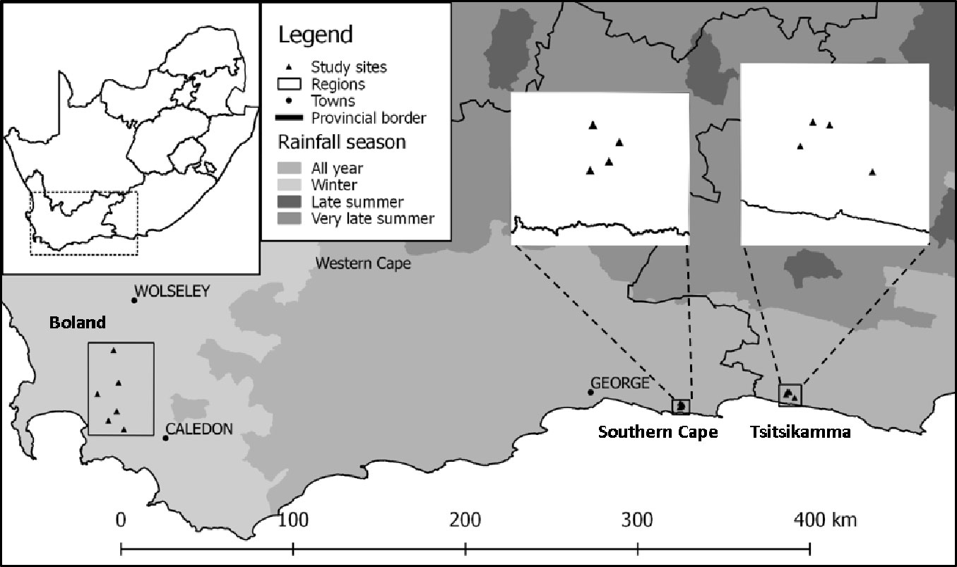
In order to minimise random variation, stands with similar age and stocking were selected. Using management information supplied by Mountain to Ocean Forestry (MTO), plantation compartments of an age between 12 and 16 years, managed on a regular silvicultural regime were selected as this coincides with the time when silvicultural choices need to be made using information on water stress that the stand is likely to experience. For inclusion in the shortlist, these compartments additionally needed to be scheduled for a mid-rotation thinning during the year of sampling or would have had a first thinning the previous year as thinning could have an influence on δ13C values ([37]). After preliminary screening, field inspections were carried out to determine the suitability of each stand for inclusion into the study. Care was taken to select only compartments on high points in the landscape (convex terrain units) in order to minimise the effect of subsurface water flow or water logging conditions on δ13C values. Fourteen trial sites were selected to include sites from the winter rainfall area (Boland) as well as from the all-year rainfall areas (Southern Cape and Tsitsikamma), to ensure coverage of a wide range of water availabilities. A typical mid rotation Pinus radiata stand in the Tsitsikamma is shown in Fig. S1 (Supplementary material) for illustrative purposes.
In order to simulate water availability with the aid of an accurate, daily water balance, chosen compartments had to be located within two kilometres of a reliable weather station. Stand characteristics of the chosen trial sites, as well as summarised meteorological information, are given in Tab. 1 and trial site locations are depicted graphically in Fig. 1. There is a general increase in the quantity of rainfall and the duration of the rainy season from west to east for the sample sites depicted in Fig. 1. Note that sites using the same weather station were chosen such that soil profiles (and hence water storage characteristics) were markedly different.
Tab. 1 - Characteristics of trial sites used to investigate the potential of δ13C as a drought stress indicator. (Dq): Quadratic mean diameter at breast height (cm); (SI): site index at age 20 (m); (BA): basal area (m2 ha-1); (PTPH): planted trees per hectare; (CTPH): current trees per hectare; (Soil profile water): maximum available soil water in mm if the profile is at field capacity.
| Comp’t. no. | Plantation | Latitude | Longitude | Altitude (m a.s.l.) |
Age (yr) | Dq (cm) | BA (m2 ha-1) |
SI (m) | PTPH | CTPH | Age of first thinning (yr) |
Mean annual rainfall (mm) |
Soil profile water (mm) |
Mean Air Temp (°C) |
|---|---|---|---|---|---|---|---|---|---|---|---|---|---|---|
| L35b | Haweqwas | -33.710 | 19.052 | 408 | 12 | 17 | 20 | 23.0 | 1111 | 989 | 9 | 772 | 178 | 18.4 |
| M4 | Jonkershoek | -33.971 | 18.935 | 246 | 14 | 20 | 22 | 25.0 | 816 | 727 | 13 | 1073 | 118 | 17.0 |
| G36 | Grabouw | -34.074 | 19.074 | 394 | 18 | 30 | 29 | 25.0 | 1372 | 413 | 10 | 954 | 115 | 17.1 |
| E18 | Grabouw | -34.129 | 19.015 | 350 | 14 | 19 | 23 | 23.0 | 816 | 727 | 13 | 1188 | 75 | 15.1 |
| N15a | Grabouw | -34.181 | 19.125 | 368 | 11 | 13 | 12 | 23.0 | 1087 | 967 | 13 | 773 | 178 | 16.9 |
| A35c | La Motte | -33.904 | 19.087 | 241 | 17 | 25 | 25 | 25.0 | 816 | 543 | 14 | 880 | 177 | 18.3 |
| D3d | Bluelilliesbush | -33.974 | 23.869 | 228 | 15 | 25 | 36 | 29.3 | 1372 | 473 | 8 | 1060 | 99 | 18.1 |
| D10 | Bluelilliesbush | -33.959 | 23.894 | 343 | 10 | 19 | 27 | 29.1 | 1372 | 648 | 8 | 1060 | 52 | 18.1 |
| B5a | Bluelilliesbush | -33.992 | 23.930 | 231 | 11 | 26 | 34 | 29.1 | 1372 | 645 | 7 | 1060 | 59 | 18.1 |
| D60 | Bluelilliesbush | -33.957 | 23.880 | 332 | 9 | 14 | 16 | 28.0 | 1372 | 1219 | 9 | 1060 | 105 | 18.1 |
| E2a | Kruisfontein | -34.024 | 23.111 | 270 | 16 | 22 | 28 | 26.3 | 1372 | 530 | 14 | 791 | 195 | 16.9 |
| F14c | Kruisfontein | -34.034 | 23.129 | 247 | 13 | 22 | 33 | 24.2 | 1111 | 540 | 12 | 791 | 313 | 16.9 |
| G19d | Kruisfontein | -34.050 | 23.109 | 156 | 13 | 22 | 27 | 27.2 | 1372 | 567 | 10 | 791 | 312 | 16.9 |
| G4c | Kruisfontein | -34.045 | 23.122 | 205 | 9.8 | 20 | 26 | 32.7 | 1111 | 650 | 8 | 791 | 56 | 16.9 |
Fig. 1 - Sample points for soil water stress and δ13C determination on the southern seaboard of South Africa.
In each of the plantation compartments, a plot of 25 × 25 trees was marked out in an area with uniform growth, and the diameter at breast height (DBH) for each tree was recorded. The length and width of each plot was determined in order to calculate basal area (BA) for each sample plot. The starting points of each of these length measurements were between tree rows on each side of the plot. The age of each stand at the time of sampling and the age at first thinning was obtained from plantation management records. The stand density was calculated as the number of trees per sample plot, scaled-up to a hectare. The quadratic mean diameter of trees was determined as the square root of the value (sum of squares of the DBH measurements divided by the number of trees). The stand density index was calculated for as follows (eqn. 3):
where N is the observed number of trees per hectare and Dq is the quadratic mean diameter; after Reineke (1933), as cited in Pretzsch ([30]).
The site index of pine stands in South Africa are usually expressed as the mean height of the 20% trees of largest diameter per sample plot at a reference age of 20 years. We determined the mean height of the 20% largest trees per sample plot and extrapolated this value from the current age to the reference age of 20 years using standard site index curves for South African P. radiata stands.
(b) Determination of water stress indicators
Soil sampling
Soil pits measuring approximately 1.5 × 0.5 m were dug in the centre of the plot. The depth of the pits averaged 90 cm. Topsoil samples (0-10 cm) were taken at four random points on the plot. All organic matter and forest floor litter were carefully removed to expose the mineral soil and a cylindrical sampler with a volume of 200 cm2 was hammered into the soil and then carefully removed with a shovel. All material inside the sampler was collected and the four samples were combined to represent the topsoil layer.
Inside the soil pit, the different soil horizons were visually identified and the depth of each horizon recorded. Samples were taken of each horizon from the four sides of the pit from 10 cm below the soil surface down to the bottom of the pit. To accurately describe soil water availability and to determine how deep the soil profile would be if it was opened up completely, a soil auger was used to drill down further than the bottom of the pit. Materials retrieved with the auger was also collected and bulked per horizon with depth.
Soil samples were sent to a commercial laboratory for textural analysis as well as coarse fragment percentage determination. Soil texture was determined by disaggregating the samples using sodium-hexametaphosphate and ultrasound dispersion; the coarse fragments and the three sand fractions were determined by sieving and the silt and clay fractions were determined by sedimentation using an ASTM E100 (152H-TP) hydrometer at 20 °C. The details of the methodology is described by the Non-affiliated Soil Analysis Work Committee ([27]).
Results from the textural analysis and coarse fragment determination were used to calculate the field capacity (FC) and wilting point (WP) of each soil profile, using the computer program “SOILPAR”, developed by Acutis & Donatelli ([1]). FC and WP are required input parameters for the soil water balance model used in this study. Care was taken to assign particles to the correct individual size classes since the names of size fractions in the model were not completely congruent to that of the South African texture classification system used in local laboratories. To ensure that calculations of plant-available soil water in each profile (using SOILPAR software) were realistic, the calculated values were compared to a range of soil water content values that had been published for South African forest soils with different texture classes ([34]).
Soil water balance modelling
In order to model soil water availability, the hydrological model referred to as HyMo (developed by [31]) was used. The decision to use this model was based on the fairly simple input requirements needed to run the model. Basic meteorological inputs include daily maximum and minimum temperatures, relative humidity, wind speed, precipitation and solar radiation. Where meteorological datasets were incomplete, the few missing values were replaced with long-term averages for the particular parameters. Additional site information required by the model includes latitude, longitude, altitude, as well as soil depth and soil texture, plant genus, stand age class and soil drainage class.
The model uses the Penman-Monteith equation ([3]) and a single layer soil storage value based on field capacity and wilting point. It estimates actual evapotranspiration, interception and runoff, and calculates the daily change in soil water availability as (eqn. 4):
with Δφ: change in soil water content (in mm d-1); rr: precipitation (mm d-1); eta: actual evapotranspiration (mm d-1); int: rainfall interception by canopy (mm d-1); ro: total runoff (mm d-1) cr: capillary rise (mm d-1); irr: irrigation (mm d-1).
Details on how each of the parameters is calculated by the model can be obtained in the original literature ([31]). The model has been used on stands of beech (Fagus sylvatica), spruce (Picea abies) and Scots pine (Pinus sylvestris) by the author of the model. The model has also been validated by various other studies and it can therefore be assumed that HyMo is a reliable soil water balance model with relatively simple data requirements ([8], [32], [9]).
Stand stress
In order to determine whether a stand experiences stress due to the limited availability of water, the relative extractable water (REW) was calculated according to Granier et al. ([19] - eqn. 5)
where W is the soil water content in the root zone, Wm is the lower limit of water availability, and WFC is the soil water content at field capacity.
The use of REW is beneficial to the study since it provides a single, integrated value of water availability and is strongly related to predawn water potential ([5]). Water stress is assumed to occur when REW drops below 0.4, i.e., below 40% of the maximum extractable water ([18]). Poyatos et al. ([29]) described a strong limitation of transpiration in Pinus sylvestris when REW dropped below 0.4, and for that reason the value was maintained here. This gave a clear indication of when stands started to experience stress due to inadequate water availability. Using results obtained from HyMo, monthly REW values were calculated for each trial site.
Water stress indicators
Granier & Bréda ([17]) developed a model to describe canopy conductance using environmental drivers (climate and soil water availability). Using daily values of REW they calibrated a logarithmic curve that describes the relationship between canopy conductance (gc) as a fraction of the maximum canopy conductance (gcmax) and REW (eqn. 6):
This relationship holds for pine species as well, as described in Granier et al. ([19]). Using the output generated by HyMo and expressing it as REW, the relative canopy conductance (gc/gcmax) was estimated on a daily basis (after [17]).
The water supply / demand ratio (hereafter ETa/ETp) is the ratio of actual (ETa) to potential (ETp) evapotranspiration and it reflects the magnitude of stress and the duration of conditions that are favourable for plant growth ([35]). Small ETa/ETp values indicate that the stand can only supply a small portion of the atmosphere’s evaporative demand. This is mainly due to low soil water content or large vapour pressure deficits (VPD’s). As part of its output, the HyMo model calculates the daily actual and potential evapotranspiration. The Eta/ETp ratio for various stress periods was calculated accordingly and used as a measure of stand water stress.
Calculation periods and statistical analyses
In order to ensure that the best models were selected during the analysis of the data, six periods were initially tested in a pilot study for the calculation of the average gc/gcmax and ETa/ETp. The first test period started in the middle of the six-month stress period as indicated by REW, taking the summer months of January and February into account. From there, a month was added on each side and the results were analysed again. This continued until a period of 12 months was reached. Fig. S2 in Supplementary material is a graphic representation of the periods that were initially tested in this pilot study. Using REW as a measure of moisture stress, it was possible to determine that the most severe moisture stress period experienced by trees among the study areas is the period from early summer to autumn (November to April). The water stress within this 6-month period (as indicated by either gc/gcmax or ETa/ETp) was henceforth used as the standard measurement period against which δ13C isotope ratios (see below) were correlated in this study. The correlation between water stress indicators and δ13C isotope ratios was performed for individual years and for 5-year average values (i.e., the individual water stress indicator values spanning the November to April period of 5 consecutive years were averaged, and correlated to the average carbon isotope ratio obtained from 5 corresponding year rings). This was done because rainfall can fluctuate strongly from year to year across all sites. The rationale for the 5-year averaging is that silvicultural decision support is based on characterising sites by the mean water stress that its trees are likely to experience at mid-rotation on each particular site.
(c) Timber sample processing and analysis
On each of the study sites, four co-dominant trees were randomly selected, felled and a disk with a thickness of approximately 25 mm was cut from each tree at breast height. In preparation for laboratory analysis, the disks were oven dried at 105 0C (until it reached constant mass) and was then cut in half using a small band saw. The halves were inspected and the one with the least reaction wood was selected for further analysis.
The half-disks were cut into eight segments of equal size. These segments were lightly sanded on both sides to improve the visibility of the annual growth rings. To minimise the variability of δ13C within each tree ring, four segments were randomly selected for further processing ([26], [21]). There were 14 sites with 4 sample trees per site of which two different types of samples were analysed for 13C: (i) the latewood (cellulosic fraction) of the last five growth rings; and (ii) a bulked, whole-wood sample of last five growth rings. The rationale for using the cellulosic latewood samples is that latewood growth rings are formed during periods when a tree experiences water stress, and because there will be minimal contamination from mobile organic substances. Analysing the δ13C values from latewood would thus lead to results that are focused on the period during which a tree experiences the most water stress. Bulked, whole-wood samples were also tested to assess whether a greatly simplified (and thus cheaper) sample preparation procedure would yield similar results. Starting from the youngest latewood growth ring on each segment, the late- and earlywood was split off using a hammer and sharp chisel. Five latewood growth rings representing five years before the first thinning of the plantation compartment took place were selected and all visible earlywood that was still present was removed by slicing it off with a scalpel. The sanded surfaces were also sliced off to avoid contamination from the sandpaper. Using the chisel, all the pieces of wood were then reduced to a size small enough for milling. The two sample batches (i.e., bulked, whole-wood samples and latewood samples) were then milled with a Wiley Mill® (Arthur H Thomas Co., PA, USA) and all pieces, which passed through a 40-mesh sieve, were collected. Milled samples were stored in clean glass bottles with screw cap lids and placed in desiccators.
The bulked whole-wood sample batch was not subjected to any additional pre-processing and was analysed as is for δ13C (see below), because the aim of this sample batch was to test a simplified sample preparation procedure. The latewood sample batch was subjected to an extraction of the cellulosic material, to avoid possible contamination from non-cellulosic mobile substances, (e.g., compounds like oils and resins). The extraction was performed using the acid-catalysed solvolytic method ([24]), and is briefly described here. After oven drying at 105 0C overnight, milled samples (0.5 g) were weighed (± 0.002 mg) and placed in clean 28 ml McCartney bottles; 2.65 ml of diglyme (Diethylene glycol dimethyl ether) and 0.665 ml 10M HCl were added and the bottles were sealed with screw caps with teflon-butyl liners. The bottles were then placed in a shaking water bath (SHWBD36, Scientific Manufacturing, Table View, Cape Town, South Africa) at 90 0C for three hours. After three hours the caps were removed and the residue was collected by gravity filtration. Filter paper (150 mm diameter, grade: 391) was weighed, folded into cones and placed in glass funnels in 250 ml Erlenmeyer flasks; 20 ml of methanol was used to rinse the bottles and wash the residue onto the filter paper. The residue was further washed three times with boiling water and oven-dried overnight. The mass of the dried samples was determined after it had cooled down to room temperature (approximately 23 °C) in a desiccator. Taking care not to contaminate the sample with cellulose from the filter paper, residues left on the filter paper were collected and placed in 2 ml Eppendorf tubes for further analysis.
Determination of δ13C
The δ13C value of each growth ring from the latewood sample batch, and the bulked, whole-wood sample of 5 year rings were determined at IsoEnvironmental cc, situated at the Botany Department of Rhodes University in Grahamstown, South Africa, on a Europa Scientific Elemental analyser and 20-20 IRMS. Each batch of samples analysed contained 29 internal standard samples of a reference sample that is made up of beet sugar and ammonium sulphate. Also included were five standards of Casein, a certified protein standard which had been calibrated against IAEA-CH-6 and IAEA-N-1. The overall C precision obtained from this analysis was 0.14‰.
Statistical analyses
All statistical calculations were done with the STATISTICA® software package (Statsoft Inc., USA, ver. 9). To analyse the results, two types of linear regressions were done. The first was a set of normal linear regressions with (i) gc/gcmax and (ii) ETa/ETp ratio, each time on δ13C as the independent variable. The second set of regressions tested the inclusion of one covariate from each of the categories mentioned in Section (a) of the Materials and Methods. The categories and their tested variables included: (i) stand age, Dq, stand density, stand basal area, age of first thinning and SDI in the category “competing vegetation”; (ii) MAT, altitude and SI in the category “site factors”; and (iii) clay contents in the category “soil fertility”. We only allowed the use of the variable with highest leverage in each category, because the use of highly related variables (i.e., variables within the same category) as covariates in any single regression would violate the basic rules of regression. During analysis, in the interest of parsimony, we used (i) the best three variables, and (ii) the best two variables to explain the observed range in ETa/ETp ratio.
Results
Soil water availability
From the output generated by HyMo the soil water content and REW were plotted over four years of observations to better understand the change in soil water content over time. Unique seasonal patterns were observed due to investigations of several sites within each rainfall region. These patterns remained similar among different sites within a region despite the fairly wide ranges in soil water storage capacity. Fig. 2, Fig. 3 and Fig. 4 depict the typical soil water content patterns for sites from different rainfall regions.
Fig. 2 - Modelled soil water content (a) compared to daily precipitation (b) for Comp’t. L35b (Boland region, 2003-2006).
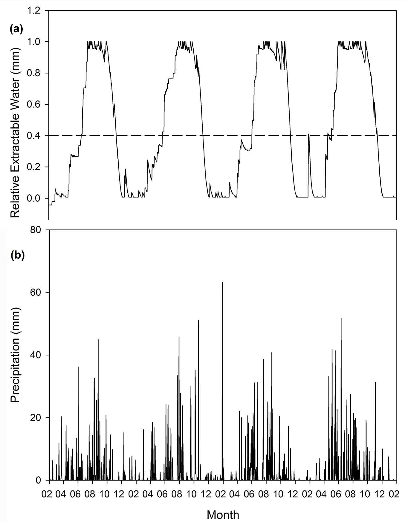
Fig. 3 - Modelled soil water content (a) compared to daily precipitation (b) for Comp’t. E2a (S-Cape region, 2003-2006).
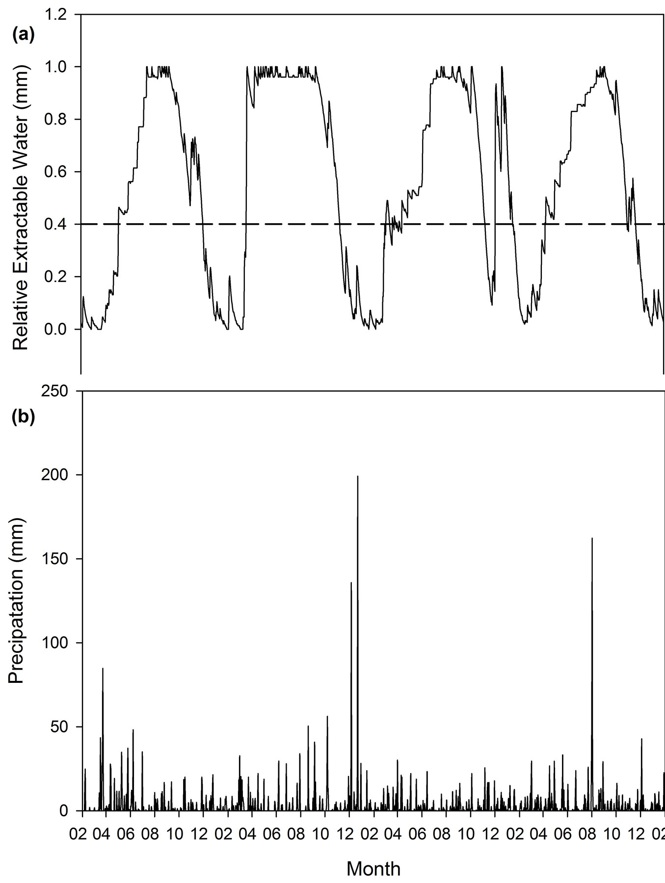
Fig. 4 - Modelled soil water content (a) compared to daily precipitation (b) for Comp’t. B5b (Tsitsikamma region, 2003-2006).
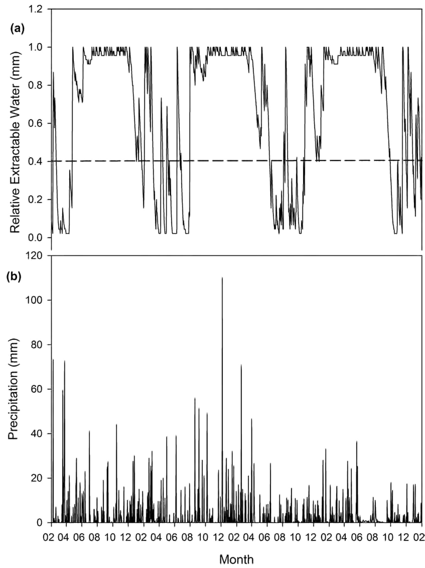
The Boland region has a pronounced seasonal effect on the soil water content with long periods where the soil water content is at the lower limit of water availability (Fig. 2). Sites in the Southern Cape area (Fig. 3) show some seasonal effects; however it is not as clear as in the Boland. The Tsitsikamma sites are located in a high rainfall area of the all-year rainfall zone of South Africa and there are fewer periods where the soil water content is at the lower limit of water availability (Fig. 4).
δ13C and stress indicators
The calculated relative canopy conductance (gc/gcmax) and supply/demand ratios (ETa/ETp) were plotted against δ13C of the individual latewood samples to investigate the relationship between the variables. On an individual sample basis, no statistically significant trends in the data were apparent (data not shown).
In order to estimate the average water stress that a stand may experience at mid rotation, the mean of five yearly values for δ13C, gc/gcmax and ETa/ETp (hereafter 5-yr means) were used for further analysis. The 5-yr means of the δ13C values and calculated water stress indicators for the corresponding period are presented in Tab. 2. The graphic investigation of the data is shown in Fig. S3 and Fig. S4 (Supplementary material). In both cases, site G19d in Southern Cape was an outlier. For a few years this site yielded δ13C values in the region of -29‰ while the other three sites had δ13C values ranging from -25‰ to -28‰. The landscape position and soil profile suggested that it may receive seepage water in the deeper subsoil despite efforts to sample only stands on water shedding sites and it was decided to exclude this site from the study. Site G19d is thus not included in Fig. 5, Fig. 6, Fig. S3, Fig. S4 (Supplementary material) nor in the multiple regressions described below.
Tab. 2 - Water availability indicators and δ13C values in wood samples for each of the trial sites. The following water availability indicators were calculated by averaging data over 5 years prior to mid-rotation thinning: mean soil water content, relative extractable water (REW), relative canopy conductance (gc/gcmax), supply / demand ratio (ETa/ETp), as well as δ13C values measured in latewood and whole-wood samples. (n.d.): not detected.
| Comp’t. | Plantation | Region | Wilting Point (mm) |
Field capacity (mm) |
δ13C [latewood] (‰) |
δ13C [whole-wood] (‰) |
Mean soil water content (mm) |
REW | gc/gcmax | ETa/ETp |
|---|---|---|---|---|---|---|---|---|---|---|
| L35b | Haweqwas | Boland | 39 | 178 | -25.34 | -26.19 | 42 | 0.12 | 0.25 | 0.23 |
| N15a | Grabouw | Boland | 25 | 118 | -24.48 | -25.80 | 37 | 0.13 | 0.22 | 0.19 |
| G36 | Grabouw | Boland | 37 | 115 | -24.78 | -26.12 | 46 | 0.13 | 0.77 | 0.21 |
| M4 | Jonkershoek | Boland | 12 | 75 | -24.68 | n.d. | 25 | 0.13 | 0.50 | 0.21 |
| A35c | LaMotte | Boland | 39 | 178 | -23.96 | -25.40 | 56 | 0.12 | 0.20 | 0.23 |
| E18 | Grabouw | Boland | 62 | 177 | -26.31 | -27.08 | 85 | 0.20 | 0.33 | 0.31 |
| E2a | Kruisfontein | S-Cape | 42 | 195 | -27.12 | -27.72 | 83 | 0.42 | 0.52 | 0.49 |
| F14c | Kruisfontein | S-Cape | 61 | 313 | -26.53 | -27.08 | 131 | 0.28 | 0.48 | 0.47 |
| G4c | Kruisfontein | S-Cape | 72 | 312 | -26.66 | -27.26 | 145 | 0.31 | 0.58 | 0.57 |
| G19d | Kruisfontein | S-Cape | 19 | 105 | -29.00 | -27.41 | 39 | 0.23 | 0.44 | 0.36 |
| B5a | Bluelilliesbush | Tsitsikamma | 11 | 56 | -27.49 | -27.01 | 24 | 0.28 | 0.52 | 0.39 |
| D3d | Bluelilliesbush | Tsitsikamma | 18 | 99 | -27.14 | -27.44 | 52 | 0.39 | 0.69 | 0.61 |
| D10 | Bluelilliesbush | Tsitsikamma | 10 | 52 | -27.60 | -27.77 | 27 | 0.40 | 0.64 | 0.55 |
| D60 | Bluelilliesbush | Tsitsikamma | 11 | 59 | -28.22 | -27.63 | 29 | 0.38 | 0.35 | 0.53 |
Fig. 5 - Relationship between 5-yr means of ETa/ETp ratio and the δ13C in whole-wood samples of corresponding tree rings. Dashed lines indicate the 95% confidence interval.
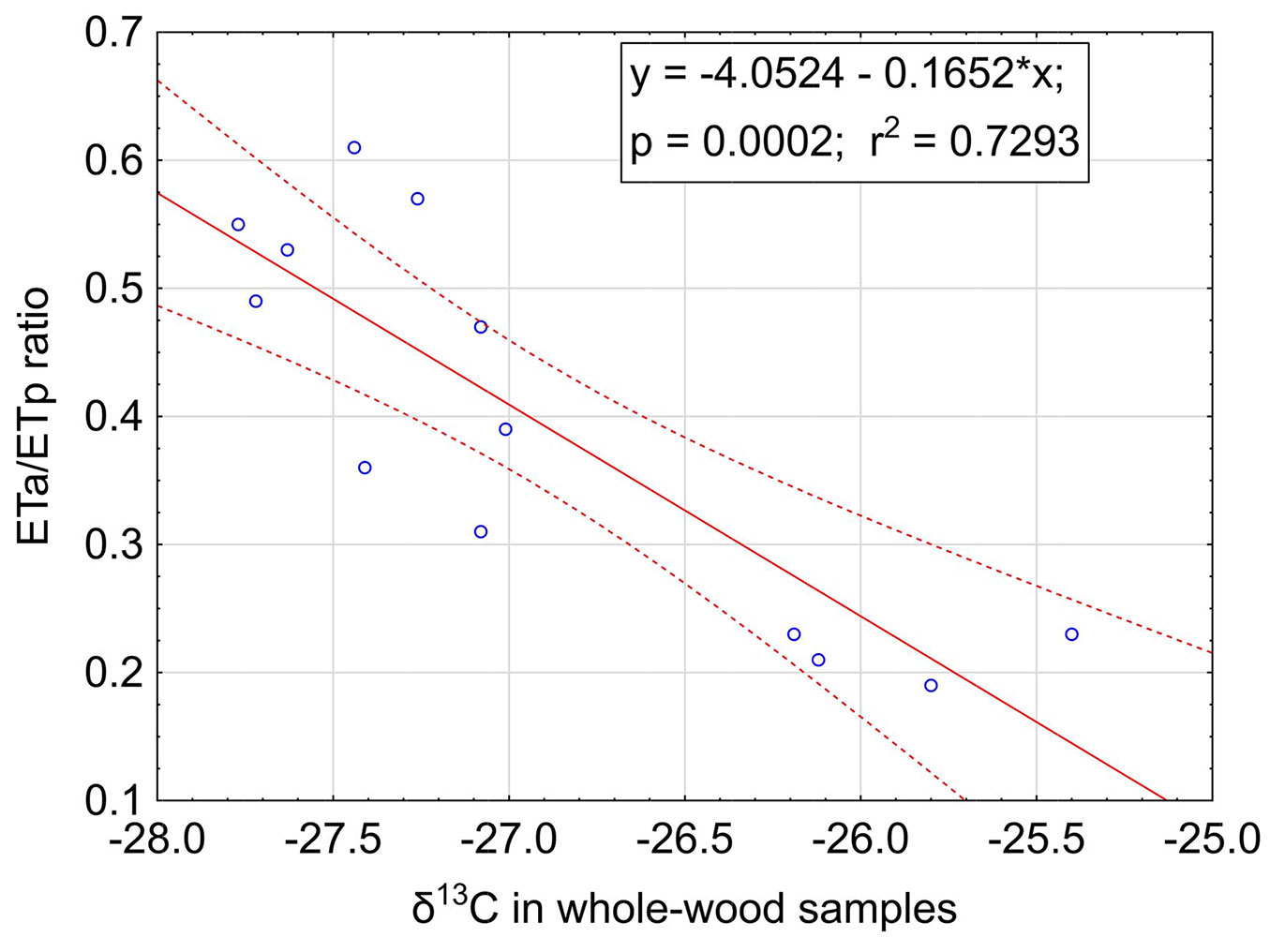
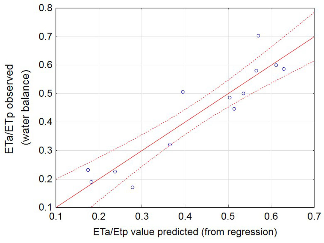
Fig. 6 - Relationship between observed and predicted ETa/ETp ratios using eqn. 7 (adj-r2 = 0.83).
With site G19d excluded, linear regressions were done with 5-year means of δ13C as an independent variable and 5-yr means of gc/gcmax and ETa/ETp, in turn, as response variables. These regressions were done for various stress periods throughout the year. For relative canopy conductance the best two models were obtained when using the average values for four and six months during the stress period. Using the ETa/ETp ratio, all the models, except for the two months in the middle of the stress period, produced a very good fit of the data. Standardising on the models to be used, the six months stress period (November to April) was chosen. Although the four-month stress period models have a similar fit, the six-month period would cover the whole stress period during a growing year.
The ANOVA results for the two models chosen to describe stand water stress using δ13C are shown in Tab. S2 (Supplementary material). Fig. S3 and Fig. S4 show the fitted regression lines with the 95% confidence intervals for both response variables. Both models fit the data very well, yielding r2 = 0.73 (p = 0.002) for gc/gcmax and r2 = 0.78 (p < 0.001) for ETa/ETp. The whole-wood sample preparation method (which does not require separation of latewood nor any extractions) was then implemented to test if the laboratory procedure could be streamlined. The relationship between the 5-year means of the ETa/ETp ratio of stands and the δ13C values of whole-wood samples is shown in Fig. 5. This relationship explains only 73% of the variability, compared to 78% when using latewood samples, but the wood sample preparation procedure for the whole wood samples is much simpler and less time consuming.
Multiple regression analyses showed the variables δ13C(latewood), SI, clay content and basal area to be the four best predictors of growth within each category of variables explained before, with the former two being significant and clay content and basal area being not significant (Tab. 3). We therefore performed a second set of multiple regressions, this time restricting the number of variables to two. The output of this analysis is shown in Tab. S3 (Supplementary material). The predictors, δ13C and site index, were both significant, and collectively explained 78% of the variation. A final multiple regression was done to predict the ratio of actual to potential evapotranspiration with the best two variables, but this time using the values obtained for δ13C in the whole wood samples. The result is shown in Tab. 4. The predictors, δ13C and site index, were both significant, and collectively explained 86% of the variation. The goodness of fit of the Eta/ ETp values (calculated with the water balance model) versus the same value (predicted with δ13C and site index values using eqn. 7) is shown in Fig. 6.
Tab. 3 - Regression summary for three best variables predicting the ratio of actual to potential evapotranspiration (ETa/ETp). R² = 0.8996; Adjusted R² = 0.849; F[4, 8] = 17.923; p<0.00047; std. error of estimate: 0.06922.
| Variable | b* | Std error of b* | b | Std error of b | t(10) | p-value |
|---|---|---|---|---|---|---|
| Intercept | - | - | -1.7296 | 0.4186 | -4.1315 | 0.0026* |
| δ13C (latewood) | -0.4547 | 0.1607 | -0.0533 | 0.0189 | -2.8291 | 0.0198* |
| Basal area | 0.0983 | 0.1461 | 0.0026 | 0.0039 | 0.6731 | 0.5178 |
| Clay contents | -0.2358 | 0.1360 | -0.0048 | 0.0028 | -1.7346 | 0.1168 |
| Site index | 0.4425 | 0.1652 | 0.0270 | 0.0101 | 2.6787 | 0.0253* |
Tab. 4 - Regression summary for two best variables predicting the ratio of actual to potential evapotranspiration (ETa/ETp) using whole wood samples to determine δ13C. R² = 0.86; Adjusted R² = 0.826; F[2, 10] = 29.541; p<0.00006; std. error of estimate: 0.07434.
| Variable | b* | Std error of b* | b | Std error of b | t(10) | p-value |
|---|---|---|---|---|---|---|
| Intercept | - | - | -4.0429 | 0.7966 | -5.0754 | 0.0005 |
| δ13C (whole wood) | -0.6195 | 0.1472 | -0.1418 | 0.0337 | -4.2086 | 0.0018 |
| Site index | 0.4169 | 0.1472 | 0.0247 | 0.0087 | 2.8321 | 0.0178 |
The following equation is thus proposed to predict ETa/ETp in P. radiata stands (eqn. 7):
where ETa/ETp(6 M) is the ratio of actual to potential evapotranspiration over 6 summer months, δ13CWW is the δ13C value in whole wood sample of 5 year rings prior to mid-rotation thinning, and SI20 is the Site index (m) at base age of 20 years.
Discussion
Soil water availability
The soil water content over time, as modelled by HyMo yields a more comprehensive understanding of the available soil water in forest stands over seasons and years in the Southern and Western Cape forestry areas. The Boland region, typified in Fig. 2, which receives winter rain, is subject to a strong seasonal pattern of soil water availability. During the winter, the soil profile stays fully charged because precipitation events are frequent and evapotranspiration is very low (the average evapotranspiration rate for June/July in the modelled sites was less than 0.1 mm d-1). With the change from winter to spring, the available soil water content declines rapidly due to increases in ETa to a point where the soil water approaches the wilting point during the hot, dry summer. The rapid depletion of available soil water stems from the fact that plant-available water in modelled Boland soil profiles ranges from 75 to 178 mm and the corresponding daily evapotranspiration rates for October-November average around 3 mm day-1. This rapid depletion of soil water is also reflected in the gc/gcmax and ETa/ETp values for the Boland sites.
The sites in the Southern Cape (typified in Fig. 3) show a more gradual change in soil water content over time. The periods where the soil water content is almost at the wilting point are shorter and these are frequently interrupted by precipitation. The result is that gc/gcmax and ETa/ETp for these areas are higher, indicating less moisture stress. During June and July, the VPD in the region is generally so low that evapotranspiration drops to very low levels. In the Boland the ETp rises sharply from October to January. The ETa however decreases rapidly from November to January as the soil profile dries out, the VPD rises and stand stress sets in. In the Southern Cape and Tsitsikamma areas (typified in Fig. 3 and Fig. 4), the increase in ETp from October to January is not as severe as in the Boland with the onset of summer. The intervals between rainfall events are also shorter which provides forests stands with larger amounts of available water. This leads to smaller decrease in ETa than in Boland. The amount of solar radiation that the regions receive also differs. The Southern Cape and Tsitsikamma areas regularly receive mist that reduces solar radiation, while the Boland area has more cloud free days, especially in summer.
The locations of sample sites were chosen so that they were positioned on water shedding locations. The effect of this selection process was that the sample sites represent the drier end of the spectrum on the plantation estates. The average 12-month ETa/ETp values for the study sites ranged from 0.30 in the Boland to 0.56 in the Southern Cape and 0.73 in the Tsitsikamma area. When comparing these results with relative extractable water typically held in the soil profiles, it becomes clear that the shorter interval between rainfall events in the Southern Cape and Tsitsikamma area, especially during the summer months, makes more water available in the soil profile with a reduction in stand stress, leading to increased stand productivity. We standardised our analyses on the Eta/ETp values over the 6 summer months, which means that the ETa/ETp values are lower than the annual values, especially in the Boland region which has a Mediterranean climate pattern and where the lowest values occur. In contrast to the 12-month values, the 6-month Eta/ETp values range from 0.17 to 0.63 (Fig. 5).
δ13C and stress indicators
On an individual year and growth ring basis, the weak correlation between δ13C and either gc/gcmax or ETa/ETp indicates that there still is a lot of unexplained variation (data not shown). We acknowledge that some portion of the variation in δ13C among individual years could be due to sampling error, failure to detect false tree rings, measurement error or a possible “carry over” effect that could be present between growing seasons. However, there is a pronounced change in intraspecific tree competition in plantations during the period from 5 years before mid-rotation thinning (trees usually relatively free growing) up to the months before actual thinning (trees under strong competition). Such changes in tree competition are known to affect the δ13C signature in wood samples. Furthermore, where trees increase in size, asymmetric competition will lead to a disproportionate amount of resource use by the larger trees and smaller trees will experience water stress as they are deprived of water. The aim of this research is not to characterise individual tree response to water stress, but rather the average water stress that the stand is experiencing, as this will influence silvicultural decisions. As a management tool, it will thus be more informative to work with the averaged δ13C signature in the last 5 year rings prior to mid rotation thinning (obtained from four co-dominant trees, as stated in the methodology). In this way, the values obtained will not be specific to a given year or individual tree or a degree of intraspecific competition in the stand, but rather reflect an average degree of water stress that the stand may have experienced over this period.
The patterns that emerged from testing the influence of several variables per category during multiple regression are discussed below. In addition to δ13C, the most influential variables per category were clay contents, basal area and SI, of which only SI was significant.
An increase in the clay content of a soil will increase the water holding capacity per unit soil depth. The clay contents of sites L35b, G36, N15a, G19d and G4c fell in the range of 19-24%, which is moderately high compared to all the remaining sites that had clay contents below 8% ([15]). However, water availability to trees in any given site cannot be gauged by clay contents alone. It is governed by the interplay between rainfall distribution and soil water storage capacity (the latter being dependent mainly on soil texture and soil depth). Seeing that clay content is only one of the key contributing factors to soil water availability, it explains the rather weak and non-significant influence (p = 0.1168) that clay contents exhibits on ETa/ETp values (Tab. 3).
The basal area of a stand is influenced by the stand density and the diameter of the trees in any particular stand. Basal area is moderately well correlated to leaf area index (and hence to the transpirational surface) of the canopy of a given stand. Working on Pinus radiata in New Zealand, Warren et al. ([37]) reported that δ13C values were more negative in stands with 750 stems ha-1 than in stands with 250 stems ha-1, indicating greater water stress. We tried to narrow down the range in stocking and mean diameter in our experimental plots so as to develop regressions that will be realistic for managed stands of P. radiata. The stands used in this research project only ranged from 413 to 1219 stems per hectare, which may contribute to the fact that the effect of basal area on the regressions was noticeable but not significant (Tab. 3).
When calculating site index, the mean height of the 20% largest diameter trees at age 20 is used. Site index is thus a measure of site quality and growth resource availability. Better soil fertility, adequate rainfall and favourable terrain position will contribute towards a less stressed stand and improved tree growth. As a result, the site index has a significant influence on the prediction of ETa/ETp ratios (p = 0.0253 - Tab. S3 in Supplementary material). Site index values per compartment do not have to be specially measured as these data sets are readily available in virtually all plantation management systems. Using SI as a covariate does therefore not place an additional burden of data collection on the prediction process. The δ13C values had the strongest influence on predicting ETa/ETp ratios, both as latewood (p = 0.0122) and whole wood samples (p = 0.0018 - Tab. S3 and Tab. 4). Both latewood and whole wood samples were useful in determining Eta/ ETp ratios, suggesting that intensive sample preparation (i.e., separating late- and earlywood, followed by extraction of cellulosic compounds from the latewood) does not necessarily add value to the prediction of ETa/ETp. Using whole wood samples would simplify the sampling process and bring down the cost of analysis substantially.
As stated before, foresters could benefit from gauging the average water stress plantation stands experience at mid-rotation age as it is likely to have an impact on stand responsiveness to silvicultural treatments. Following the protocol set out here, co-dominant trees, which are removed during the first thinning operation, can be sampled as they are removed from the stand anyway, eliminating the need to sample among the remaining trees. A further improvement on the sampling technique would be to take timber cores at breast height instead of whole disks. Several commercial timber companies routinely collect tree cores to gauge wood properties and δ13C could easily be determined from such samples.
By integrating the δ13C values obtained during each thinning into a geographic information system, representative values for stand stress across a whole plantation can be mapped and used for future site/ species matching and silvicultural decisions. For example, fertilisation seldom yields satisfactory responses under conditions of stand water stress. Decisions on whether to fertilise a particular stand would thus be made easier if the likelihood of water stress on a given site can be predicted, based on the SI and average δ13C value in the wood. Values indicating lower stress conditions would mean that more soil water is available for use by the stand and thus the likelihood and magnitude of response to fertilisation would be greater ([22], [10], [6]). Stands experiencing water stress (as indicated by low gc/gcmax or ETa/ETp values) will shift their carbon allocation patterns and more carbon will be allocated to root growth ([4]). Under such conditions fertilisation may not have the desired effect of improving stem volume growth and may result in a financial loss to the forest grower. A second example is that of thinning: thinning operations often affect the soil water availability and may also affect the water use efficiency of stands ([25], [14]). It is possible that an indicator of average soil water stress before thinning (such as δ13C) on a given site could be a useful tool in deciding which thinning intensity should be implemented.
We concede that the addition of more sites to the dataset from which the current proposed model has been developed may increase the predictive power of the model. However, we argue that the δ13C values in whole wood samples and their associated site indices can already be used as presented in Fig. 6 to predict broad categories of water availability classes using eqn. 7, and that this result has potential to assist with silvicultural decision making.
Conclusions
δ13C values differ not only between rainfall regions, but also within the same region. Lower soil water availability results in less negative δ13C values and is strongly related to the different measures of stand water stress investigated in this study. The use of δ13C and site index as predictors of the soil water stress that plantation stands experience is a tool that could potentially be used in decision support systems regarding silvicultural and drought risk management.
Acknowledgements
The authors express their sincere thanks to the THRIP programme of the National Research Foundation, in partnership with Wild Peach Investment Holdings and MTO Forestry for financial support. We also thank Dr. Thomas Rötzer and the FORSIM project for assistance with the water balance model; Mr. Anton Kunneke for GIS support; Proff. Thomas Seifert and Tim Rypstra for advice, Mr. Daan Nel for support with statistical analyses and our technical helpers (Mr. Henry Solomon and Mr. Philip Truter) who assisted with sample preparation. We acknowledge the South African Weather Services as well as the Agriculture Research Council for the use of their meteorological data.
References
Gscholar
Gscholar
Gscholar
Gscholar
CrossRef | Gscholar
Gscholar
Gscholar
Gscholar
Authors’ Info
Authors’ Affiliation
Ben du Toit
Department of Forest and Wood Science, University of Stellenbosch, Private Bag X1, Matieland, Stellenbosch, 7602 (South Africa)
Sappi Forests (Pty) Ltd, P.O. Box 372, Ngodwana, 1209 (South Africa)
Corresponding author
Paper Info
Citation
Fischer PM, du Toit B (2019). Use of δ13C as water stress indicator and potential silvicultural decision support tool in Pinus radiata stand management in South Africa. iForest 12: 51-60. - doi: 10.3832/ifor2628-011
Academic Editor
Tamir Klein
Paper history
Received: Sep 08, 2017
Accepted: Nov 15, 2018
First online: Jan 24, 2019
Publication Date: Feb 28, 2019
Publication Time: 2.33 months
Copyright Information
© SISEF - The Italian Society of Silviculture and Forest Ecology 2019
Open Access
This article is distributed under the terms of the Creative Commons Attribution-Non Commercial 4.0 International (https://creativecommons.org/licenses/by-nc/4.0/), which permits unrestricted use, distribution, and reproduction in any medium, provided you give appropriate credit to the original author(s) and the source, provide a link to the Creative Commons license, and indicate if changes were made.

Web Metrics
Breakdown by View Type
Article Usage
Total Article Views: 48287
(from publication date up to now)
Breakdown by View Type
HTML Page Views: 38530
Abstract Page Views: 4683
PDF Downloads: 4193
Citation/Reference Downloads: 1
XML Downloads: 880
Web Metrics
Days since publication: 2710
Overall contacts: 48287
Avg. contacts per week: 124.73
Article Citations
Article citations are based on data periodically collected from the Clarivate Web of Science web site
(last update: Mar 2025)
Total number of cites (since 2019): 8
Average cites per year: 1.14
Publication Metrics
by Dimensions ©
Articles citing this article
List of the papers citing this article based on CrossRef Cited-by.
Related Contents
iForest Similar Articles
Research Articles
Testing a dual isotope model to track carbon and water gas exchanges in a Mediterranean forest
vol. 2, pp. 59-66 (online: 18 March 2009)
Research Articles
Soil water deficit as a tool to measure water stress and inform silvicultural management in the Cape Forest Regions, South Africa
vol. 13, pp. 473-481 (online: 01 November 2020)
Short Communications
Preliminary indications for diverging heat and drought sensitivities in Norway spruce and Scots pine in Central Europe
vol. 13, pp. 89-91 (online: 01 March 2020)
Review Papers
Drought-induced mortality of Scots pines at the southern limits of its distribution in Europe: causes and consequences
vol. 3, pp. 95-97 (online: 15 July 2010)
Research Articles
Effect of drought stress on some growth, morphological, physiological, and biochemical parameters of two different populations of Quercus brantii
vol. 11, pp. 212-220 (online: 01 March 2018)
Research Articles
Spatial and temporal variation of drought impact on black locust (Robinia pseudoacacia L.) water status and growth
vol. 8, pp. 743-747 (online: 18 June 2015)
Research Articles
Oak sprouts grow better than seedlings under drought stress
vol. 9, pp. 529-535 (online: 17 March 2016)
Research Articles
Recovery of water potential and leaf gas exchange performance following drought stress in Quercus cerris populations
vol. 19, pp. 94-101 (online: 17 March 2026)
Research Articles
Gas exchange, biomass allocation and water-use efficiency in response to elevated CO2 and drought in andiroba (Carapa surinamensis, Meliaceae)
vol. 12, pp. 61-68 (online: 24 January 2019)
Research Articles
Addressing post-transplant summer water stress in Pinus pinea and Quercus ilex seedlings
vol. 8, pp. 348-358 (online: 16 September 2014)
iForest Database Search
Search By Author
Search By Keyword
Google Scholar Search
Citing Articles
Search By Author
Search By Keywords
PubMed Search
Search By Author
Search By Keyword


