Are the new gridded DSM/DTMs of the Piemonte Region (Italy) proper for forestry? A fast and simple approach for a posteriori metric assessment
iForest - Biogeosciences and Forestry, Volume 9, Issue 6, Pages 901-909 (2016)
doi: https://doi.org/10.3832/ifor1992-009
Published: Aug 29, 2016 - Copyright © 2016 SISEF
Research Articles
Abstract
Aerial LiDAR (Light Detection and Ranging) derived data are widely adopted for the study and characterization of forests. In particular, LiDAR derived-CHM (Canopy Height Model) has proved essential in identifying tree height variability and estimating many forest features such as biomass and wood volume. However, CHM quality may be affected by internal limits and anomalies caused by raw data (point cloud) processing (i.e., vertical errors), which are quite often disregarded by users, thus generating potentially erroneous results in their applications. In this work, an auto-consistent procedure for the fast evaluation of CHM accuracy has been developed based on the assessment of internal anomalies affecting CHM data obtained by differencing gridded DSM (Digital Surface Model) and DTM (Digital Terrain Model). To this purpose, a CHM was generated using the gridded DTMs and DSMs provided by the Cartographic Office of the Piemonte Region (north-western Italy). We estimated the local potential CHM error over the whole region, and demonstrated its strictly dependence on the terrain morphometry, particularly slope. The relationship between potential CHM error and slope was modeled separately for mountain, hill and flat terrain contexts, and used to produce a potential error map over the whole region. Our results showed that approximately 20% of the regional territory suffers from CHM uncertainty (in particular high elevation areas, including the treeline), though the majority of regional forest categories was affected by negligible CHM error. The potential consequences of CHM error in forest applications were evaluated, concluding that the tested LiDAR dataset provide a reliable basis for forest applications in most of the regional territory.
Keywords
ALS, LiDAR, CHM, Data Quality, Vertical Errors, Slope Effect, Forest Applications
Introduction
Aerial LiDAR (Light Detection and Ranging) is nowadays one of the most used remote sensing technologies for studying and characterizing forests. Due to its excellent accuracy, LiDAR-derived datasets can provide reliable estimations of many forest structural characteristics, such as tree height, canopy height variability and closure ([7]). Moreover, tree vertical distribution can be directly retrieved, while above-ground biomass, average basal area, average stem diameter, canopy volume and tree density can be modeled ([6]).
LiDAR raw data are point clouds that can be directly interpreted. Nevertheless, it is quite common to operate using gridded LiDAR data obtained from point clouds (raw data) by spatial regularization or interpolation. A Digital Surface Model (DSM) and the correspondent Digital Terrain Model (DTM) can be jointly used to retrieve by differencing the so called Canopy Height Model (CHM). In the case of forests, CHM is a measure of the trees’ height over the considered area and can be used to assess many fundamental forest parameters such as biomass and wood volume, and is proving to be increasingly useful to identify canopy height variability and detect tree crowns ([13], [18]).
ALS (Aerial Laser Scanning) data have been also proposed to map treeline height position and shifts ([16]). Treelines are transition ecotones very sensitive to temperature regimes and considered as ecological indicators of climate change. With rising temperatures, treeline is expected to colonize tree-less areas located at higher altitudes. Therefore, it is important to monitor the position and the possible movements of these ecotones, and LiDAR derived data may represent a useful tool to this purpose. However, regardless the mapping strategy adopted, results often are affected by uncertainty that should be clearly assessed and notified.
Despite the importance of LiDAR datasets in forest applications, the internal limits and anomalies caused by raw data quality and pre-processing are quite often disregarded or neglected. Indeed, such constraints can impact the effectiveness and reliability of measures in specific applications, generating potentially erroneous results. Nowadays, LiDAR derived datasets are often freely available from institutional and non-institutional subjects, and provided to customers “ready to use”. Ideally, quantitative estimates of data quality measures (pulse return coordinate accuracy and precision, conformity with required specifications, data spatial consistency and completeness) should be part of every laser data delivery. However, such information is often incomplete or even missing, due to the costly and time-consuming procedures for data quality evaluation ([8]), especially in mountain areas. Moreover, quality measures supplied to end-users within metadata frequently refer to the original data (i.e., point cloud) and not to the derived gridded dataset, which is generally characterized by a higher uncertainty due to the regularization/interpolation process.
For these reasons, users may greatly benefit from the possibility of testing the quality of data to be used, especially when mountain forest contexts are regarded. Few scientific papers dealing with LiDAR-derived data have considered this aspect ([9]). Conversely, some scientific works use LiDAR datasets as reference for validating measurements obtained by other remote sensing systems ([10], [25]). In general, this procedure is deemed feasible as vertical and horizontal accuracy of LiDAR measures is much higher (average vertical accuracy: 0.15 m - [2]) compared to most remotely sensed data (e.g., Landsat, MODIS, etc.). Nonetheless, LiDAR raw data often require a pre-processing step to avoid uncontrolled artifacts (i.e., vertical errors), especially after point cloud gridding/interpolation ([1]).
CHM uncertainty strictly depends on the reliability of the gridded DTM/DSM from which it derives by differencing. It is well known that vertical error is related to topography ([12]), land cover categories ([9]), vegetation classes ([5]) and canopy density ([22]). In particular, the joint effect of LiDAR acquisition geometry and terrain slope can emphasize these errors ([14]). Since steep slopes can increase vertical absolute errors ([24]), height measurements of trees located in these areas potentially suffer from higher uncertainty. Nevertheless, only few works have taken into consideration the effect of topography on DTM/DSM/CHM accuracy ([23]).
The aim of this work was to develop a new approach for estimating CHM vertical uncertainty without any ground survey information. CHM was obtained here by matrix difference from DSM and DTM freely available in a grid format from the Cartographic Office of the Piemonte Region (NW Italy). These represent the most common data provided by public institutions to end-users and researchers not directly involved in LiDAR point clouds processing. We developed a fast method to quantify and map CHM uncertainty over the study area, regardless the method used to attain the grid from the original LiDAR data. We also explored the dependence of CHM uncertainty from topography and pointed out its effects in forest applications.
Materials and methods
Approach description
The proposed approach is based on a dataset validation method to identify “evident artifacts” affecting the CHM obtained by subtracting DSM from DTM grid values. Grids showing negative differences are obviously CHM errors (artifacts), as DSM values should locally be equal or higher than those of the DTM. No direct field validation survey was possible nor required, as our goal was explicitly to develop a ready-to-use and auto-consistent procedure for a fast evaluation of CHM uncertainty. Our objectives were: (i) to quantify the uncertainty of the tested dataset; (ii) to propose a fast and simple CHM validation methodology; (ii) to show the potential limitation due to CHM uncertainty in respect to forestry applications in the Piemonte Region.
For this tasks, 96 sample DSM and DTM tiles representing three different landscape contexts (flat, hilly and mountainous areas) were selected. For each tile, the correspondent CHM was obtained and several synthetic statistics computed. CHM errors due to artifacts were then analyzed and related to their landscape characteristics to test for possible effects of terrain morphometric parameters. The main focus was on slope that is considered the most conditioning factor, according to the literature ([24]). Terrain effects on CHM uncertainty were then modeled, and CHM errors were mapped over the whole Piemonte Region. Moreover, we investigated if and how the estimated CHM uncertainty affects the main regional forest categories. Particular attention was paid to forest categories located at the highest elevation where the treeline occurs. In most interpretations, the treeline represents either the upper altitudinal or latitudinal line connecting trees having a minimum height of 2-5 m ([11]). In this context, the vertical accuracy in tree height measurement obtained from the CHM becomes crucial for early detection of pioneer trees representing the ongoing tree migration ([17]).
All computations and statistics were run and managed by SAGA® GIS (System for Automated Scientific Analysis, Hamburg, Germany) and IDL (Interactive Data Language) programming tools.
Dataset
The LiDAR dataset of the Piemonte Region has been recently released in a gridded format (DTM and DSM) covering the entire regional territory. The dataset was acquired during the ICE aerial-photogrammetric survey (2009-2011). Relative flight height was about 4500 m a.s.l, with a longitudinal and cross overlapping of 55-70% and 90%, respectively ([20]). LiDAR point clouds were acquired using a LEICA ALS50-II sensor ([15]). Nominal point density was about 0.5 points m-2. The system was capable of detecting up to 4 multiple returns for each outbound laser pulse (first, second, third, last). The vertical discrimination distance between consequent pulses was approximately 3.5 m. DTM and DSM were pre-processed from the original LiDAR point clouds by filtering and regularization, resulting in a geometric resolution of 5 m.
The reference technical report concerning DTM quality check ([19]) states that “data control is considered positive if no more than 5% of ΔQ differences results (in absolute value) higher than 0.60 m; moreover, for areas defined as of «reduced accuracy», i.e., mountainous forest areas, threshold value is set to 1.44 m”. Since these reference values are as much as twice the DSM/DTM precision (tolerance), we assumed the tolerance as a statistical measure of CHM uncertainty (errors). The regional cartographic department states that the DSM dataset is “not explicitly tested” because it represents an intermediate product in the generation of the DTM. Since no specification were given, we assumed the same tolerance for DSM and DTM. All data were delivered in the UTM 32N WGS84 reference frame. DTM tile size matches the correspondent 1:10.000 section of the Regional Technical Map (CTR).
A land cover map of “Forests and other territory covers” (FTC) was also obtained in a vector format from the regional database (SIFOR - [21]). The FTC reference frame is the UTM WGS-84 zone 32N, with nominal scale 1:10.000. The FTC includes 5 major classes of territory cover: “agricultural areas”, “predominant pastoral value areas”, “semi-natural herbaceous formations”, “forested areas”, “other territory covers”. The “forested areas” class includes 93 forest types and 21 forest categories.
Study area
Piemonte extends for about 2.539.983 ha, of which 1.098.677 ha are covered by mountains, 769.848 ha by hills and 671.458 ha by lowlands. Forest areas cover about 916.000 ha ([4]). In order to allow a representative selection of the entire regional framework, sample areas used in this study were extracted from each landscape context, which was thus represented by a different number of DTM/ DSM tiles distributed over the whole region (Fig. 1). Sample tiles were selected according to the administrative boundaries of municipalities whose territory is mostly mountainous, hilly or flat. Overall, 96 tiles were selected for the following municipalities:
Fig. 1 - Geographic distribution of the selected sample DTM/DSM tiles over the Piemonte Region. (Dark green): lowland tiles; (pale green): hill tiles; (brown): mountain tiles.
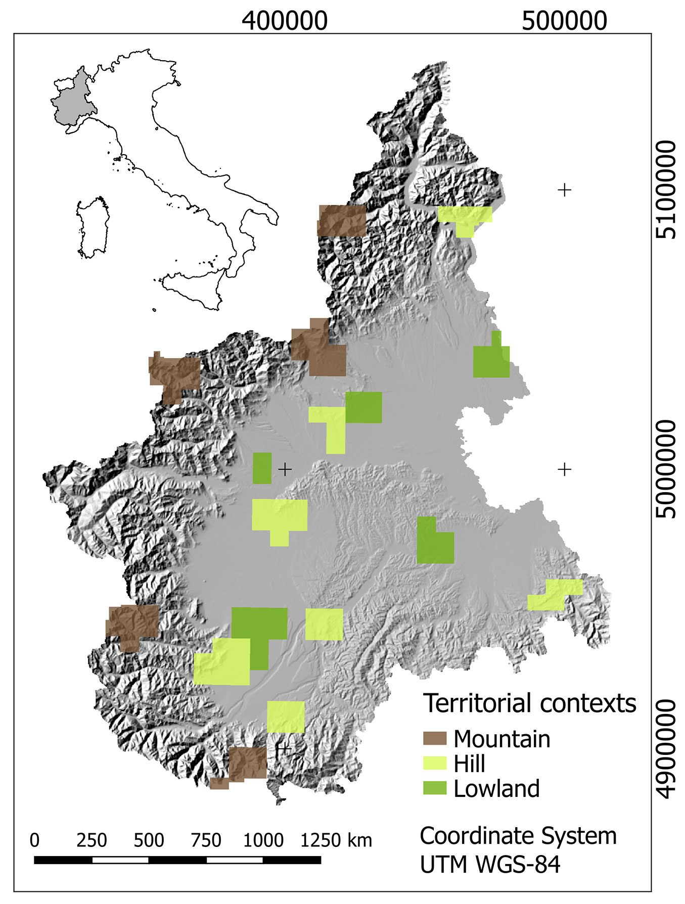
- Lowland context was represented by 24 tiles covering the following municipalities: Borgo d’Ale (4); Cameri (5); Venaria (2); Savigliano (8); Felizzano (5).
- Hill context was represented by 37 tiles covering the following municipalities: Verbania (6); Mazzè (4); Moncalieri (7); Busca (8) Villanova di Mondovì (4); Borghetto di Barbera (4); La Morra (4).
- Mountain context was represented by 35 tiles covering the following municipalities: Ceresole Reale (8); Macugnaga (6); Settimo Vittone/Carema/Chiaverano (8); Pontechianale (7); Limone Piemonte (6).
Several terrain characteristics of each landscape context are reported in Tab. 1.
Tab. 1 - Main terrain characteristics of the 3 landscape contexts considered, as inferred from sample tiles selected according to the administrative boundaries of the municipalities whose territory is mostly mountainous, hilly or flat. This determines the partial overlap of height and slope ranges among different contexts.
| Landscape contexts |
Area (ha) |
Height (m a.s.l.) | Slope (Degrees) | Roughness | ||
|---|---|---|---|---|---|---|
| Min-Max | Median | Min-Max | Median | Median | ||
| Lowland | 91100 | 92-442 | 231 | 0-16 | 0.97 | 16 |
| Hill | 134242 | 164-1622 | 343 | 0-43 | 5.90 | 56 |
| Mountain | 114446 | 225-4508 | 2108 | 0-72 | 21.60 | 336 |
CHM quality check
Co-registration (homology) of the DTM and the correspondent DSM tiles was tested to identify eventual pixel position displacement. Moreover, since many tiles showed local areas of missing values (“noData”), we tested if the number of regular (NOT-NULL) pixels was the same for DSM and correspondent DTM tiles. Statistics were then globally computed for all tiles representing the same landscape context.
CHM errors analysis
CHMs were computed by differencing DSMs and DTMs. As CHM values are expected to be positive or zero regardless of their geographic position, negative values were identified and assumed as proxies of potential CHM uncertainty. Error statistics were separately computed for each landscape context. Since the tolerance (double of precision) was assumed as a statistical measure of CHM uncertainty, statistics summarizing the occurrence of CHM negative values was called “a posteriori CHM tolerance” (τCHM). According to tolerance values of DTM (τDTM) and DSM (τDSM), it is also possible to estimate the expected CHM tolerance (hereafter: “a priori tolerance” - τCHM) by applying the Variance Propagation Law (VPL - [3]), as follows (eqn. 1):
Assuming that τDTM = τDSM, then (eqn. 2):
According to DTM and DSM metadata, τCHM was 0.83 m in the best case (τDTM = τDSM = 0.60 m) and 2.03 m in the worst case (e.g., mountain and forest areas), where τDTM = τDSM = 1.44 m. We assumed 0.83 (τCHM - the “best” tolerance) and 2.03 m (θCHM - the “worst” tolerance) as reference values to compare the CHM a posteriori tolerance with during our analysis.
CHM a posteriori tolerance estimation
For each of the 96 selected tiles, CHM was calculated from the correspondent gridded DTM and DSM. Negative CHM values (Δ-) were identified and the parameter p1 was computed to quantify the occurrence of CHM errors over images (eqn. 3):
where Nim is the total number of tile pixels and NΔ- is the number of CHM pixels with values < 0. The parameters p2 and p3 were also calculated as the percentages of CHM pixels (for each tested tile) where CHM error exceeds the expected tolerance thresholds (eqn. 4):
where NΔ-τCHM is the number of CHM pixels with Δ- < -τCHM; and (eqn. 5):
where NΔ- θCHM is the number of CHM pixels with Δ- < - θCHM. The reference statistical population in this case is NΔ- (i.e., all CHM negative values).
It is worth to notice that: (i) p1 certainly underestimates the actual occurrence of errors, since only negative errors are considered. Assuming that error frequency distribution is symmetric (i.e., error occurs equally with positive and negative sign), then p1 is expected to double; (ii) conversely, p2 and p3 are expected to be invariant even in the case the whole frequency distribution of errors is considered, since both the numerator and denominator of the ratio should double in this case.
Statistics regarding each tested tile were then averaged over each of the three reference landscape contexts. Since the parameters p1, p2 and p3 describe the frequency of significant CHM errors over the region, the statistic distribution of CHM errors was also computed considering all tiles regardless of possible map shifting and separately performed for each context.
CHM error vs. terrain morphometry
To investigate the relationship between CHM errors and landscape morphometry, a correlation analysis was carried out. First, a slope map (degrees) was computed from a low resolution (10×10 m) DTM available from the Regional cartographic office, using the Maximum Slope algorithm by Travis et al. ([26]) available in the software SAGA GIS. Scatterplots of CHM errors (absolute value) and the correspondent slope values were generated for each context. Due to the area morphology, slope values at CHM error locations were not equally distributed in their range of variability, thus affecting the reliability of the regression analysis. To solve this problem, 20 equally spaced slope classes were defined, and the mean absolute CHM error value (|m|) and the quantity |M| = |m| + 2σclass (where σclass is the standard deviation of the CHM errors falling in the considered slope class) were computed for each class. In this case, the parameter |m| is the average reference value of CHM uncertainty for each slope class, while |M| represents the “worst case” that can occur at each location. Assuming a normal distribution of CHM errors in each slope class, the 95.4 % of error absolute values are lower than |M|. Correlation and regression analysis were performed on both |m| and |M| separately in each landscape contexts. Since a strong correlation was found between slope and both |m| and |M|, two regressive models were used to estimate the potential CHM error at each location based on slope values. Models calibration was performed using all the available data (CHM errors) for each landscape context.
To further investigate the relationship between CHM errors and terrain morphology, spatial autocorrelation of CHM errors was analyzed using variograms in a sample tile (n. 190130) of the mountain context.
CHM error mapping
CHM error models of |m| and |M| previously calibrated for the mountain landscape context (the most critical) were used to map the potential CHM errors over the entire Piemonte Region. Modeling was performed using a slope map obtained from a coarser DTM dataset of Piemonte Region with a GSD (Ground Sample Distance) of 50 m. Pixels exceeding the best (τÌÂCHM) and the worst (θCHM) tolerance values were used to obtain the frequency distribution of height error over the whole region.
CHM error impact over forest categories
To assess the impact of CHM potential errors on the main regional forest categories, regional forest areas were identified using the FTC map obtained by the regional database. Twenty-one forest categories listed in FTC map were grouped in 12 classes according to Camerano et al. ([4]). We particularly focused on those areas where treeline potentially occurs (high altitude classes - 1500-2500 m a.s.l.).
Results
A preliminary check of co-registration of DTM and DSM tiles revealed that as much as 38.7 % of the sampled tiles was shifted. In all cases, the observed displacement was 0.5 pixel (2.5 m), indicating that the processing of georeferenced files by data producers was not rigorous. According to the producers’ metadata, DTM and DSM were separately managed during the production workflow, and this could have generated the observed tile translation, which unavoidably affects also the computation of CHM values.
Moreover, some unexpected differences between DSM and DTM were found. In fact, 44.8 % of the tested DSM tiles included a higher number of NOT-NULL pixels compared to the correspondent DTM tiles. These were mainly located along the map edges and were probably generated during the point cloud regularization step.
Tab. 2 reports the number of pixels of DSM exceeding the DTM ones for each landscape context, as well as their percentage over the entire regional territory and their equivalent area in hectars. These statistics were globally computed for all tiles belonging to the same landscape context. The results show that these areas represent a negligible part of the Piemonte Region, corresponding to 0.029%, 0.041% and 0.043% for lowland, hill and mountain contexts, respectively.
Tab. 2 - Counting of NOT-NULL pixels in the DSM and DTM sample tiles. The number of NOT-NULL pixels of DSM exceeding those of the corresponding DTM (D), their percentage over to the whole Piemonte Region area, and their equivalent surface in hectares are reported. Statistics were globally computed for all tiles belonging to the same landscape context.
| Landscape contexts |
D (n. pixels) |
Area (%) |
ha |
|---|---|---|---|
| Lowland | 10813 | 0.029 | 27.0 |
| Hill | 23825 | 0.041 | 59.5 |
| Mountain | 20197 | 0.043 | 50.4 |
CHM error analysis
Since a significant number of DTM and DSM tiles were found to be not properly co-registered, CHM error analysis was separately performed for “matching” and “shifted” tiles in each landscape context. The percentages p1, p2 and p3 (eqn. 3-5) were then computed for each of the two groups (Tab. 3). Results showed that the percentage of negative CHM values significantly different from zero was not negligible, especially in mountain areas. Moreover, a higher percentage of errors (i.e., lower accuracy) was found where spatial displacement between DTM and DSM was observed (shifted tiles). Significant CHM errors in the mountain context increased from about 4.4% for matching tiles up to 29.3% for shifted tiles. It is worth to stress that this situation only concerns this specific release of data we tested, which can be easily corrected by revising the processing workflow. We therefore chose as the most appropriate value for τÌÂCHM that observed for the “matching” subset. Additionally, such percentages could even be as much as twice the above figures, since the CHM errors considered in this study may theoretically represent only the half of the whole error distribution (i.e., the negative errors), as already mentioned.
Tab. 3 - CHM error occurrences for the tested tiles, calculated by averaging the parameters p1, p2, p3 of tiles belonging to the same landscape context (lowlands, hill and mountain).
| Tiles | Landscape contexts |
p1
|
p2
|
p3
|
|---|---|---|---|---|
| Matching | Lowland | 0.63 | 13.58 | 1.32 |
| Hill | 0.29 | 13.21 | 3.58 | |
| Mountain | 4.41 | 30.41 | 9.30 | |
| Shifted | Lowland | 0.92 | 0.47 | 0.03 |
| Hill | 2.25 | 15.06 | 5.47 | |
| Mountain | 29.30 | 58.94 | 20.48 |
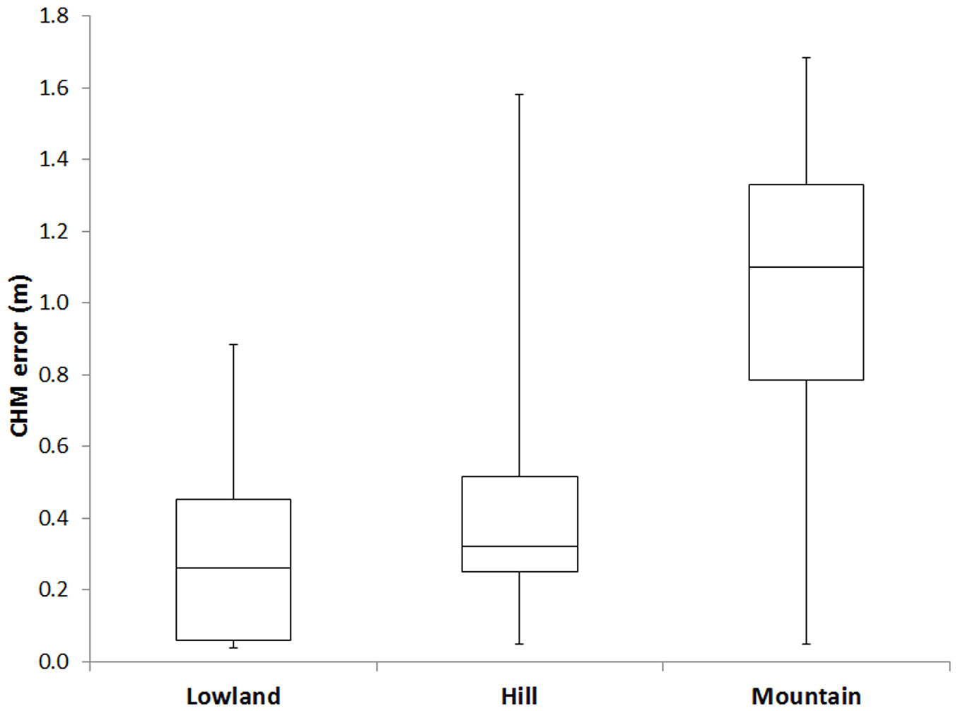
The statistic distribution of the observed CHM errors for each context is summarized in Fig. 2. CHM errors showed an increasing trend from lowlands (0.04 m, 0.26 m and 0.89 m for minimum, median and maximum values, respectively) to hills (0.05 m, 0.32 m and 1.58 m, respectively) and to mountains (0.05 m, 1.10 m and 1.68 m, respectively), suggesting a strong dependency of errors from topography.
Fig. 2 - Boxplots of the CHM error distribution for lowland, hill and mountain contexts. The ends of whiskers represents the maximum and minimum values of the distribution.
CHM error s. terrain morphometry
Fig. 3 - Correlation of CHM errors with slope. (a-e) Frequency distribution of CHM errors in slope classes for hill (a) and mountain (e) contexts. (b-f) Regression analysis of slope versus |m| and |M| statistics for hill (b) and mountain (f) contexts. (c, d, g, h) Scatterplots of the observed vs. predicted values of |m| (c, g) and |M| (d, h) for the hill (c, d) and mountain (g, h) contexts.
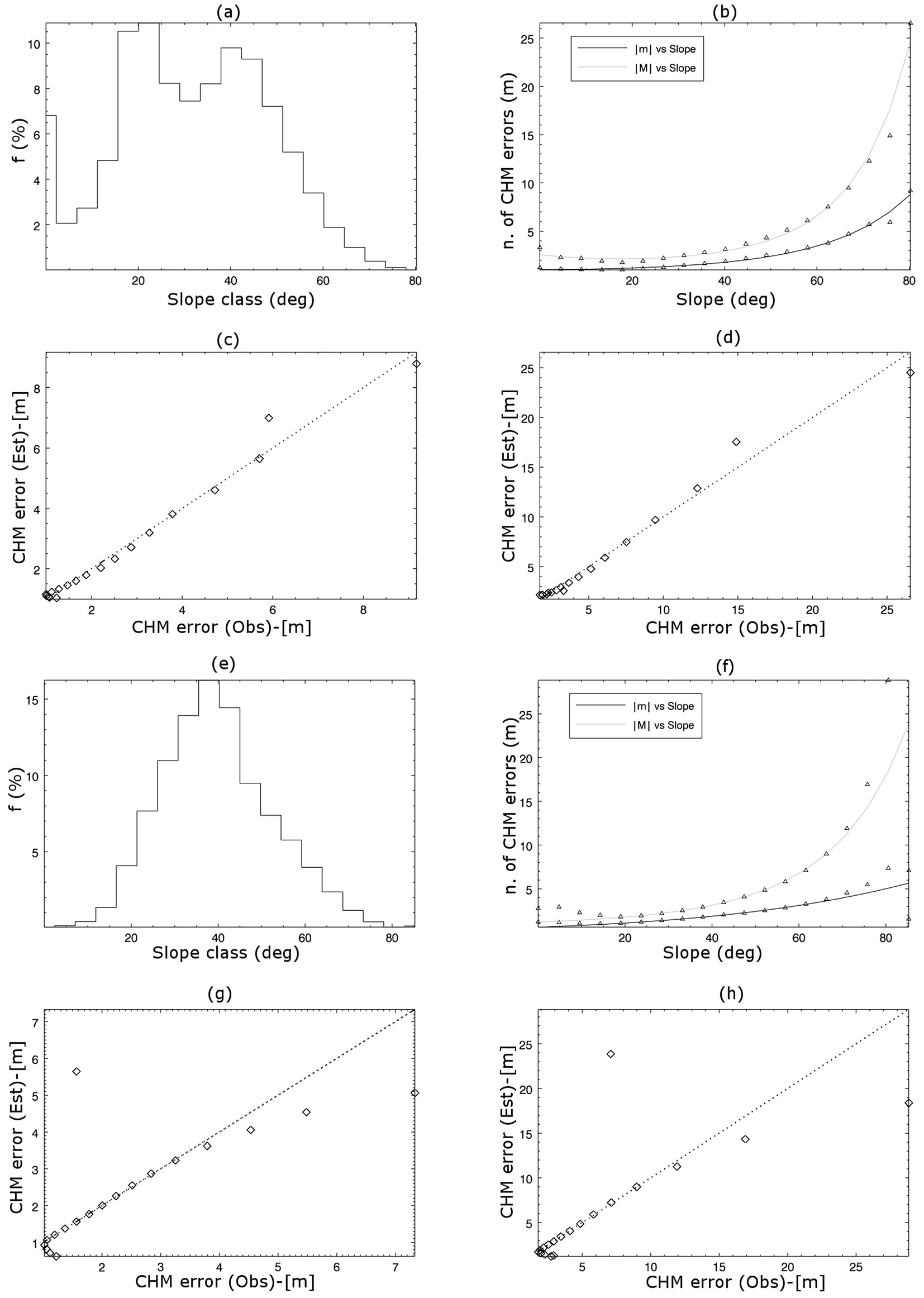
As not negligible CHM errors were recorded in mountain and hilly areas, their dependence from terrain slope was tested. Scatterplots of slope vs. both |m| and |M| revealed a strong correlation between these variables in both hill and mountain contexts (Fig. 3b, Fig. 3f). The following exponential regression model showed the best fitting to the observed data (eqn. 6):
where ε is the mean (|m|) or worst (|M|) CHM error (m), depending on the modeled parameter, and β is the local slope angle (degrees). In flat areas, β is zero, thus eqn. 6 can be rewritten as |ε| = expa. The values of parameters a, b, and c obtained by fitting the above model in both hill and mountain contexts are reported in Tab. 4.
Tab. 4 - Pearson’s correlation coefficients (R) and parameters values (a, b, c) of the regression model (eqn. 6) used to predict CHM error (|m| and |M|) based on slope values in the mountain and hill contexts.
| Parameters | Mountain | Hill | ||
|---|---|---|---|---|
| |m| vs. Slope | |M| vs. Slope | |m| vs. Slope | |M| vs. Slope | |
| R | 0.84 | 0. 90 | 0.99 | 0.99 |
a
|
-0.47969 | 0.19952 | 0.02842 | 0.94374 |
b
|
0.02911 | 0.01335 | 0.00077 | -0.02155 |
c
|
-0.00007 | 0.00028 | 0.00028 | 0.00065 |
Fig. 3 reports the results of the correlation analysis between CHM errors and slope. A strong significant relationship was found, with error values increasing with slope in both hill and mountain contexts. Trends of the parameters |m| and |M| were similar in shape and value for both contexts, though the coefficients of the regression model were slightly different. This could be explained by the different statistical distribution of the CHM errors across slope classes.
To better explore the dependence of CHM errors from slope, a mountain sample tile (n. 190130) was chosen and a random sample of its CHM errors (20 % of the total) was extracted. Selected points were differently colored according to CHM error value and superimposed over the correspondent DTM tile (left panel of Fig. S1 - Supplementary material). Map showed that the majority of CHM errors mainly occurred in those parts of the area analyzed where topography is highly variable and the elevation is high. Moreover, the cumulative frequency distributions of slope and height values corresponding to CHM negative pixels showed that 100% of errors occurred at elevations higher than 1300 m a.s.l., even if height values of the area ranged between 280 and 2900 m a.s.l. (Fig. S1, right panel). This confirms the strong correlation of CHM error with slope, but not with elevation.
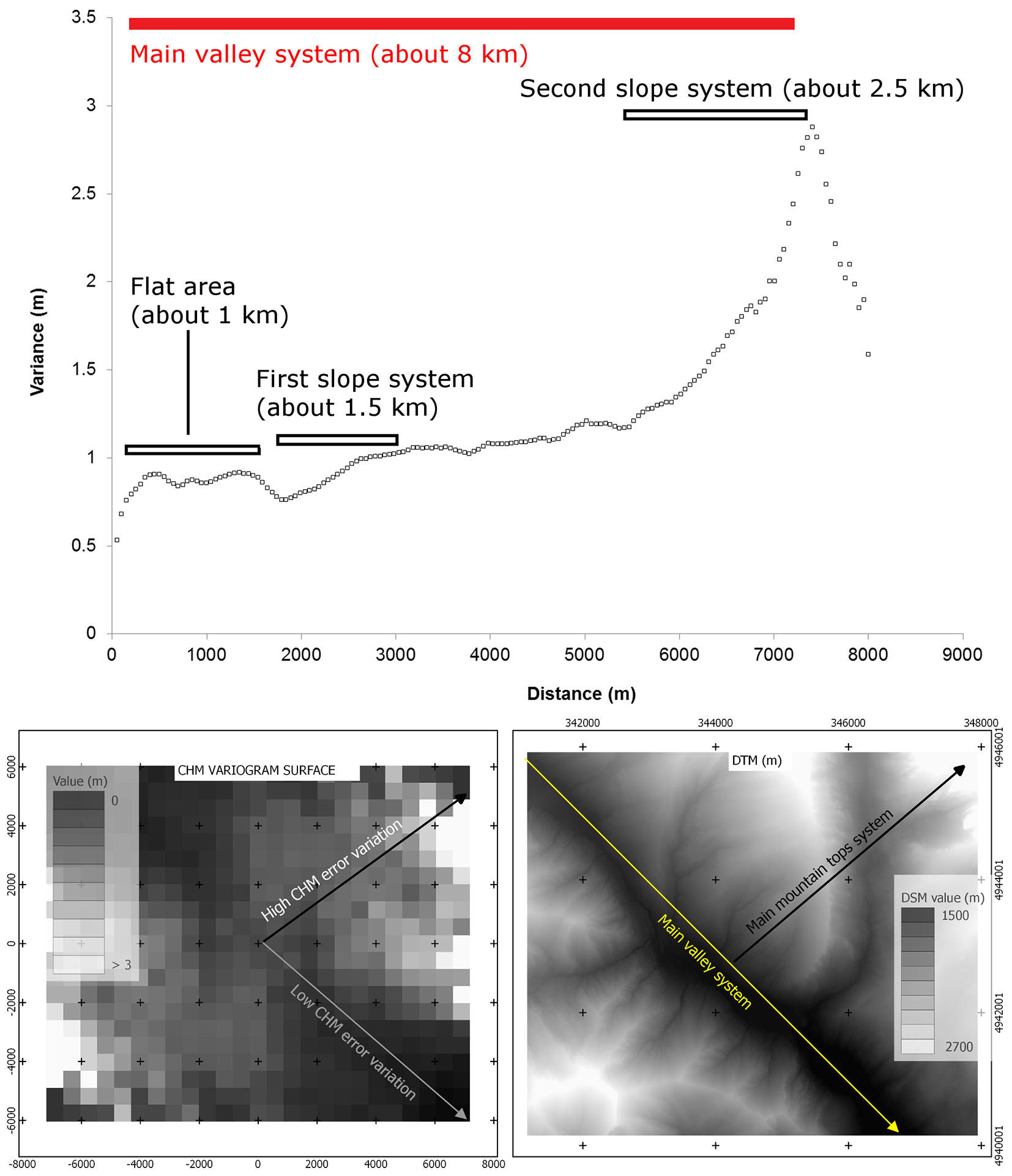
Spatial autocorrelation analysis was applied to the sample tile previously used for the error distribution analysis (n. 190130). As displayed by the variogram reported in Fig. 4, CHM error variance did not result distance-dependent (no spatial autocorrelation) at the closest distances (up to 1.5 km), while it markedly increased up to 7.5 km and then decreased for further distances. Furthermore, a bidimensional (surface) variogram generated for the same tile clearly showed that error variation was higher along the SW-NE direction (lower left panel in Fig. 4), i.e., along the main elevation gradients in the area (lower right panel). Contrastingly, CHM error variance was slowly decreasing along the direction of the main valley system (NW-SE), further confirming the strong CHM error dependency from geomorphology.
Fig. 4 - Variogram and surface variogram of CHM errors for sample tile no. 190130. (Upper panel): spatial autocorrelation of CHM errors, reflected by the increase of error variance with distance, indicating that morphology is a conditioning factor. The distance range (approx. 8 km) was consistent with the length of the main valley system (red bar). Sub-patterns of variation within this distance can be related to the local morphology (black bars). (Lower panels): bidimensional (surface) variogram of CHM errors (left) and the corresponding DTM (right). Error variation was weak along the flat area (valley), while increased on steep slopes.
CHM error mapping
Modeling of the dependence of CHM errors from terrain morphology allowed to map the CHM potential error over the whole regional territory. A potential CHM error map with cell size of 50×50 m was generated using the mountain context parameters for both |m| and |M| in eqn. 5. To this goal, a slope map was generated from a 50×50 m available DTM covering the entire region.
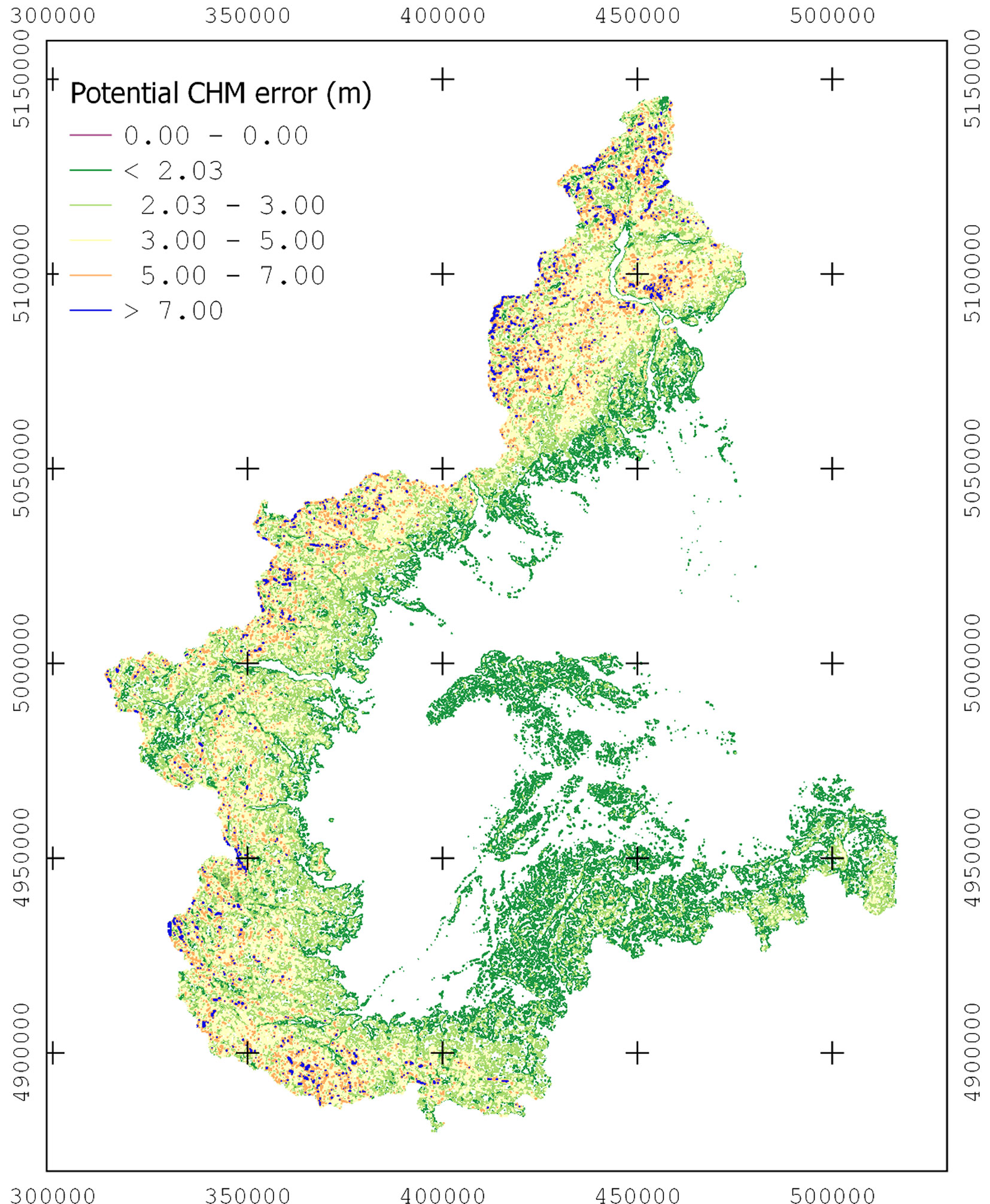
Fig. 5 shows the distribution of CHM error (|M|) over the Piemonte Region. Significant |M| error values (> 3 m) were found only in the hill or mountain contexts. The expected mean CHM error (|m|) was generally consistent with the declared accuracy of the DTM, and consequently of the DSM (Tab. 5). Indeed, |m| values were lower than the expected “best” tolerance (0.83 m) in 51% of the mapped territory, while in the remaining part |m| values were lower than the “worst” tolerance (2.03 m). Moreover, |M| errors were surprisingly low, being smaller than the “worst” tolerance (2.03 m) in about 80% of the region. Hence, 20% of the regional territory (mainly located on mountains) suffers from a high CHM uncertainty.
Fig. 5 - Map of the potential CHM |M| error distribution in the Piemonte Region. Significant |M| error values (> 3 m - yellow, orange and blue pixels) were found only in the hill and mountain contexts.
Tab. 5 - CHM errors distribution in the Piemonte Region, expressed as percentage of the regional area falling within the considered CHM error (|m| and |M|) classes.
| CHM error (m) | Area (%) |
|
|---|---|---|
| |m| | |M| | |
| < 0.83 | 51 | 0 |
| 0.83 - 1.66 | 40 | 65 |
| 1.66 - 2.03 | 5 | 14 |
| 2.03 - 3.00 | 2.6 | 16 |
| 3.00 - 4.00 | 0.4 | 4 |
| 4.00 - 6.00 | 1 | 0.8 |
| > 6.00 | 0 | 0.2 |
Regarding the treeline, an additional analysis was carried out to verify how CHM potential errors might affect treeline detection at high elevations (1500-2500 m a.s.l.). Six elevation classes were defined and mapped using the available DTM (Tab. 6), and the potential CHM errors were computed for each class using the CHM error map obtained above. Only the values of |m| and |M| above 2.03 m were considered in this analysis, as the minimum height of trees forming the treeline is commonly considered to be 2 m. The majority of not negligible CHM potential errors were found in the elevation class where the treeline commonly occurs (1500-2500 m a.s.l. - Tab. 6). We concluded that the use of the LiDar dataset tested in this study could not be suitable for studies on local treeline dynamics and variation. Some improvement could be attained by combining the CHM information with the digital orthoimages acquired during the same flight (ICE aerial-photogrammetric survey 2009-2011).
Tab. 6 - Mean (|m|) and maximum (|M|) potential CHM error calculated for six elevation classes in the Piemonte Region. Values are mean (± standard deviation) of |m| and |M| values higher than 2.03 m (the “worst” tolerance).
| Elevation class (m a.s.l.) |
|m| Area (ha) |
|M| Area (ha) |
|m| value (m) |
|M| value (m) |
|---|---|---|---|---|
| 0-150 | 0 | 0 | 0 | 0 |
| 150-300 | 0 | 0 | 0 | 0 |
| 300-700 | 81.25 | 10637.50 | 2.30 ± 0.21 | 2.38 ± 0.33 |
| 700-1500 | 3468.75 | 137350.00 | 2.31 ± 0.28 | 2.47 ± 0.46 |
| 1500-2500 (treeline) | 10181.25 | 219418.75 | 2.33 ± 0.33 | 2.55 ± 0.58 |
| > 2500 | 6525.00 | 49206.25 | 2.46 ± 0.46 | 2.85 ± 1.35 |
Impact of CHM error on forest categories
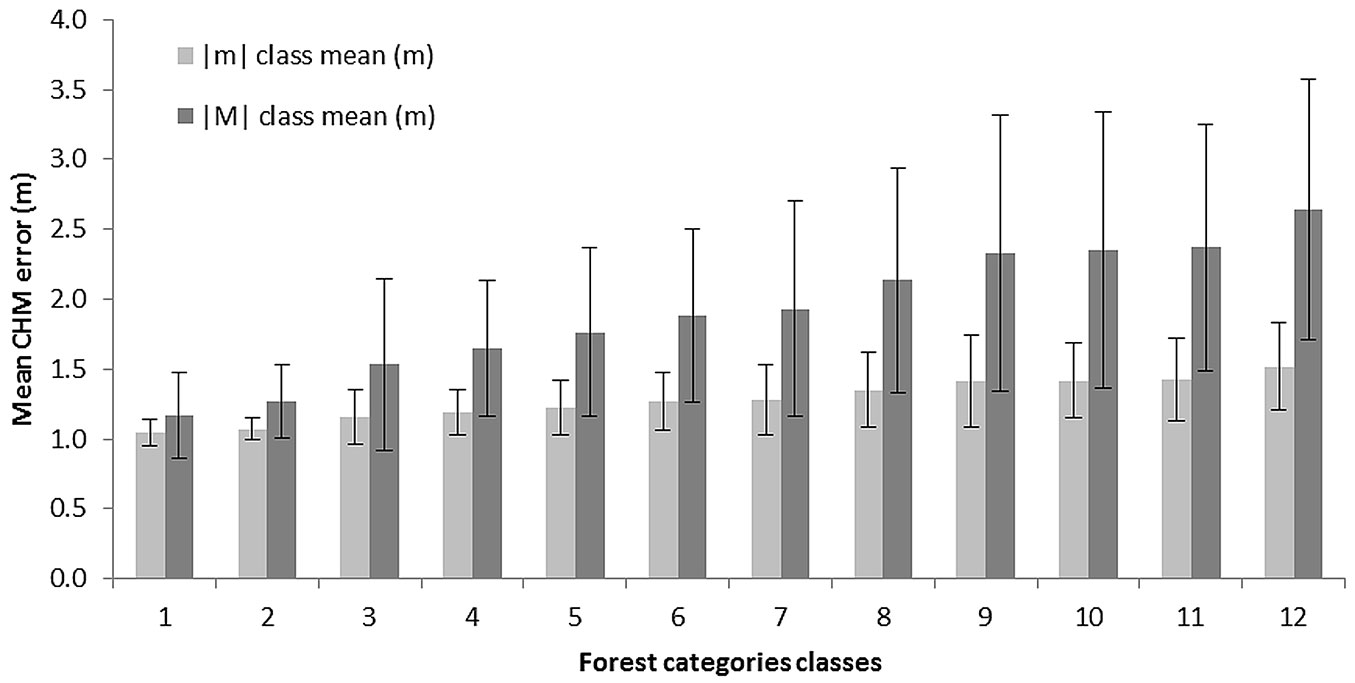
CHM potential error was related to forest areas using the available FTC vector map described above. Polygon zonal statistics (mean and standard deviation of |M| values, average values of slope in degrees, elevation and covered area in %) were calculated for 12 forest categories representing the main forest types of Piemonte. Main CHM statistics obtained are reported in Tab. 7, while Fig. 6 reports the mean and standard deviation values of |m| and |M| for each category, sorted by the mean value of class slope (from the lowest to the highest). A strong linear correlation (R2 = 0.8774, p<0.01) was found between the standard deviation of |m| and slope, suggesting that not only CHM potential error increases with slope, but also local uncertainty of its estimation. Since the highest CHM errors were observed not only where slope is higher but also at the highest elevations, the relationship between elevation and slope for the whole region was tested using an exponential regression model on the average values for each forest categories and. Results showed a strong relationship between the variables considered (R2 = 0.9007, p<0.01).
Tab. 7 - CHM error statistics for 12 forest categories representing the main forest types of the Piemonte Region, sorted by increasing value of mean slope in each category. Mean values (± standard deviation) of potential CHM errors |m| and |M| are reported.
| Forest category | |m| (m) |
|M| (m) |
Slope (degrees) |
Elevation (m s.l.m.) |
Area (%) |
|---|---|---|---|---|---|
| Riparian willow and poplar forest | 1.03 ± 0.09 | 1.20 ± 0.32 | 5.35 | 173.86 | 1.51 |
| Black Locust forest | 1.08 ± 0.08 | 1.25 ± 0.25 | 8.51 | 276.85 | 12.87 |
| Sessile oak, Oak-Hornbeam and Turkey oak forests | 1.13 ± 0.19 | 1.54 ± 0.62 | 13.54 | 352.29 | 8.07 |
| Downy oak and Hop-Hornbeam forests | 1.18 ± 0.16 | 1.67 ± 0.50 | 17.21 | 273.97 | 6.41 |
| Chestnut forest | 1.24 ± 0.21 | 1.75 ± 0.60 | 18.94 | 583.77 | 23.66 |
| Conifer tree plantation | 1.26 ± 0.21 | 1.91 ± 0.64 | 21.13 | 768.06 | 2.30 |
| Mesophilous mixed broad-leaves forest | 1.30 ± 0.26 | 1.92 ± 0.76 | 21.26 | 925.03 | 4.30 |
| Scots pine, Mountain pine and Cluster pine forests | 1.37 ± 0.29 | 2.10 ± 0.79 | 24.53 | 1040.60 | 1.65 |
| Mixed broad-leaves pioneer forest and shrub forest | 1.40 ± 0.31 | 2.28 ± 0.98 | 26.53 | 1214.90 | 11.91 |
| Beech forest | 1.43 ± 0.29 | 2.33 ± 0.80 | 27.87 | 1126.46 | 14.75 |
| Larch and Arolla pine forest | 1.45 ± 0.31 | 2.36 ± 0.87 | 27.94 | 1723.87 | 9.68 |
| Silver fir and Spruce forests | 1.50 ± 0.33 | 2.67 ± 0.94 | 31.40 | 1433.78 | 2.89 |
Fig. 6 - Mean values (± standard deviation) of potential CHM errors (|m| and |M|) for 12 forest categories representing the main forest types of the Piemonte Region, sorted by their mean slope value (lowest to highest). (1): Riparian willow and poplar forest; (2): black locust forest; (3): sessile oak, oak-hornbeam and Turkey oak forests; (4): Downy oak and hop-hornbeam forests; (5): chestnut forests; (6): conifer tree plantations; (7): mesophilous mixed broad-leaves forest; (8): Scots pine, Mountain pine and Cluster pine forests; (9): mixed broad-leaves pioneer forest and shrub forest; (10): beech forest; (11): larch and Arolla pine forest; (12): silver fir and spruce forests.
Discussion
In this study, we evaluated the quality of the CHM obtained from the LiDAR dataset (gridded DSM and DTM) provided by the Piemonte Region using an indirect method based on the assessment of internal anomalies affecting CHM data. The proposed method provides a fast evaluation of data uncertainty, with no direct ground validation required.
We estimated the local potential CHM error and demonstrated that it is strictly dependent from slope. The relationship between CHM error and slope was independently modeled for mountain, hill and flat terrain contexts by exponential regression. Using the model calibrated on the mountain context, the local CHM potential error was estimated and mapped over the whole region. This analysis showed that the mean potential error (|m|) was lower than the nominal best tolerance (0.83 m) over 51% of the territory, while the maximum potential CHM error (|M|) was lower than the nominal worst tolerance (2.03 m) in about 80% of the analyzed region. However, CHM uncertainty was not negligible (2.33-2.55 m) at the highest elevations (1500-2500 m a.s.l.), including the treeline.
Regarding the impact of CHM errors on different forest types, we found that the mean potential error is almost forest class-independent as for both class mean value and standard deviation (1.10-1.45 m), which instead increased with slope when the maximum potential CHM error is considered. Nonetheless, the values reported in Tab. 7 could be advised as reference estimates of |m| and |M| for each forest category. However, when used in forest application, it should be taken into consideration that (i) the reported values depend on the prevailing morphology of the area considered (slope) and not on forest species; and (ii) most forest categories show negligible CHM errors as compared with the “worst” declared accuracy of the parent datasets. This makes the LiDAR gridded datasets of the Piemonte Region suitable for forest applications for most of the regional territory. However, the steepest and highest elevation areas (about 20% of the regional territory) suffer from non-negligible errors, making the measurements of tree height derived from CHM not fully reliable. In particular, the use of the tested CHM seems to be inappropriate for treeline mapping purposes, as unreliable results might be obtained. Indeed, according to our results, the potential CHM error detected for such elevation class is fully consistent with the minimum height of trees forming the treeline (2-5 m - [11]).
It is worth to notice that the gridded DTM tested in this study is established and proven by the Piemonte Region, while the gridded DSM used is not an official release yet, and therefore it could be improved by revising the original point cloud of the LiDAR acquisition. DTM, however, can be freely downloaded from the official Geoportal website of the Piemonte Region.
The main goal of this study was to provide users with an easy tool (the model relating CHM error and slope) for assessing the potential CHM error to be adopted in customized forest applications. To this end, we recommend particular caution when mountain forest areas are included in the study, as steep slopes may strongly decrease the vertical accuracy issued with the original LiDAR acquisition, and consequently vertical errors may increase.
Future research will be addressed to assess the uncertainty of wood volume and biomass estimation from LiDAR CHM values. This could be obtained by reversing ordinary empirical models of volume estimation, using tree height as predictor and stem diameter as the predicted value. To this purpose, CHM uncertainty has to be propagated along the model to obtain the potential error for stem diameter, and consequently of the error affecting biomass or wood volume estimates.
Acknowledgements
The authors are grateful to Gian Bartolomeo Siletto and Stefano Campus of the Cartography and GIS department of the Piemonte Region (Department of Land Governance and Protection) for providing the dataset and the metadata used in this study.
References
Gscholar
Gscholar
Online | Gscholar
Gscholar
CrossRef | Gscholar
Gscholar
Authors’ Info
Authors’ Affiliation
Vanina Fissore
Andrea Lessio
Renzo Motta
DISAFA, University of Torino, l.go Paolo Braccini 2, I-10095, Grugliasco, TO (Italy)
Corresponding author
Paper Info
Citation
Borgogno Mondino E, Fissore V, Lessio A, Motta R (2016). Are the new gridded DSM/DTMs of the Piemonte Region (Italy) proper for forestry? A fast and simple approach for a posteriori metric assessment. iForest 9: 901-909. - doi: 10.3832/ifor1992-009
Academic Editor
Matteo Garbarino
Paper history
Received: Jan 21, 2016
Accepted: May 13, 2016
First online: Aug 29, 2016
Publication Date: Dec 14, 2016
Publication Time: 3.60 months
Copyright Information
© SISEF - The Italian Society of Silviculture and Forest Ecology 2016
Open Access
This article is distributed under the terms of the Creative Commons Attribution-Non Commercial 4.0 International (https://creativecommons.org/licenses/by-nc/4.0/), which permits unrestricted use, distribution, and reproduction in any medium, provided you give appropriate credit to the original author(s) and the source, provide a link to the Creative Commons license, and indicate if changes were made.

Web Metrics
Breakdown by View Type
Article Usage
Total Article Views: 49352
(from publication date up to now)
Breakdown by View Type
HTML Page Views: 41084
Abstract Page Views: 2971
PDF Downloads: 3967
Citation/Reference Downloads: 48
XML Downloads: 1282
Web Metrics
Days since publication: 3607
Overall contacts: 49352
Avg. contacts per week: 95.78
Article Citations
Article citations are based on data periodically collected from the Clarivate Web of Science web site
(last update: Mar 2025)
Total number of cites (since 2016): 11
Average cites per year: 1.10
Publication Metrics
by Dimensions ©
Articles citing this article
List of the papers citing this article based on CrossRef Cited-by.
Related Contents
iForest Similar Articles
Review Papers
Analysis of full-waveform LiDAR data for forestry applications: a review of investigations and methods
vol. 4, pp. 100-106 (online: 01 June 2011)
Review Papers
Accuracy of determining specific parameters of the urban forest using remote sensing
vol. 12, pp. 498-510 (online: 02 December 2019)
Review Papers
Remote sensing-supported vegetation parameters for regional climate models: a brief review
vol. 3, pp. 98-101 (online: 15 July 2010)
Research Articles
Assessing water quality by remote sensing in small lakes: the case study of Monticchio lakes in southern Italy
vol. 2, pp. 154-161 (online: 30 July 2009)
Research Articles
High resolution biomass mapping in tropical forests with LiDAR-derived Digital Models: Poás Volcano National Park (Costa Rica)
vol. 10, pp. 259-266 (online: 23 February 2017)
Review Papers
Remote sensing of selective logging in tropical forests: current state and future directions
vol. 13, pp. 286-300 (online: 10 July 2020)
Research Articles
Identification and characterization of gaps and roads in the Amazon rainforest with LiDAR data
vol. 17, pp. 229-235 (online: 03 August 2024)
Research Articles
Classification of xeric scrub forest species using machine learning and optical and LiDAR drone data capture
vol. 18, pp. 357-365 (online: 07 December 2025)
Research Articles
Estimation of aboveground forest biomass in Galicia (NW Spain) by the combined use of LiDAR, LANDSAT ETM+ and National Forest Inventory data
vol. 10, pp. 590-596 (online: 15 May 2017)
Research Articles
Mapping the vegetation and spatial dynamics of Sinharaja tropical rain forest incorporating NASA’s GEDI spaceborne LiDAR data and multispectral satellite images
vol. 18, pp. 45-53 (online: 01 April 2025)
iForest Database Search
Search By Author
Search By Keyword
Google Scholar Search
Citing Articles
Search By Author
Search By Keywords
PubMed Search
Search By Author
Search By Keyword


