Analysis of full-waveform LiDAR data for forestry applications: a review of investigations and methods
iForest - Biogeosciences and Forestry, Volume 4, Issue 3, Pages 100-106 (2011)
doi: https://doi.org/10.3832/ifor0562-004
Published: Jun 01, 2011 - Copyright © 2011 SISEF
Review Papers
Abstract
The goal of this review is to present leading examples of current methodologies for extracting forest characteristics from full-waveform LiDAR data. Four key questions are addressed: (i) does full-waveform LiDAR provide advantages over discrete-return laser sensors; (ii) will full-waveform LiDAR provide valid results in support of forest inventory operations and allow for a decrease in ground sampling efforts; (iii) is the use of full-waveform LiDAR data cost effective; and (iv) what is the scope of the applied methods (i.e., is full-waveform LiDAR accurate for different forest compositions, structures, and densities, and is it sensitive to leaf-off/leaf-on conditions)? Key forest structure characteristics can be estimated with significant accuracy using full-waveform metrics, although methodologies and their corresponding accuracies differ. For example, some processing methods are valid at the plot scale, whereas other procedures perform well at the regional scale; to be effective, certain LiDAR data analyses require a minimum point density, whereas other methods perform well using large-footprint sensors. Therefore, it is important to match processing methods with the appropriate scale and scope. The aim of this paper is to provide the forest research community and remote sensing technology developers with an overview of existing methods for inferring key forest characteristics, including their applicability and performance.
Keywords
LiDAR, Full-waveform, Forest metrics, Forest structure parameters, Active remote sensing
Introduction
One long-standing objective of forest ecosystem remote sensing has been to provide methods for extracting metrics of interest with equal or better accuracy than ground-based forest inventory methods. The use of remote sensing technologies is expanding due to an increasing need to collect data to model complex environmental dynamics (see [10] for a comprehensive overview). Digital image analysis, a classic remote sensing application, has been used for decades for forest mapping and inventory evaluations, and it has played a substantial role in forest monitoring and assessment ([6]). LiDAR (light detection and ranging), a relatively recent type of remote sensing, uses laser-pulse time-of-flight data to measure distances and corresponding back-scatter intensities. It has been demonstrated that LiDAR can provide accurate estimations of many key forest characteristics. For example, canopy height, topography and vertical distribution can be directly retrieved from LiDAR data; above-ground biomass, average basal area, average stem diameter and canopy volume can be modeled; and leaf area indices and canopy cover can be inferred by combining LiDAR and optical sensor data ([8]). Results based on the integration of LiDAR and hyperspectral digital image data sources have been shown to be superior to results obtained using a single data source ([22]). Developments in sensor technology over the past ten years have led to the option of equipping airborne LiDAR systems with full-waveform (FW) sensors. These sensors are called “full-waveform” because laser pulses that are returning to the sensor after being back-scattered by objects on the Earth’s surface (e.g., canopy, ground and water) are sampled at regular time intervals. Therefore, substantially more information is recorded and stored using FW LiDAR relative to discrete-return LiDAR. LiDAR laser pulses project a footprint on the Earth’s surface (some authors prefer the term “diffraction cone” to emphasise the 3D aspect, e.g., [19]) that can vary in size from a few centimeters to several meters depending on beam divergence and flight height. FW sensors are categorized as having either a large or small laser footprint size, which determines the size of an area sampled by a single pulse. The resulting waveform is representative of the forest structure within an area because it is “shaped” by the properties of all elements that intersect the beam path; for example, in an area with forest cover, these elements would be, from top to bottom, the canopy surface, the crown volume, the understory layer and the ground surface. FW LiDAR has provided improved height estimations ([9]), point density measurements ([5]) and range determinations ([32]) over discrete-return LiDAR methods.
The objective of this review is to provide an outline of current methods that have been used successfully for extracting key forest information from FW LiDAR data. This paper is divided into the following sections: an overview of FW characteristics, a description of common pre-processing steps, a discussion of tree-scale and plot-scale methods and a final tabular summary of highlights (Tab. 1).
Tab. 1 - Highlights of experimental results from full-waveform LiDAR applications in forestry. (*): single tree scale; (§): small footprint, plot-scale; (#): large footprint, plot-scale.
| Scale | Authors | Key-line of method | Main results |
|---|---|---|---|
| * | Reitberger et al. (2007) | Improve tree position detection by modelling stem | 61% and 41% detection rate respectively for coniferous and deciduous. |
| * | Reitberger et al. (2008) | Tree features computed from the 3-dimensional coordinates of the reflections, the intensity and the pulse width are used to detect coniferous and deciduous trees by an unsupervised classification | 85% and 96% accuracy respectively for leaf-on and leaf-off conditions in distinguishing coniferous from deciduous. |
| * | Reitberger et al. (2009a) | Use Normalized cut segmentation - based on voxel space - plus unsupervised classification to detect trees. | Improved classification by 12% compared to common watershed algorithm. |
| * | Reitberger et al. (2009b) | Use Normalized cut segmentation and unsupervised classification based on waveform metrics to detect single trees also in lower layer. | Best classification 93% of trees, also in lower layer, point density very little impact. |
| § | Wagner et al. (2008) | Decision tree classification using number of return peaks, width and amplitude information. | Kappa coefficient of concordance = 0.8 in stand segmentation. |
| § | Rossmann et al. (2009) | Integrate FW LiDAR with SPOT - aerial image analysis for stand segmentation and characterization using decision tree, object-oriented classification. | 2.8% error on overall volume estimation. |
| § | Chauve et al. (2008) | Additional point detection from weak echoes -using advanced peak detection and modelling - improves height estimation and increases the amount of information on lower storey. | 5 cm improvement of bias and standard deviation in CHM compared to discrete-return LiDAR. |
| # | Drake et al. (2002) | Several metrics describing vertical distribution of forest structure are derived from the waveform of return pulse to infer key parameters. | Quadratic mean BHD, ABA and AGBM had significant correlation values of 0.93, 0.72 and 0.93 respectively. |
| # | Anderson et al. (2008) | AGBM information estimated from LiDAR integrated with digital image analysis to extract quadratic mean BHD, ABA and AGBM. | 8-9% improvement in correlation and a decrease of 5-8% in error |
| # | Harding et al. (2001) | Canopy height profiling by processing the waveform to extract height distribution of canopy closure from waveform. | ground-measured and LiDAR -estimated CHP correlation of: young (0.75), intermediate (0.52) mature (0.33) and old-growth (0.43). |
| # | Lefsky et al. (2002), Lefsky et al. (2005) | Three different biomes (2002) and five different contexts in same biome (2005) tested for quality of estimation of LAI and AGBM. | AGBM correlation value of 0.84 over biomes with general equation. Best LAI and AGBM 0.81 and 0.92 respectively. Regional scale validity. |
| # | Means et al. (1999) | Interactive graphical and regression techniques used for modelling forest characteristics with FW LiDAR metrics over coniferous forest. | Height, basal area, total biomass and leaf biomass R2 of 0.95, 0.96, 0.96, and 0.84, respectively. |
Full-waveform characteristics and pre-processing methods
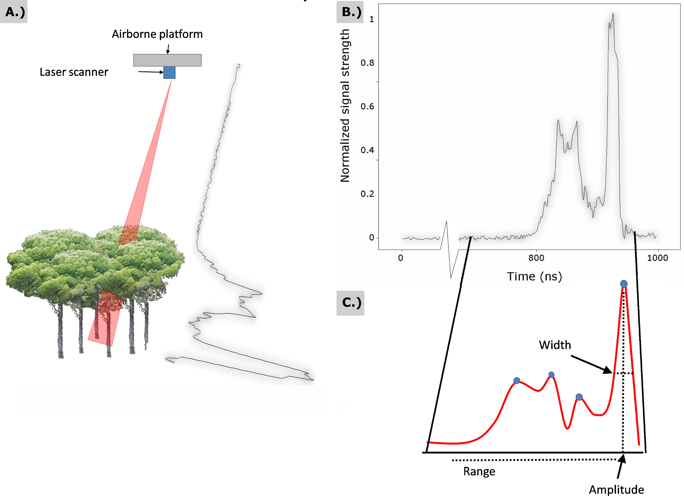
Unlike discrete-return laser systems, full-waveform LiDAR samples and records the entire back-scattered signal intensity (Fig. 1) at regular time intervals (typically ~1 ns). Laser pulse data are typically registered in a geographic reference frame using GPS (Global Positioning System) and IMU (inertial measuring unit) data obtained from positioning and orientation sensors, respectively, located within the aircraft.
Fig. 1 - (A) Schema of a full-waveform return signal from forested cover; (B) plot of digitizer counts as a function of time; (C) modeled waveform where each peak is characterized by a range, width and amplitude.
Depending on the sampling frequency, the vertical resolution of a waveform can vary. For example, many systems sample once every 1 ns (a frequency of 1GHz), which corresponds to a vertical resolution of 15 cm according to the following equation (eqn. 1):
where c is the average speed of light in atmosphere, t is time in seconds, and d is the distance traveled by light.
Signal pre-processing is used to normalize LiDAR information and to decrease or eliminate any element that can be a source of error in further processing steps (i.e., noise, outliers or emitted signal shape). Normalization is performed by dividing the single return energy from the total received energy such that the integral of the waveform is equal to one. Return energy is not constant for all return events; therefore, normalization allows for the comparison of absolute pulse shapes. Noise is abated by calculating a threshold value based on the mean and variance of intensity for a segment of the signal where only noise is present (before any reflecting element); only an intensity above this threshold value can be considered significant ([7]). The entire signal can be smoothed to decrease the noise content using filters, such as the Weiner filter ([13]). Finally, to obtain the surface response independent from the transmitted pulse, a deconvolution can be applied to the incoming waveform shape ([13]). This deconvolution is necessary in cases where the transmitted pulse is irregular and differs between laser shots.
After pre-processing, a waveform can be parametrized to extract peak data by recording the corresponding peak amplitude, width and range index of the peak maximum. Waveform peaks correspond to surface elements that were intercepted by the laser pulse. A common method for peak detection is Gaussian decomposition ([13]), which is used to fit a generalized Gaussian function according to the Levenberg-Marquardt algorithm ([31]). Other functions for detecting the peaks have been tested, and several methods have been found to improve results under certain conditions ([4]).
Further details on full-waveform analysis can be found in the existing literature. The work of [24] provides in-depth information regarding full-waveform LiDAR pre-processing steps for ground cover classification using NASA’s “ICESat” satellite laser data. Chauve et al. ([4]) tested various Gaussian functions and found that it is possible to improve peak detection in certain cases using log-normal Gaussian functions instead of generalized Gaussian functions. Mallet & Bretar ([19]) reported on the effects of surface materials and ground morphology (slope) on return amplitude.
The processing steps mentioned above are often implemented within proprietary software that is provided by LiDAR sensor engineering companies. Pre-processing is not a task that is required by end-users unless there are specific research needs.
Single-tree detection and extraction
The accuracy of applications for extracting tree-scale information from FW LiDAR data, such as the estimation of dendrometric characteristics and species classification, has been assessed. The accuracy of results at the single-tree scale is limited by the point density; FW increases the point density by a factor of two relative to conventional discrete-return LiDAR ([28]), thus returning more information at equal mission time.
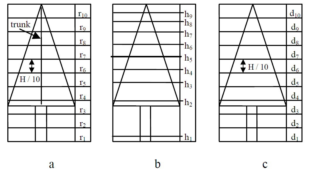
Small-footprint, high-resolution LiDAR data (25 points m-2) were used by Reitberger et al. ([26]) for detecting two tree groups (deciduous and coniferous) according to leaf-on and leaf-off conditions using an unsupervised classification of metrics extracted from LiDAR data; results for leaf-on and leaf-off conditions were 85% and 96% accurate, respectively. The unsupervised classification process used features computed from three-dimensional coordinates and pulse-intensity-width data. The following groups of metrics, or “saliencies” as they were called in Reitberger et al.’s text, were considered in the classification procedure: outer tree geometry Sg, inner tree geometry Si and intensity-related tree structure SI. Sg consists of two metrics, Sg 1 and Sg 2; both metrics select crown points from among all tree points by detecting the crown base by dividing points in a tree segment into 0.5-m vertical layers and finding the layer that contains more than 1% of the total tree points. Sg 1 contains two parameters {a,b} of a parabolic surface fitted to points found by fitting a convex hull to all points belonging to the crown. Sg 2 is the mean radius (mean distance of all points from the stem position, which in turn is estimated to be at the coordinate of the highest crown point) for each vertical layer (Fig. 2a). The Si metrics are divided into two sub-groups, Si h and Si d , which are both inspired by the tree characterization metrics developed by Naesset ([21]). Si h is the percentile of the point height distribution in a tree segment (Fig. 2b), and Si d is the percentage of total tree points in each layer (Fig. 2c). The SI metric relates to two aspects of the peak intensities detected in the waveform: SI 1 is the mean intensity in each vertical layer, and SI 2 is the overall mean intensity of all the tree points.
Fig. 2 - Tree layers for tree structuremetrics (from [25]).
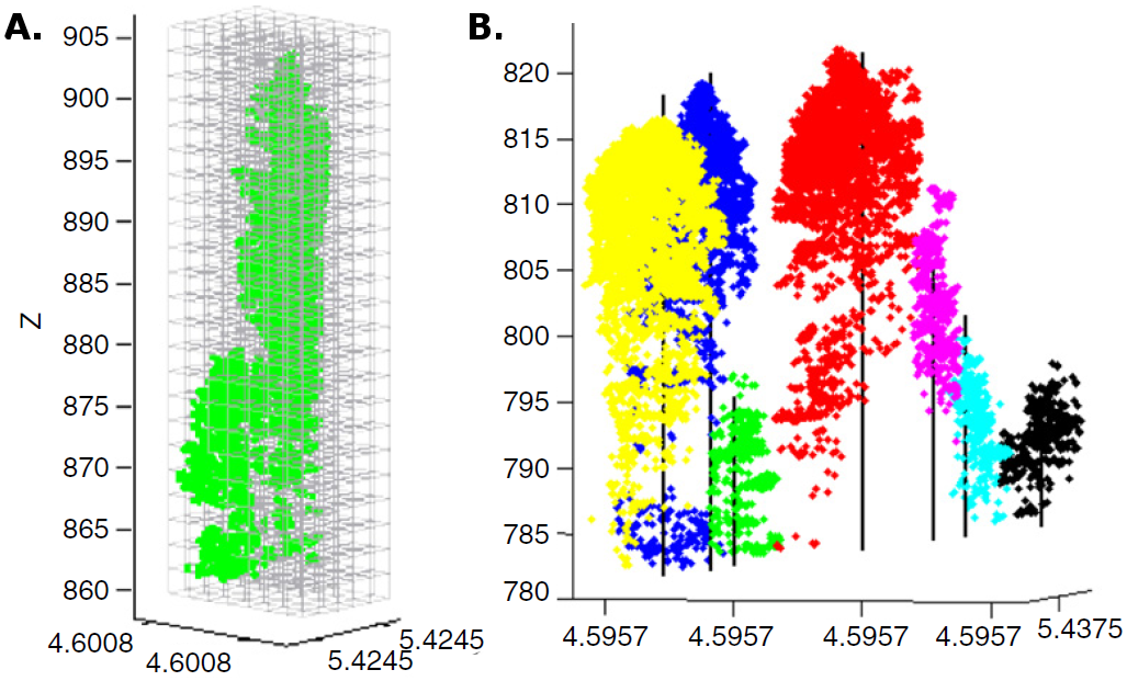
The estimation of tree positions can also be improved by stem detection using a cluster algorithm followed by stem reconstruction using a RANSAC-based adjustment ([25]). Depending on the tree density and leaf-on/leaf-off conditions, the best detection rate using this method was 61% for coniferous trees and 41% for deciduous trees. The same authors ([27]) recently developed a novel normalized cut segmentation procedure, which is based on voxel space, to detect single trees underneath the canopy (Fig. 3). When tested against a standard watershed segmentation method, the normalized cut segmentation procedure resulted in a 12% improvement and the best accuracy was 93%. It is worth noting that lowering the point density to 10 points m-2 had little effect on the accuracy of voxel-based classifications (Fig. 4).
Fig. 3 - (A): Voxel-based segmentation of dense FW LiDAR points; and (B): resulting single trees (from [28]).
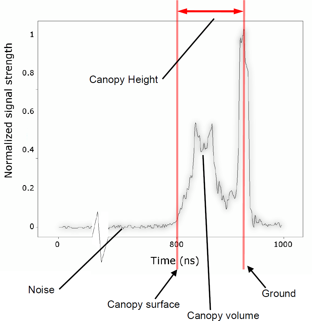
Fig. 4 - Generic waveform plot with various metrics: start of the canopy surface, canopy and ground return with the derived canopy height.
To my knowledge, the methods described above are the only tree-scale FW processing methods present in the current literature. Extensive experimentation using discrete-return LiDAR data has been performed, and therefore it is likely that future research will also produce experimental results based on FW LiDAR. Due to high point-density requirements, large acquisition costs and dataset sizes are likely to lead to longer processing times and higher overall costs, which may limit the applicability of FW LiDAR tree-scale approaches.
Small-footprint full-waveform processing for plot-scale forest structure studies
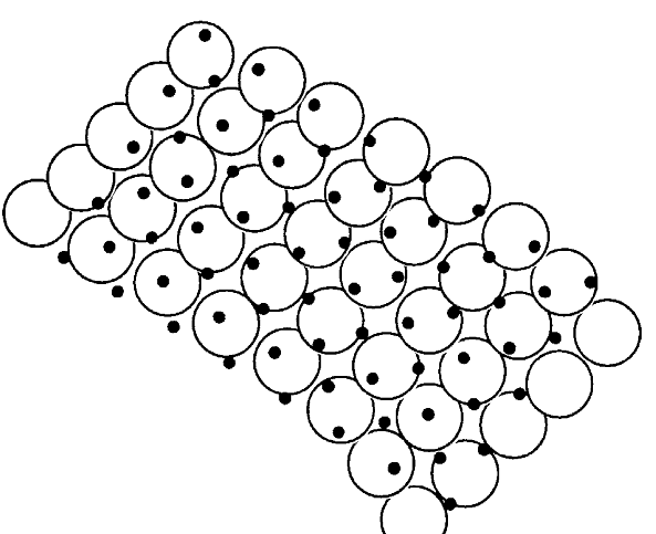
Small-footprint (<1 m) LiDAR systems use a different sampling scale than large-footprint systems; therefore, approaches to data processing differ. When using small-footprint LiDAR with a consistent point density, vegetation geometry can be modeled with greater detail because each laser pulse samples different parts of the tree; in contrast, large footprints, with a size comparable to crown diameters, sample the entire tree. Consequently, more flight time is required to cover equivalent areas when using a small footprint approach ([8]). Pulses from large-footprint sensors also reach the ground more consistently ([3]) than those from small-footprint systems because a larger area is covered by laser pulses (Fig. 5). The ability to penetrate beyond the first reflective surface of the canopy is an essential characteristic of small-footprint systems ([18]). Laser penetration is also of critical importance for calculating the height difference between ground return and canopy return ([15]), which is an essential metric for estimating tree height. Tree height is generally underestimated by 1 m ([19]) because of the probability of pulses hitting the upper-most part of the tree. The degree of height underestimation is a function of canopy type (sharp and conical canopies increase error), point density and footprint size. Height estimation bias is therefore a critical factor in the analysis of small-footprint surveys. Chauve et al. ([5]) emphasized the importance of the additional points detected by FW LiDAR, especially in the lower part of the canopy, in reducing height estimation bias and the standard deviation (5 cm).
Fig. 5 - Sampling geometry of a large-footprint LiDAR survey; circles represent laser footprints, and black dots represent a regular sampling grid (from [11]).
Wagner et al. ([30]) confirmed the importance of waveform analysis in improved vegetation mapping and classification. They applied a decision tree approach to processing LiDAR data that used the peak abundance, width and amplitude, but did not use geometric information, to create yes/no conditions for each pulse. A classification kappa accuracy coefficient of 0.8 was obtained, thus proving the accuracy of the decision tree method. Rossmann et al. ([29]) tested a large-area LiDAR survey with a 4-6 points m-2 and integrated different multispectral images (aerial and SPOT satellite sensors) to obtain an efficient forest inventory. The method of Rossmann et al. used decision tree classification criteria based on digital image analysis results for vegetation detected using a LiDAR-derived canopy height model (CHM). Tree stands with a similar stock were automatically identified and merged (when contiguous) on the map through a region-merging process. For each merged area, stand attributes were extracted using the CHM to find the dominant tree height and density, and the yield class was then derived using water balance information for the area.
Large-footprint full-waveform analysis for plot-scale forest structure studies
Drake et al. ([7]) tested metrics derived from LVIS (Laser Vegetation Imaging Sensor) data obtained over a tropical forest area. LVIS is an airborne, large-footprint FW sensor developed at NASA. In the work of Drake et al., LVIS was used with a sampling footprint size of ~25 m. The objective was to predict the field-derived quadratic mean breast height diameter (DBH), average basal area (ABA) and above-ground biomass accumulation (AGBM) at the plot and footprint levels. At the plot level, the DBH, ABA and AGBM results showed significant correlation values of up to 0.93, 0.72 and 0.93, respectively. At the footprint level, the correlation values were much lower (0.59, 0.53 and 0.27 for the DBH, ABA and AGBM, respectively). Footprint level results were weakened by the effect of a limited laser pulse positional accuracy on ground coordinates. The following metrics and relative forest parameters, derived from the return FW signal, were used:
- The location (range index) within the waveform. This metric is the point where the signal increased above a mean noise level threshold (Fig. 1) and was used to detect the canopy surface.
- The location within the waveform of the centre of the last Gaussian pulse (Fig. 1). This metric was used to detect the ground surface.
- The difference between metrics 1 and 2. This value was used to extract the canopy height.
- Height of the median energy. This metric is the location of of median energy height relative to the ground location and was used to derive the vertical arrangement of canopy elements, canopy openness and tree density.
- Median/height ratio. This metric is defined as the value derived from point 4 divided by the canopy height at point 1 and was used to estimate the median position relative to the canopy surface. Ground return ratio. This metric is the sum of all values in the last return peak divided by all other values (only values above noise level are considered) and was used to infer the degree of canopy closure.
Anderson et al. ([2]) tested the integration of LVIS data with hyperspectral data from the AVIRIS (Airborne Visible/Infrared Imaging Spectrometer) sensor to extract the quadratic mean of the DBH, ABA and AGBM over a mixed conifer-hardwood forest area. Their method included predictions of species composition and land use patterns derived from AVIRIS reflectance information in addition to above-ground biomass data estimated using LiDAR. An 8-9% improvement in correlation and a 5-8% decrease in error were found.
Harding et al. ([11]) and Lefsky et al. ([16]) tested the use of SLICER (Scanning Lidar Imager of Canopies by Echo Recovery) sensor data for canopy height profiling (CHP). SLICER provides ~10m footprints at 5000 m flying altitudes using a near-infrared (NIR - 1024 nm) wavelength laser. They observed that a stand-specific calibration was necessary because CHP and ground models can be biased depending on canopy surface characteristics; for example, conifers with sharp conical canopies and needles with low NIR reflectivity caused a greater bias (underestimation) than canopies from deciduous trees that have an NIR-bright and umbrella-like canopy.
Harding et al. ([11]) and Lefsky et al. ([16]) used six steps to transform a raw waveform to a CHP:
- smooth the signal (sum six consecutive bins) to decrease the background noise;
- find the background noise level by calculating the signal mean and variance beyond the last return;
- differentiate the ground and canopy returns. The last ground return is the last return that is a multiple of the background noise variance, and the peak of the ground return is the first inflection before the last ground return;
- adjust the amplitude to account for differences in reflectance;
- compute the height distribution of the canopy closure;
- apply an occlusion transformation to yield a normalized height distribution of the plant area.
This method has proven to be reproducible and significantly (P < 0.0001) correlated to ground-measured and LiDAR-estimated CHP for young (R2 = 0.75), intermediate (R2 = 0.52), mature (R2 = 0.33) and old-growth (R2=0.43) stands.
Lefsky et al. ([16], [17]) used SLICER data to investigate forests of different compositions, with the objective of deriving general equations for different biomes. In some cases, very high correlations of LiDAR metrics with LAI and AGBM were obtained. The first experiment found consistent correlations (up to R2 = 0.84) using a unified equation (AGBM = 0.378 · MCH2) when estimating AGBMs of temperate deciduous broadleaf, temperate coniferous needleleaf and boreal coniferous needleleaf biomes. The second study tested the ability to estimate LAI information based on SLICER data for five different temperate coniferous needleleaf biome sites containing one or more of the following species: open-canopy Pinus ponderosa, Picea sitchensis (sitka spruce), Tsuga heterophylla (western hemlock) and Abies (true fir) forests. Several indices were extracted from LiDAR metrics to derive equations for estimating tree stand structure variables. The highest correlations for all sites were 0.81 for LAI and 0.92 for AGBM. Based on these tests on different sites and conditions, it can be concluded that some equations that relate LiDAR metrics to forest parameters are valid at the regional scale.
SLICER sensor data were also used to assess vertical canopy material distributions and canopy cover. Vertical canopy distributions are essential to estimating other parameters, such as AGBM, state of the forest and age of a plantation ([15]). Canopy cover can be directly assessed by the ratio of the signal reflected by the canopy to the signal reflected by the ground ([20]). Both Lefsky et al. ([15]) and Means et al. ([20]) found a significant correlation between SLICER metrics and plot-scale average basal area.
Parker et al. ([23]) used SLICER data to extract the vertical distribution of light attenuation through a canopy, and they found a significant correlation with field measurements. Light transmittance data was obtained by Koetz et al. ([14]) by inverting a radiative transfer model (RTM), derived from a modelled FW signal, to obtain horizontal and vertical forest structure (fractional cover, LAI, maximum tree height and vertical crown expansion).
Conclusions
Full-waveform LiDAR processing is a promising technique for various forestry applications. There are important factors to consider when processing return signals. One is pulse geolocation, which must have an acceptable accuracy relative to the target spatial scale and is especially important for single-tree metrics. Another parameter that differentiates FW LiDAR surveys from other methods is the footprint size. Large footprints sample large areas; therefore, elements inside an area are mixed within the resulting return pulse shape. Because of the laser beam size, FW LiDAR has a high degree of probability of finding openings in the canopy, reaching the ground and providing a ground return signal ([16]), which is crucial for calculating an accurate CHM. In contrast, small footprints provide a “cleaner” response, and the ratio of ground to canopy returns depends on leaf density and the LiDAR point density.
It is apparent from the literature that there are numerous methods for processing FW LiDAR data for the estimation of forest parameters. Certain models are applicable at either the plot or regional level, and some methods are influenced by leaf-off/leaf-off conditions. The application context is therefore important and must be assessed before planning a LiDAR survey. It is crucial to delineate the scope of suitability for each methodology; when estimating key characteristics, such as tree height distribution, crown diameter and relative structural tree parameters, metrics derived from FW signals are not always significantly correlated. For some forest types, the correlation is very high ([1]); however, the equations are valid only when applied to specific forest types and environments ([12]).
Currently, the main drawback of performing LiDAR-based estimations is the high cost of data acquisition, especially for high-density and small-footprint surveys. Robust and dedicated software for signal processing is limited to a few proprietary products, and it is expected that future research will result in the development of dedicated open-source tools. It is reasonable to expect that FW LiDAR data processing will be used in forestry research with the same regularity as digital image analysis.
Acknowledgements
The author wishes to thank Josef Reitberger (Munich University of Applied Science) for his help on commenting part of the text. This work is part of a project financially supported by the University of Padova (Progetto di Ricerca di Ateneo 2009 - CPDA097420).
List of abbreviations
The following abbreviations have been used in this paper:
- FW: full waveform;
- AGBM: above-ground biomass;
- CHM: canopy height model;
- CHP: canopy height profile;
- MCH: mean canopy height;
- ABA: average basal area;
- DBH: breast height diameter;
- LAI: leaf area index.
Correlation values are expressed throughout the paper as the coefficient of determination, R2.
References
Gscholar
Gscholar
Gscholar
Gscholar
Gscholar
Gscholar
Gscholar
CrossRef | Gscholar
Authors’ Info
Authors’ Affiliation
Department of Land and Agroforest Environments, University of Padova - Agripolis, v.le dell’Università 16, I-35020 Legnaro (PD - Italy)
Corresponding author
Paper Info
Citation
Pirotti F (2011). Analysis of full-waveform LiDAR data for forestry applications: a review of investigations and methods. iForest 4: 100-106. - doi: 10.3832/ifor0562-004
Paper history
Received: Aug 02, 2010
Accepted: Feb 21, 2011
First online: Jun 01, 2011
Publication Date: Jun 01, 2011
Publication Time: 3.33 months
Copyright Information
© SISEF - The Italian Society of Silviculture and Forest Ecology 2011
Open Access
This article is distributed under the terms of the Creative Commons Attribution-Non Commercial 4.0 International (https://creativecommons.org/licenses/by-nc/4.0/), which permits unrestricted use, distribution, and reproduction in any medium, provided you give appropriate credit to the original author(s) and the source, provide a link to the Creative Commons license, and indicate if changes were made.
Web Metrics
Breakdown by View Type
Article Usage
Total Article Views: 106548
(from publication date up to now)
Breakdown by View Type
HTML Page Views: 89337
Abstract Page Views: 5835
PDF Downloads: 9391
Citation/Reference Downloads: 136
XML Downloads: 1849
Web Metrics
Days since publication: 5407
Overall contacts: 106548
Avg. contacts per week: 137.94
Article Citations
Article citations are based on data periodically collected from the Clarivate Web of Science web site
(last update: Mar 2025)
Total number of cites (since 2011): 74
Average cites per year: 4.93
Publication Metrics
by Dimensions ©
Articles citing this article
List of the papers citing this article based on CrossRef Cited-by.
Related Contents
iForest Similar Articles
Review Papers
Remote sensing-supported vegetation parameters for regional climate models: a brief review
vol. 3, pp. 98-101 (online: 15 July 2010)
Review Papers
Accuracy of determining specific parameters of the urban forest using remote sensing
vol. 12, pp. 498-510 (online: 02 December 2019)
Review Papers
Remote sensing of selective logging in tropical forests: current state and future directions
vol. 13, pp. 286-300 (online: 10 July 2020)
Technical Reports
Detecting tree water deficit by very low altitude remote sensing
vol. 10, pp. 215-219 (online: 11 February 2017)
Research Articles
Classification of xeric scrub forest species using machine learning and optical and LiDAR drone data capture
vol. 18, pp. 357-365 (online: 07 December 2025)
Research Articles
Assessing water quality by remote sensing in small lakes: the case study of Monticchio lakes in southern Italy
vol. 2, pp. 154-161 (online: 30 July 2009)
Research Articles
Identification and characterization of gaps and roads in the Amazon rainforest with LiDAR data
vol. 17, pp. 229-235 (online: 03 August 2024)
Research Articles
Mapping the vegetation and spatial dynamics of Sinharaja tropical rain forest incorporating NASA’s GEDI spaceborne LiDAR data and multispectral satellite images
vol. 18, pp. 45-53 (online: 01 April 2025)
Technical Reports
Remote sensing of american maple in alluvial forests: a case study in an island complex of the Loire valley (France)
vol. 13, pp. 409-416 (online: 16 September 2020)
Research Articles
Afforestation monitoring through automatic analysis of 36-years Landsat Best Available Composites
vol. 15, pp. 220-228 (online: 12 July 2022)
iForest Database Search
Search By Author
Search By Keyword
Google Scholar Search
Citing Articles
Search By Author
Search By Keywords
PubMed Search
Search By Author
Search By Keyword

