A LiDAR-based approach for a multi-purpose characterization of Alpine forests: an Italian case study
iForest - Biogeosciences and Forestry, Volume 6, Issue 3, Pages 156-168 (2013)
doi: https://doi.org/10.3832/ifor0876-006
Published: Apr 08, 2013 - Copyright © 2013 SISEF
Research Articles
Abstract
Several studies have verified the suitability of LiDAR for the estimation of forest metrics over large areas. In the present study we used LiDAR as support for the characterization of structure, volume, biomass and naturalistic value in mixed-coniferous forests of the Alpine region. Stem density, height and structure in the test plots were derived using a mathematical morphology function applied directly on the LiDAR point cloud. From these data, digital maps describing the horizontal and vertical forest structure were derived. Volume and biomass were then computed using regression models. A strong agreement (accuracy of the map = 97%, Kappa Cohen = 94%) between LiDAR land cover map (i.e., bare soil, forest, shrubs) and ground data was found, while a moderate agreement between coniferous/broadleaf map derived from LiDAR data and ground surveys was detected (accuracy = 73%, Kappa Cohen = 60%). An analysis of the forest structure map derived from LiDAR data revealed a prevalence of even-age stands (66%) in comparison to the multilayered and uneven-aged forests (20%). In particular, the even-age stands, whether adult or mature, were overwhelming (33%). A moderate agreement was then detected between this map and ground data (accuracy = 68%, Kappa Cohen = 58%). Moreover, strong correlations between LiDAR-estimated and ground-measured volume and aboveground carbon stocks were detected. Related observations also showed that stem density can be rightly estimated for adult and mature forests, but not for younger categories, because of the low LiDAR posting density (2.8 points m-2). Regarding environmental issues, this study allowed us to discriminate the different contribution of LiDAR-derived forest structure to biodiversity and ecological stability. In fact, a significant difference in floristic diversity indexes (species richness - R, Shannon index - H’) was found among structural classes, particularly between pole wood (R=15 and H’=2.8; P <0.01) and multilayer forest (R=31 and H’=3.4) or thicket (R=28 and H’=3.4) where both indexes reached their maximum values.
Keywords
Lorey’s Mean Height, Tree Volume, Carbon Stocks, Biodiversity, Species Richness, LiDAR
Introduction
In the last decade, applied environmental sciences have undergone a radical change with the emergence of new technologies related to the retrieval and processing of spatial data. In particular, modern remote sensing techniques, such as Light Detection and Ranging (LiDAR), have been playing an increasingly important role in forest description, from local (e.g., [44]) to regional ([49], [67]) or global scale ([71]), in terms of tree composition ([64]), forest structure ([18], [53], [27]), vegetation mapping ([78], [80]) and stand development ([12]). The increased market demand for wood products, and especially for wood-based bio-energy, has been requiring detailed spatial information on wood volume for forest resource planning ([76]) and biomass exploitation ([73]). Traditionally, the acquisition of these data is time consuming and expensive as they are usually obtained through field surveys. Several studies have verified the suitability of LiDAR for deriving forest metrics in large areas ([40], [26], [4], [79]). In this context, tree heights are derived from LiDAR point cloud ([50]) and then used to estimate stem volume ([72]) or aboveground biomass. Moreover, there is also a growing need for detailed spatial information to improve forest management with regard to biodiversity and carbon sequestration. In recent decades, several studies and exercises have been carried out to integrate biodiversity issues with forest inventories ([19]), but the debate on the potential role of forest inventories in biodiversity monitoring is still open ([20]). As stand structure plays a key role in deriving biodiversity indicators, LiDAR may be a useful tool in biodiversity management. For example, it appears a quite interesting tool for biodiversity related analysis, such as habitat type classification ([82], [15], [7]) and species diversity modeling ([30], [82]). Concerning with carbon sequestration, forests can sequester and store more carbon than all other terrestrial ecosystems ([35]) and exchange 90% of total carbon flow between the atmosphere and biosphere ([84]). Thus, the integration of data from inventories with remote sensing techniques is crucial for an accurate quantification of carbon stocks in forest ecosystems and to monitor the influence of human activities (i.e., forest management, afforestation, deforestation) on these stocks ([37], [29], [9], [67]).
LiDAR surveys the three-dimensional (3-D) structure of forests by measuring time-of-flight of laser pulses reflected from the target. Position and orientation of the scanning device is supplied by the Global Positioning System (GPS) and the Inertial Navigation System (INS - [42]). While filtering operations may be considered a well-established procedure ([4]), methods for extracting forest and environmental characteristics from the laser point cloud need, especially in forests with a complex structure, a robust testing and verification phase with ground-truth measurements. Although methods for the extraction of structural and dendrometric characteristics of conifer and broadleaf mature forests are already available (i.e., [5], [1]), a precise stand characterization can be more problematic in the case of young or uneven-aged multilayered mixed forests because of their intrinsic greater complexity ([21]).
Within this framework, the aims of the present study were: (i) to create and validate digital map of the horizontal and vertical forest structure derived from LiDAR data, (ii) to quantify forest volume and aboveground carbon stocks for each structural class, (iii) to verify LiDAR structural map applicability for forest vegetation characterization (i.e., species diversity and composition) in order to detect forests stands with an high naturalistic value.
Materials and methods
Materials
Study area
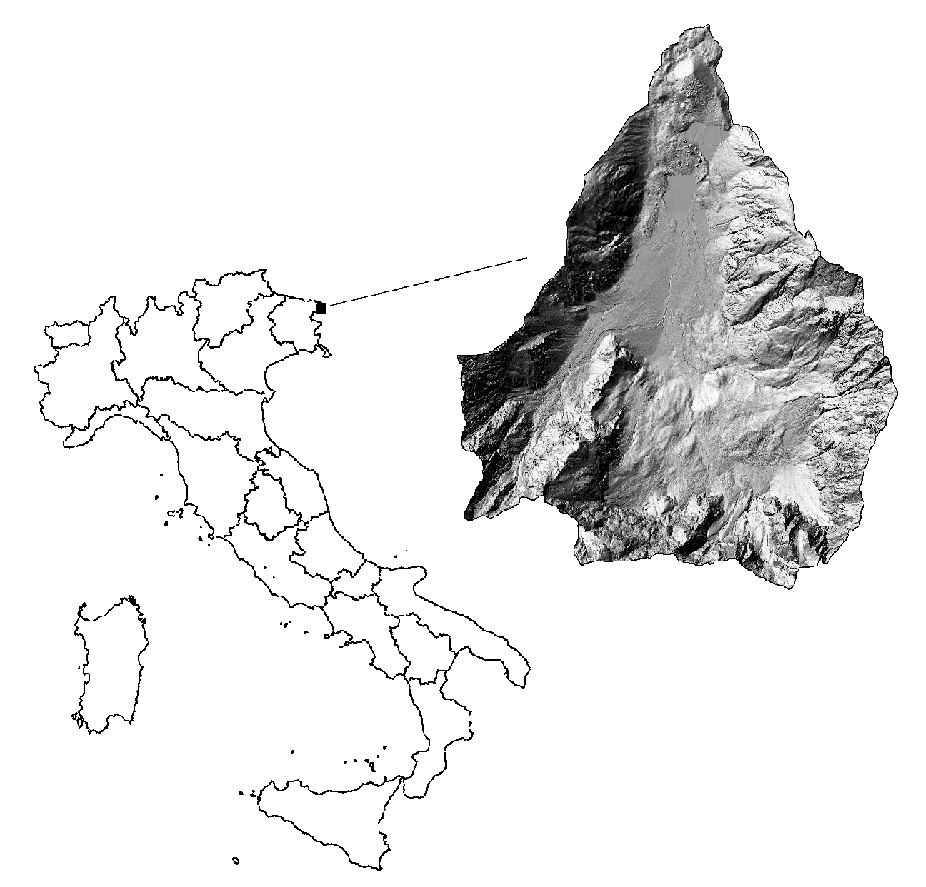
The study area is located at Fusine lakes (1 688 ha, 46°30’15” N, 13°38’26” E - Fig. 1), in north-eastern Alps near the Italian border with Slovenia and Austria. The site is characterized by patches of pastures surrounded by spruce forests or spruce, fir and beech mixed forests (Picea abies Karst., Abies alba Mill. and Fagus sylvatica L., respectively - Tab. 1). Mean annual temperature at the Fusine lakes is 7.3° C with an absolute maximum of 28° C and an absolute minimum of -27° C. The area is characterized by a strong annual and daily temperature range (22° C). Annual rainfall is 1520 mm. Bedrock is mainly dolomite. The study area includes 13 forest compartments belonging to the Regional Government for an area of 665 ha: 7 compartments are forests managed for wood production, 4 are left to natural evolution, 1 compartment has a recreational destination and 1 is unproductive.
Fig. 1 - Study area.
Tab. 1 - Land covers in the study area derived from Moland Land Use map.
| Land use | Area (ha) |
% |
|---|---|---|
| Mixed forests | 631 | 37.4 |
| Bare rocks | 471 | 27.9 |
| Heath and scrubs | 261 | 15.5 |
| Coniferous forests | 208 | 12.4 |
| Pastures and grasslands | 77 | 4.6 |
| Water bodies | 23 | 1.4 |
| Hardwood forests | 12 | 0.7 |
| Scrublands | 3 | 0.2 |
| Total | 1 688 | - |
LiDAR and ground data acquisition
LiDAR data were acquired in October 2006 (85% of the study area) and in July 2009 (15% of the study area) using an Optech ALTM 3100 sensor onboard a helicopter. Average pulse density was 2.8 points per square meter. The flight height was about 1000 m above ground level, the maximum scan angle was ± 18° and a beam divergence was 0.2 mrad (~20 cm at 1000 m distance). Data were collected on a multi-pulse mode with a maximum of four return echoes registered for each emitted pulse.
Ground-truth points were distributed accor-ding to a stratified sampling design. A square grid with cells of 100 x 100 m was overlaid on the structural map obtained from LiDAR data (see “Methods”) and 37 of them were distributed proportionally to each structural class and then randomly selected. The survey was performed during summer 2010. Trees were surveyed within a circular plot of 13 m radius or 4 m radius depending on their diameter at breast height (DBH > 7.5 cm and DBH < 7.5 cm, respectively). In each plot, all standing trees were identified and their DBH were measured. Total height was measured on a subsample of ten trees distributed on different diameter classes.
Within each circular plot, a 100 m2 square subplot was identified for a vegetational survey according to Braun-Blanquet ([11]) and Westhoff & Van Der Maarel ([83]). In particular, the following attributes were investigated:
- the cover of each forest layer according to the following scheme: trees > 3 m high; shrubs > 0.5 m and < 3 m in height; herbaceous (all grasses, ferns, and woody species < 0.5 m in height);
- the proportional cover of each vascular censed species according to Braun-Blanquet ([11]) scale, modified by Pignatti ([55]).
Flora nomenclature followed [60], phytosociological nomenclature was defined according to studies from Marincek et al. ([45]), Poldini & Nardini ([59]) and Oberdorfer ([52]). The attribution of biological forms ([63]) followed Pignatti ([56]).
Methods
Land cover, coniferous/broadleaf and forest structure maps
In order to derive land cover, coniferous/ broadleaf and forest structure maps from raw LiDAR data, a individual tree crown approach (ITC) was used ([6]). LiDAR data processing was performed using ZEUS software (© e-Laser srl - ⇒ http://www⇒ . e-laser.it/) in order to classify ground and vegetation points through semi-automatic filtering (Axelsson 2000). A manual check and refinement for areas with complex morphology was also performed. A Digital Terrain Model (DTM) with a 1 x 1 m cell resolution was created using filtered ground data and was used to derive individual tree heights using the methods reported by Barilotti et al. ([5]). This method is based on a mathematical morphology function derived from the theory proposed by Serra ([68], [69]). The function, originally developed to extract the peak elements of a raster image, was adapted to detect spatial position (x, y, z) of each tree vertex directly on the point cloud. It was then assumed that the vertex coordinates correspond to the position of each tree.
The distinction between forested and non-forested areas (land cover map) was made by using an algorithm that automatically detects the openings of the forest cover through classification of the values obtained from the Laser Penetration Index (LPI - [4]). Classified pixels were then grouped in homogenous cover classes according to the following definitions:
- forest: land with tree crown cover (or equivalent stocking level) of more than 20% and area larger than 0.2 ha;
- shrubland: vegetation lower than 3 meters above ground;
- bare soil.
Coniferous/broadleaves map was obtained through an automated extraction of individual trees using a “Top Hat” algorithm followed by an automatic crown delineation ([5]). Points which depended on the same crown were identified through a cluster analysis and each crown was delineated using circular polygons whose center and radius were calculated according to the planimetric coordinates of points belonging to each cluster. Crown depth was calculated as the difference between maximum and minimum height of point belonging to the cluster and total tree height was determined by subtracting DTM from crown vertex. Following previous work by Barilotti et al. ([6]), trees were then classified as broadleaves or conifers according to parabolic surfaces approximating crown points’ distribution and coniferous and broadleaf trees were grouped in homogeneous polygons through a region growing algorithm ([33]). Finally, areas with a presence of conifers or broadleaves higher than 65% were treated as coniferous or broadleaf stands, respectively. Otherwise, they were treated as mixed forests.
The forest structure map was obtained through a classification of tree heights within forest areas following the criteria reported in Tab. 2. Also in this case, areas with an homogeneous distribution of tree height classes were delimited through a region growing algorithm ([33]). Main structural categories adopted in Tab. 2 followed the definitions used for forest management plans in the Region Friuli Venezia Giulia (regeneration phase, ticket, pole wood, adult forest, mature forest, multilayer forest - [58], [24]). However, as most of the forest stands in the area are managed according to shelterwood system on small areas, we also used a more detailed structural type classification (Tab. 2) in order to better underline the different forest development stages (i.e., stand after regeneration cut or stand after final cut). In order to better distinguish shrublands from regeneration phase, a manual check using the available digital areal photos for the area and considering elevation was performed.
Tab. 2 - Structural classes and structural types as defined by Del Favero et al. ([24]) and Barilotti et al. ([6]).
| Structural class | Structural type |
Height (m) |
Notes |
|---|---|---|---|
| Regeneration phase | Regeneration phase 1 | 0 < h < 3 | No trees from the higher height class are present |
| Regeneration phase 2 | Few trees from the higher height class are present | ||
| Thicket | Thicket 1 | 3 < h < 10 | No trees from the higher height class |
| Thicket 2 | Trees from the higher height class are also present | ||
| Pole wood | Pole wood 1 | 10 < h < 20 | No trees from the higher height class |
| Pole wood 2 | Trees from the higher height class are also present | ||
| Pole wood 3 | Tending to two layer forest | ||
| Adult forest | Adult forest | 18 < h < 25 | - |
| Mature forest | Mature forest | h > 25 | - |
| Multilayer forest | Two-layered forest | - | Two clear layers can be identified |
| Multilayer forest | - | - |
Ground data elaborations
Starting from measured diameters and heights, specific height curves [i.e., H = f(DBH)] were derived and Lorey’s mean height (LMH) was calculated for each plot. LMH weights the contribution of trees to the stand height by their basal area, and is more stable than an unweighted mean height, because it is less affected by mortality and harvesting of the smaller trees. Biomass and volume were calculated according the regional allometric relationships proposed by Del Favero et al. ([24]) and Anfodillo et al. ([2]) and already applied by De Simon et al. ([25]) in the Region.
Estimated Braun-Blanquet scale values were transformed in a 1-9 ordinal transform scale as proposed by Westhoff & Van Der Maarel ([83]) before statistical analysis of species cover. The characterization of the vegetation was performed through a Canonical (Constrained) Correspondence Analysis (CCA - [74], [41], [85]) based on the relevés matrix and environmental factors matrix (i.e., LiDAR structures), and a cluster analysis, applied to plot vegetation relevés, using a similarity ratio algorithm ([83]) and Ward’s aggregation method. The statistical significance of CCA was assessed by Monte Carlo permutation tests, using 500 permutations ([75]).
Biodiversity was quantified within each plot with specific indexes such as the floristic richness (number of species surveyed for sample area) and the Shannon diversity index ([70]).
The biological spectrum percentage values were transformed with an arcsin angular transformation before the application of the analysis of variance ([38]). Normality of the compared groups (i.e., biodiversity, biological spectrum group of each LiDAR structure category) was verified using the Shapiro’s test for normality (Shapiro test, p>0.05), while the homogeneity of variances was tested using the Bartlett’s test (p>0.05). Averages for each structural category were finally compared through an ANOVA (p<0.05) with post-hoc tests (Tukey test), for biodiversity indexes, and Kruskal-Wallis ANOVA by ranks (p<0.05) with non-parametric post-hoc tests (Nemenyi-Damico-Wolfe-Dunn test), for biological forms groups. All the statistical analyses were performed using R (© R-Development Core Team).
LiDAR data validation
The validation of LiDAR structural data was performed following two methodologies depending on data type: for quality attributes (land cover map; coniferous/broadleaf map; forest structure map), Cohen’s kappa coefficient ([14]) was used, while for quantitative attributes (i.e., height, stand density, biomass) linear and non-linear regressions or analysis of variance (ANOVA) in SigmaPlot 11 (Systat® Software Inc.) were used.
Kappa coefficient can be used as a measure of agreement between model predictions and reality ([16]) or to determine if the values contained in an error matrix represent a result significantly better than random ([36]). In particular, contingency tables based on ground points were built: columns were reference data, rows were LiDAR classifications. In the case of land cover map validation, a contingency table based on all 100 x 100 m grid points within the study area was built (1694 points) and real land cover was assessed through visual photo-interpretation at each sampling point using a 2007 digital aerial photos available for the study area. Coniferous/ broadleaf map and forest structure map were both validated using the 37 ground points for which dendrometric measurements were available.
Kappa coefficient (κ) was computed according to the following equation (eqn. 1):
where Pr(a) is the relative observed agreement among raters, and Pr(e) is the hypothetical probability of chance agreement, using the observed data to calculate the probabilities of each observer randomly saying each category. If the raters are in complete agreement then κ = 1. If there is no agreement among the raters other than what would be expected by chance - as defined by Pr(e) -, κ = 0.
Results
Land cover and coniferous/broadleaf map validation
The contingency table used to validate the land cover map is reported in Tab. 3. Based on criteria established by Landis & Koch ([39]), a strong agreement between the map and ground data was found: the accuracy of the map was 97% (1638 were rightly classified) and K-Cohen was equal to 94%. Instead, a moderate agreement between coniferous/broadleaf map and ground data (data not shown) was found: map accuracy was 73% and K-Cohen was equal to 60%. The comparison between map and ground data did not improve if only trees larger than 12.5 cm were considered in the analysis (accuracy = 70%, K-Cohen = 58%).
Tab. 3 - Contingency table and calculation of Kappa Cohen’s coefficient for the validation of cover use map.
| LIDAR map | Field plots | |||
|---|---|---|---|---|
| bare soil | forest | shrubs | Samples | |
| bare soil | 603 | 5 | 23 | 631 |
| forest | 2 | 917 | 9 | 928 |
| shrubs | 12 | 5 | 118 | 135 |
| Samples | 617 | 927 | 150 | 1694 |
| Sample size | 1694 | - | - | - |
| Correctly classified | 1638 | - | - | - |
| Accuracy | 97% | - | - | - |
| P chance | 47% | - | - | - |
| K-Cohen | 94% | - | - | - |
Forest structure map validation
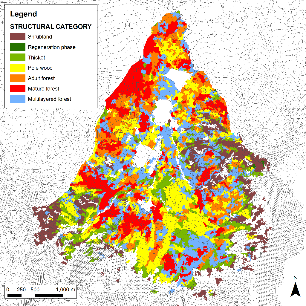
The analysis of the forest structure map derived from LiDAR data revealed a prevalence of even-age stands (66%) in comparison to the multilayered and uneven-aged forests (20% - Fig. 2, Tab. 2). In particular, the even-age stands, whether adult or mature, were overwhelming (33%). However, if we consider the structural categories separately, the most represented in terms of hectares was the pole wood (21%), while the regeneration phase was less present (<1%). The lack of this last category is partly due to the difficulties in separating it from scrublands or from two-layered stands because of the particular forest management applied in the study area (shelterwood system on small areas). In such a system, the seed cut often results in two-layered structures with plants of the previous cycle in the upper layer and a dense regeneration in the understory. Although the category “two-layered forest” is poorly represented (2%), this situation is better highlighted if the structural types are considered separately instead of aggregating them. In fact, there is a significant presence of “pole wood 2” and “pole wood 3” types which are stands with the presence of plants of the old cycle even if the regeneration is quite widespread (Tab. 4). In order to get an easier comparison between LiDAR and ground data, it was decided to show most of the results at category level and fall to type only in few cases for a more detailed analysis.
Fig. 2 - Forest structure map.
Tab. 4 - Area covered by each forest category and forest type identified from LiDAR data.
| Category | Type | Area (ha) |
Category (% of total area) |
Type (% of total area) |
|---|---|---|---|---|
| Scrubland | Scrubland | 127.9 | 12 | 12 |
| Regeneration phase | Regeneration 1 | 0 | 0 | 0.2 |
| Regeneration 2 | 1.8 | 0.2 | ||
| Thicket | Thicket 1 | 45.4 | 4 | 11 |
| Thicket 2 | 74.7 | 7 | ||
| Pole wood | Pole wood 1 | 60.1 | 6 | 21 |
| Pole wood 2 | 152.5 | 14 | ||
| Pole wood 3 | 10.6 | 1 | ||
| Adult forest | Adult forest | 168.9 | 16 | 16 |
| Mature forest | Mature forest | 180.3 | 17 | 17 |
| Multilayer forest | Two-layered forest | 22.8 | 2 | 2 |
| Multilayer forest | 207.3 | 20 | 20 | |
| Total | - | 1052.3 | - | - |
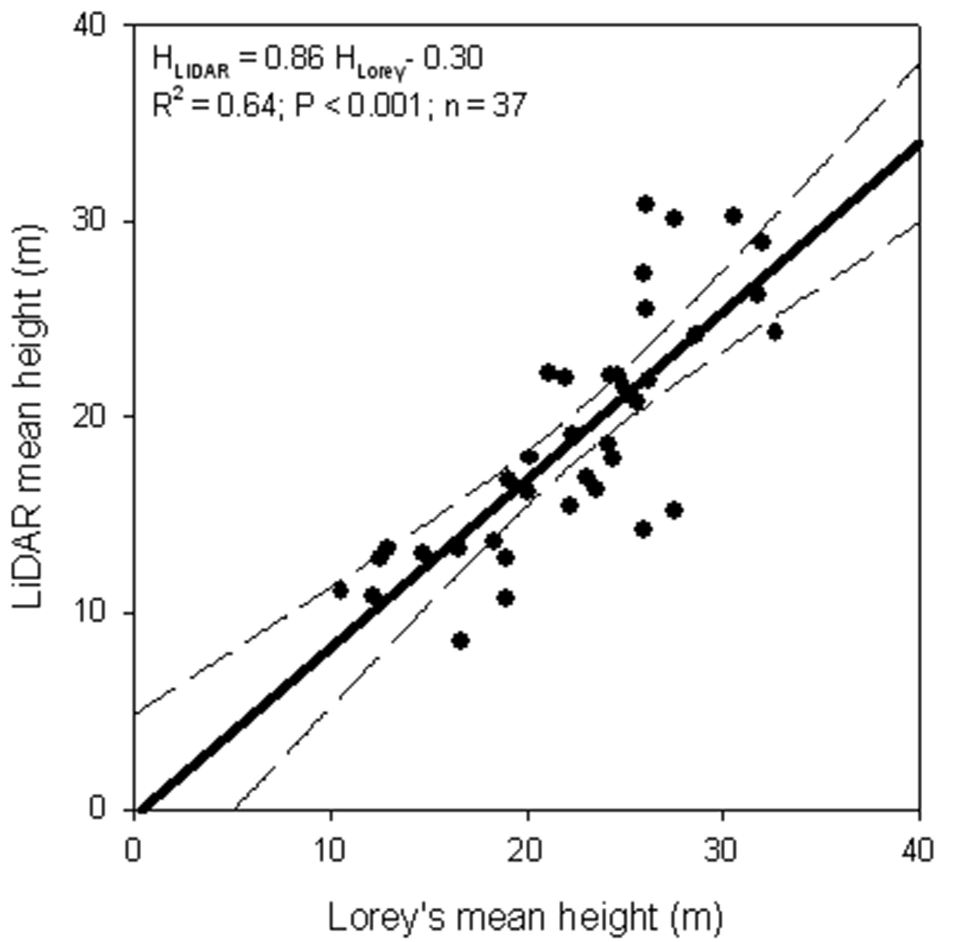
Mean stand characteristics for each forest category, as derived from ground plots, are reported in Tab. 5. Comparing LiDAR forest structure map with ground surveys, a highly significant correlation between average height derived from LiDAR and Lorey’s mean height was detected (HLiDAR = 0.86 x HLorey - 0.30; R2 = 0.64; P <0.001; trees with DBH > 4.5 cm - Fig. 3). The underestimation of mean height using LiDAR is probably due to difficulties in detecting small diameter trees because of the low posting density. This density was probably enough in the case of adult or mature forests, but it was insufficient for thicket or pole wood where stem density could be more than 2000 trees ha-1. In fact, if only trees with a DBH greater than 12.5 cm were considered, there was a strong agreement between LiDAR-estimated mean height and Lorey’s mean height (HLiDAR = HLorey - 5.35; intercepts not significantly different from zero; R2 = 0.57; P< 0.001).
Tab. 5 - Characteristics of the main forest categories derived from ground plots (mean ± standard error). (Hlorey): Lorey’s mean height; (Hd): dominant height (mean height of the dominant trees in an even-aged stands); (S): top height (mean height of the trees with the largest DBH in a stand uneven-aged stands).
| Category | Stand density (n ha-1) |
Basal area (m2 ha-1) |
HLorey (m) |
Hd or S (m) |
||
|---|---|---|---|---|---|---|
| total | d> 12.5 cm | total | d> 12.5 cm | |||
| Thicket | 2746 ± 1761 | 386 ± 9 | 23.0 ± 4.4 | 12.8 ± 1.8 | 15.5 ± 3.4 | 22.3 ± 1.3 |
| Pole wood | 2246 ± 286 | 689 ± 91 | 36.4 ± 3.7 | 27.8 ± 4.8 | 18.4 ± 1.3 | 24.2 ± 1.2 |
| Adult forest | 691 ± 101 | 656 ± 93 | 45.3 ± 5.2 | 45.1 ± 5.2 | 24.6 ± 0.7 | 28.5 ± 0.8 |
| Mature forest | 537 ± 88 | 471 ± 69 | 63.9 ± 5.1 | 63.4 ± 5.3 | 30.7 ± 1.1 | 34.3 ± 0.9 |
| Multilayer forest | 1014 ± 169 | 569 ± 86 | 43.0 ± 5.1 | 40.4 ± 4.9 | 25.1 ± 1.1 | 34.2 ± 1.2 |
Fig. 3 - LiDAR-estimated mean height vs. Lorey’s mean height (all trees with DBH greater than 4.5 cm). The continuous line indicates the regression line. The intercept is not significantly different from zero (P = 0.90). The dashed lines indicate 95% confidence intervals.
The correlation between stem density estimated from LiDAR data and measured in the field was not significant when considering all categories (data not shown), whereas correlation considering adult and mature forest (DBH greater than 12.5 cm) was significant (DLiDAR = 0.31 x Dplot + 174; R2 = 0.71; P <0.01) although the LiDAR tended to underestimate the density.
The overall accuracy of the LiDAR forest structure map was 68% (25 of 32 ground points matched with those reported from the map). Thus, a moderate agreement was detected between the map and ground data (Kappa Cohen coefficient was equal to 58% - [39]). The major discrepancies were found especially for pole woods and multilayered stands, while the greatest agreement was found for adult and mature forests. Again, this can be attributed to the high tree density in the young phases (pole wood and thicket) and to the low LiDAR posting density.
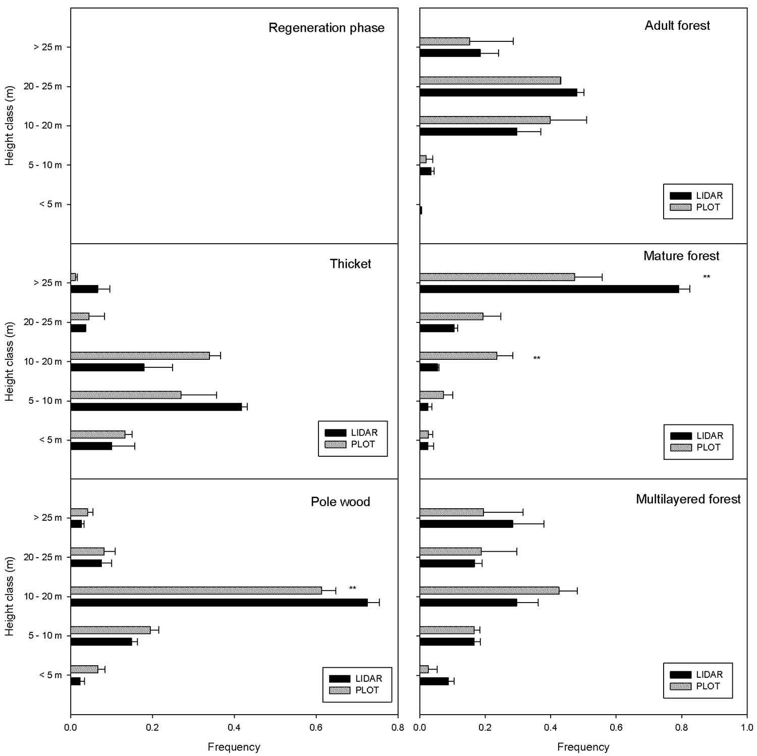
If only the 25 points for which there was a perfect correspondence between the ground and LiDAR are considered (Fig. 4), it is possible to describe the vertical distribution of the trees within the canopy. In the thicket, most of the trees were below 10 m and no significant differences were detected between LiDAR and ground plot data for any height class (P > 0.05). In the pole wood, most of the trees were between 10-20 m and a significant difference between LiDAR and ground survey was detected only for the class 10-20 m class (P <0.001). The adult forest was mainly composed of trees higher than 20 m and no differences were detected between LiDAR and ground survey for any height class (P > 0.05). In the case of mature forest, a significant difference was detected for the class 10-20 m and for the class > 25 m (P < 0.001). In the multilayered stands there was not a dominant height class and no differences were detected between LiDAR and ground survey.
Fig. 4 - Mean stem distribution in height classes for the different structural categories. The twenty-five points for which there was a perfect correspondence between the ground and LiDAR data are reported. The category “multilayer forest” includes also “two-layer stands”. The horizontal bars indicate the standard error of the mean. Asterisks indicate a significant difference (P<0.001) between LiDAR and ground survey for a specific height class.
If the points for which there was not a match between map and ground data are considered (data not shown), the two most common differences between LiDAR and ground survey results were respectively: (1) multilayer forest instead of pole wood; (2) mature forest instead of multilayer forest. In the first case, the classification error was probably related to the impossibility for LiDAR to detect correctly the dominant plants. In the second case, the discrepancy may be related to plot size that did not allow us to detect trees of the old cycle. Moreover, this error may also be related to the fact that LiDAR data refers to 2006-2009, while the measurements were carried out in 2010-2011 and then the plants of the old cycle may have already been cut in the meantime.
Volume and aboveground carbon stocks
On average, total standing volume derived from ground plots was equal to 509 ± 37 m3 ha-1, while standing volume for trees with DBH greater than 12.5 cm was equal to 469 ± 42 m3 ha-1. Mature forest had the highest total standing volume (805 ± 83 m3 ha-1) followed by adult and multilayer forest (589 ± 63 and 521 ± 75 m3 ha-1, respectively). Thicket had the lowest standing volume (201 ± 27 m3 ha-1) followed by pole wood (419 ± 49 m3 ha-1).
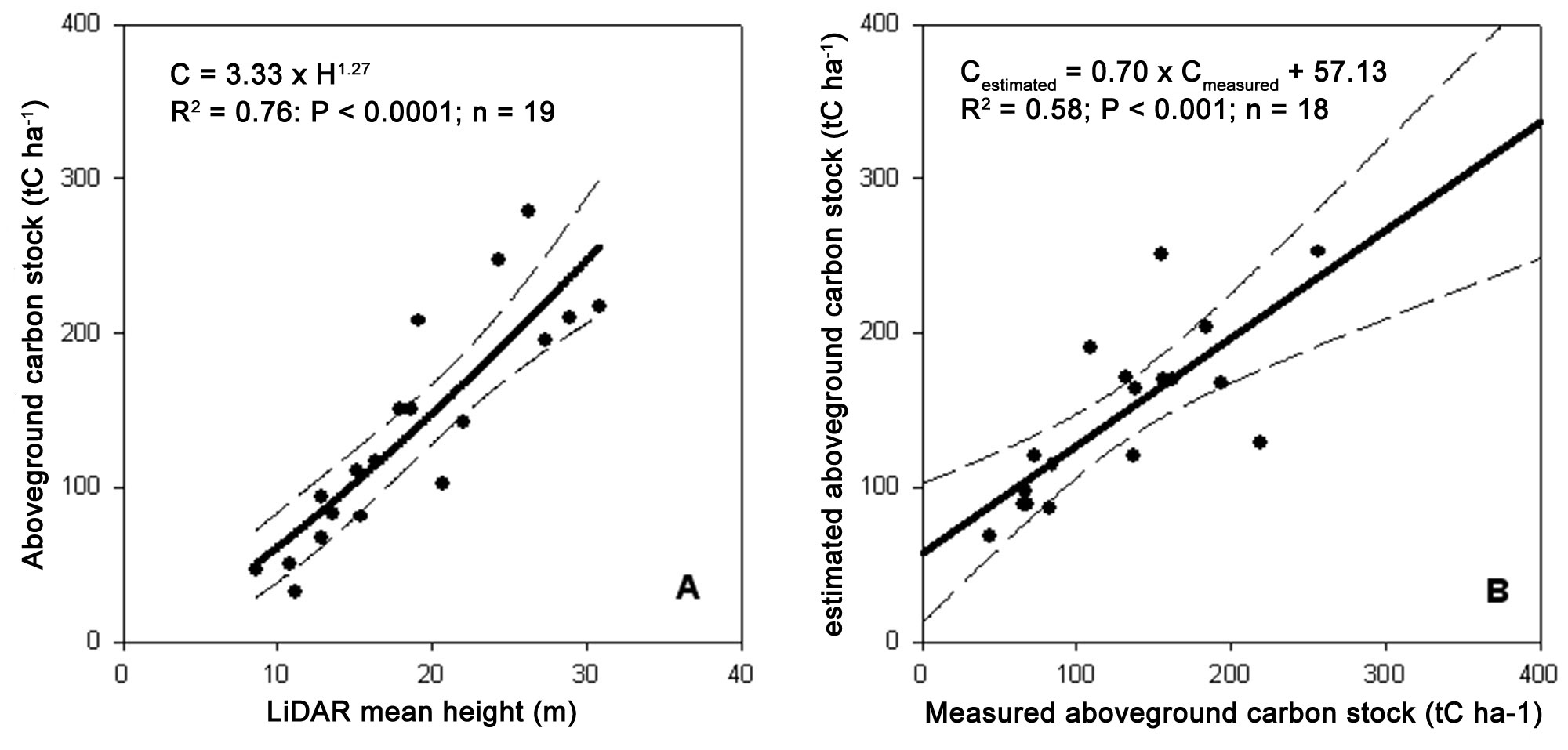
A power function was fitted on standing volume data using LiDAR-estimated mean height as independent variable. For model calibration, we randomly selected 19 ground plots. Total standing volume was significantly related to the average height derived from LiDAR data (V = 16.2 · H1.19; R2=0.80; P<0.0001 - Fig. 5a) explaining 80% of the volume variability. Model validation was performed using the remaining plots and it was also significant (R2=0.58; P <0.001 - Fig. 5b). Similar to the volume, LiDAR-estimated mean height was a good estimator of the aboveground carbon stock (C = 3.33 H1.27; R2=0.76; P<0.0001 - Fig. 6a and Fig. 6b). Overall, the carbon stock in the study area was 128.631 MgC, corresponding to 139 MgC ha-1. Most of the stock was located in adult and mature forests (27 808 and 39 116 MgC, respectively).
Fig. 5 - Model calibration to estimate total aboveground standing volume (A) and its validation (B). For calibration 19 plots were randomly selected and standing volume was plotted against LiDAR- estimated mean height. For validation, the remaining plots were used. The dashed lines represent the 95% confidence intervals.
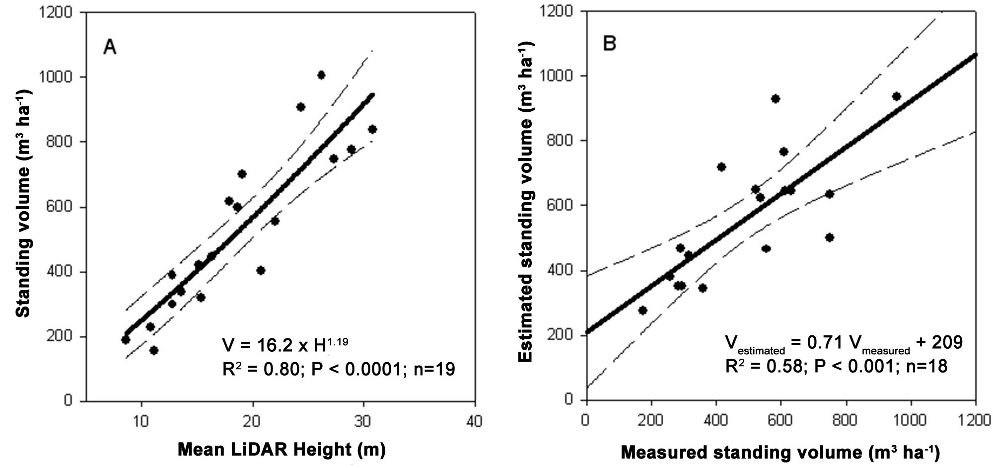
Fig. 6 - Model calibration to estimate total aboveground carbon stock (A) and its validation (B). For calibration 19 plots were randomly selected and aboveground carbon stock was plotted against LiDAR-estimated mean height. For validation, the remaining plots were used. The dashed lines represent the 95% confidence intervals.
Vegetation analysis
Biodiversity and life-form plant functional type
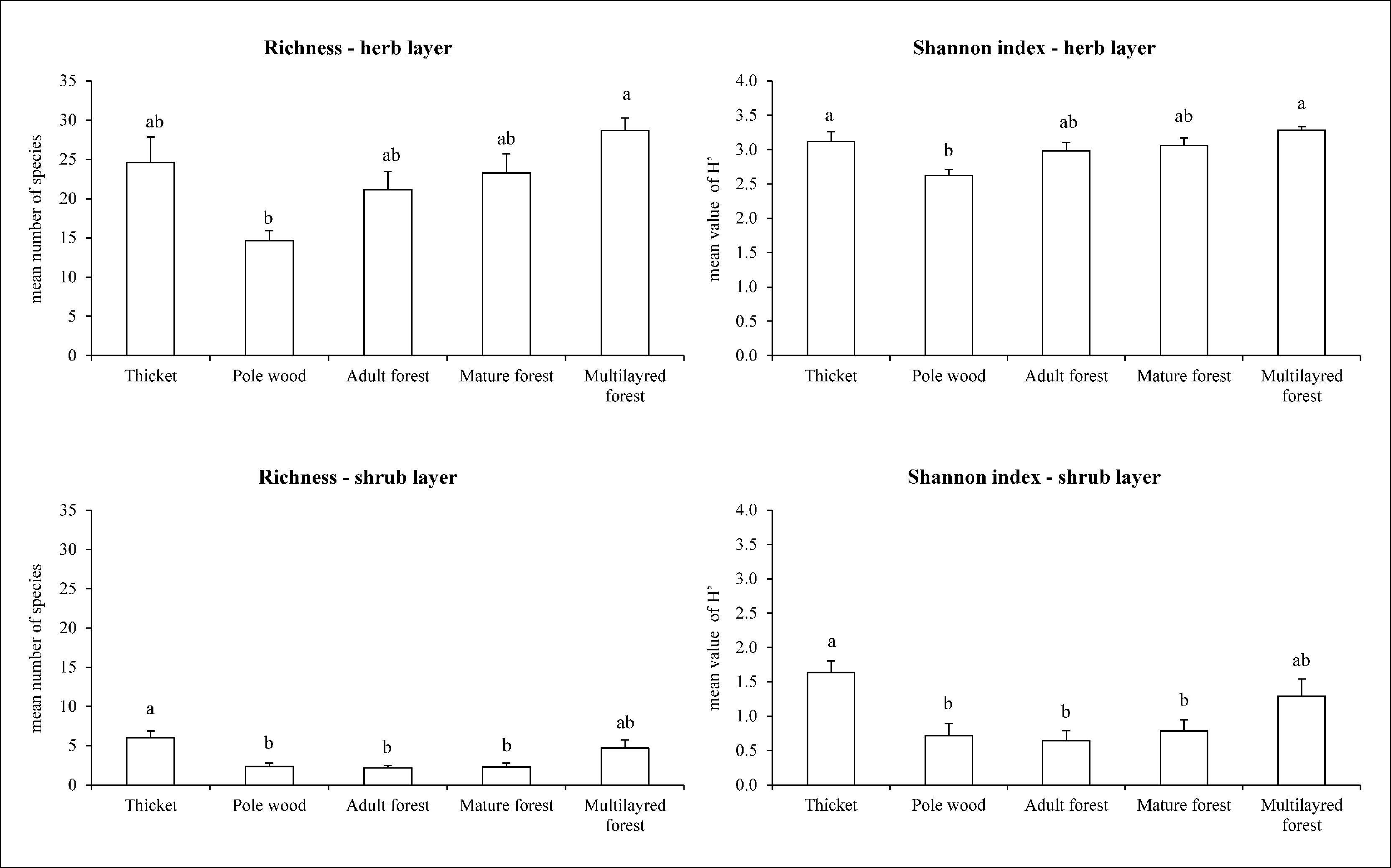
In total, 144 taxa (including species, subspecies and variety) belonging to 49 families were identified, with an average of 24 taxa for each plot. A significant difference in floristic diversity indexes (species richness - R; Shannon index - H’) was found between pole wood (R=15 and H’=2.8; P <0.01 - Fig. 7) and multilayer forest (R=31 and H’=3.4) or thicket (R=28 and H’=3.4), where both the indexes reached their maximum values. On the other hand, mature (R=25 and H’=3.2) and adult forests (R=22 and H’=3.1) did not significantly differ from the other LiDAR classes (P>0.05 - Fig. 7). Plant biodiversity was mainly related to the understory richness (Fig. 8) and in particular to the herb layer contribution which, on the average, showed 22 taxa and an H’ of 3.0. Within the herb layer, multilayer forest had the highest values for both the indexes (R=29, H’=3.3), while pole wood showed significant lower values (R=15, H’=2.6). An increase in herbaceous species number from young (pole wood) to mature stages (mature and adult forest) was also found. For shrub layer diversity, significant differences between thicket and pole wood, mature and adult forest were found (Fig. 8).
Fig. 7 - Overall biodiversity indexes and LiDAR forest structural categories. Different letter indicate statistical significance (P<0.05).
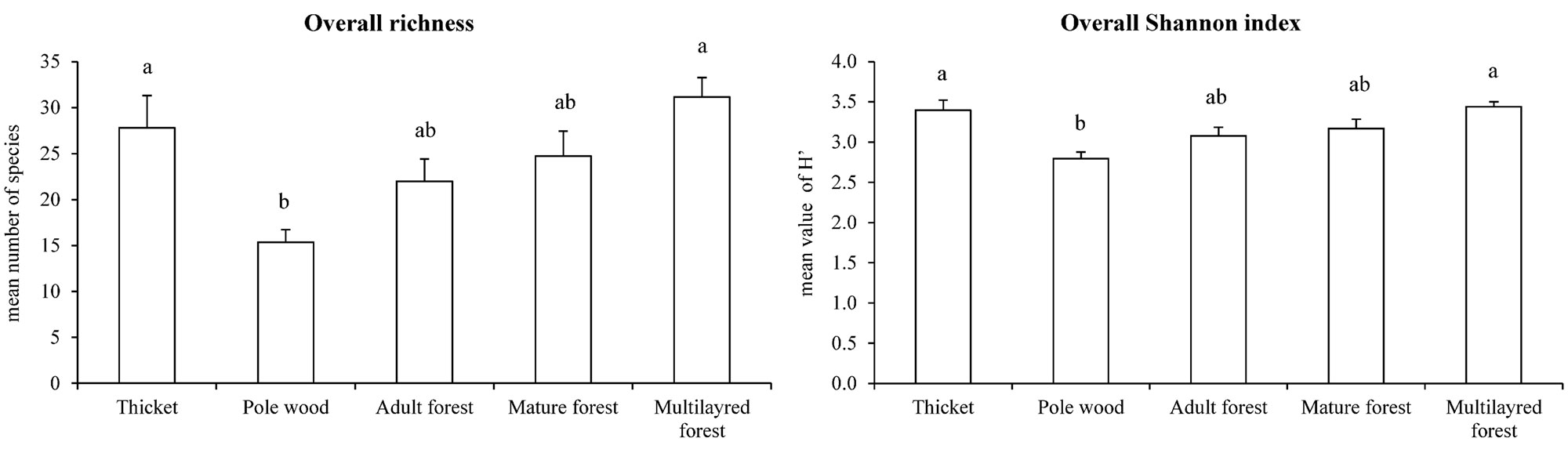
Fig. 8 - Forest layers biodiversity indexes and LiDAR forest structural categories. Different letter indicate statistical significance (P<0.05).
As expected, all forest stands were quite homogeneous in terms of tree species composition. However, the highest tree species number was found in thicket (R=3.0) and multilayer forest (R=2.2) while pole wood, adult and mature forest showed the same values (R=1.8).
In terms of biological spectrum, the hemicryptophytes (H: 55%), geophytes (G: 23 %) and phanerophytes (P: 15%) were the most represented life forms groups while chamaephytes (Ch: 6%) and therophytes (T: 1%) showed the low values.
Comparing the structural categories, only geophytes group displayed significant differences (Tab. 6). Pole wood showed the highest values, while other structural categories (mature and old forest) had intermediate ones: hemicryptophytes and chamaephytes showed higher values in thicket/multilayer stands and pole wood, respectively; phanerophytes reached the maximum value in thicket stands while therophytes were minor.
Tab. 6 - Frequencies of life forms in each LiDAR structure category. (Ch): Chamaephytes; (G): Geophytes; (H): Hemicryptophytes; (P): Phanerophytes; (NP): Nano- Phanerophytes; (T): Therophytes. Mean values and standard deviation (± SD) are showed. Different letters indicate a significant difference (P<0.05) .
| Category | Ch | G | H | P (inc. NP) | T |
|---|---|---|---|---|---|
| Thicket | 0.08 ± 0.02 | 0.28 ± 0.10 ab | 0.38 ± 0.09 | 0.26 ± 0.05 | - |
| Pole wood | 0.04 ± 0.05 | 0.41 ± 0.11 a | 0.33 ± 0.09 | 0.22 ± 0.07 | - |
| Adult forest | 0.08 ± 0.06 | 0.35 ± 0.05 a | 0.36 ± 0.11 | 0.21 ± 0.06 | 0.00 ± 0.01 |
| Mature forest | 0.07 ± 0.06 | 0.30 ± 0.09 ab | 0.44 ± 0.10 | 0.17 ± 0.04 | 0.01 ± 0.02 |
| Multilayred forest | 0.10 ± 0.06 | 0.23 ± 0.06 b | 0.47 ± 0.13 | 0.19 ± 0.07 | 0.01 ± 0.01 |
Characterization of vegetation by structure map stand
CCA showed that 13 % of the variability was explained by constrained variables (P < 0.01 - Tab. 7, Fig. 9). The remaining variability was due to the great heterogeneity of the site flora, as better described by cluster analysis. Despite of the low percentage of explained variability, it was possible to highlight two main trends. In particular, CCA1 axis identified a positive trend related to soil evolution from primitive limestone (i.e., thicket, pole wood), characterized by pioneer shrub species (e.g., Salix spp. and Corylus avellana), to medium evolved limestone soil, characterized by exigent species such as Lonicera caerulea, Dactylorhiza fuchsii and Listera cordata. CCA2 axis described a successional process of forest evolution which discriminates young and open forests (i.e., thicket and multilayer forest) and mature forests (i.e., pole wood, mature and adult stands). This trend was explained by a progressive change from pioneer and open forest species to high environmental stability and demanding mix forest species, such as Cardamine pentaphyllos, Actaea spicata and Stellaria nemorum.
Tab. 7 - CCA eigenvalues. Total inertia = 3.88, Constrained = 0.50 (13%, P>0.01).
| Parameters | CCA1 | CCA2 | CCA3 | CCA4 |
|---|---|---|---|---|
| Eigenvalues for constrained axes | 0.17 | 0.15 | 0.12 | 0.07 |
| Proportion explained | 0.34 | 0.29 | 0.24 | 0.13 |
| Cumulative proportion | 0.34 | 0.63 | 0.87 | 1.00 |
| Species-environment correlations | 0.89 | 0.82 | 0.84 | 0.81 |
Fig. 9 - CCA biplot. The numbers indicate samples sites, and the solid circles indicate plant species.
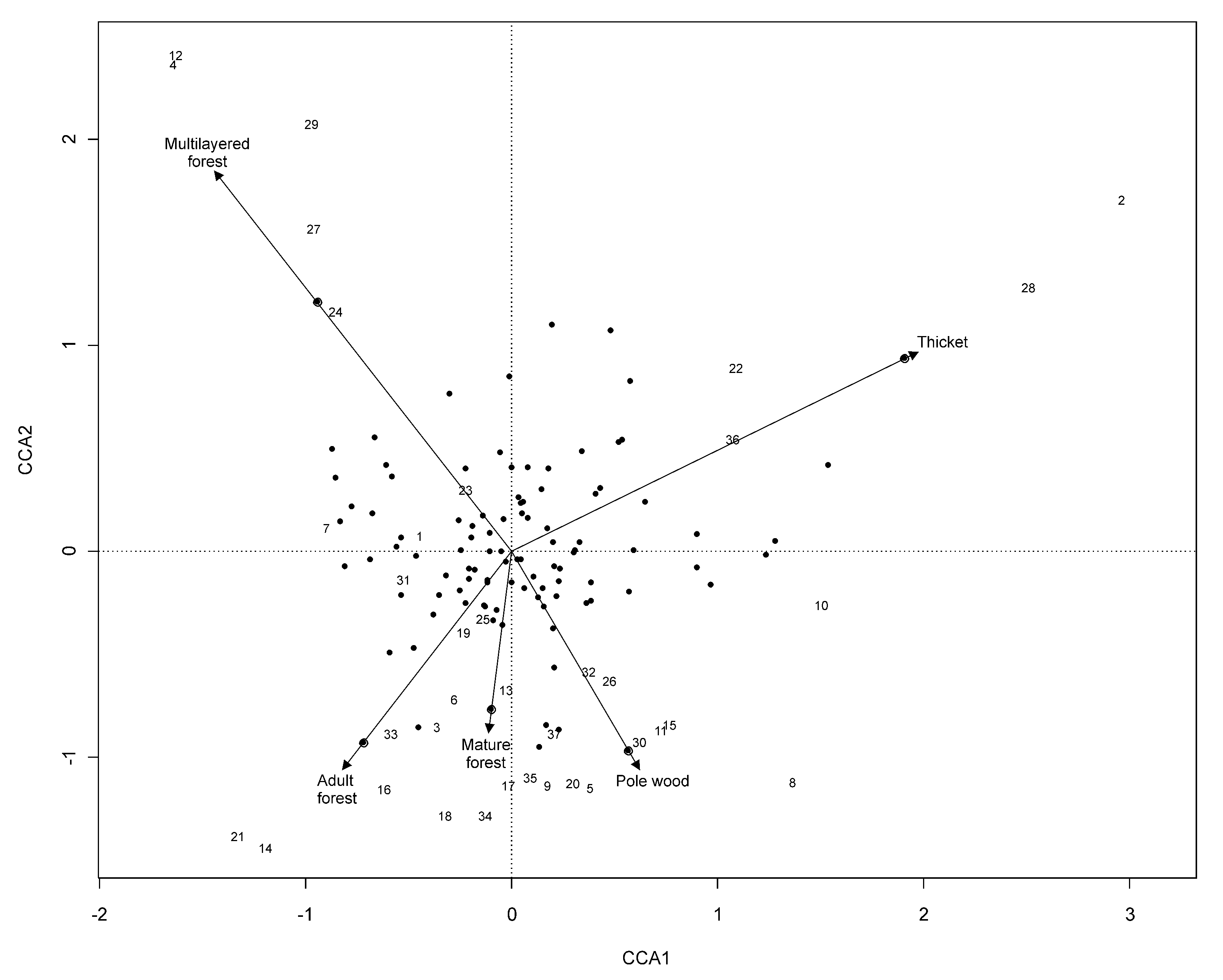
Species scored permitted the discrimination of a set of species strictly related with each LiDAR structure type:
- thicket was characterized by shrub species (e.g., Salix spp, Corylus avellana, Sorbus chamaemespilus);
- multilayer forest was mainly characterized by Orthilia secunda, Festuca altissima, Abies alba (tree level);
- pole wood was characterized by Sorbus aria, Veratrum lobelianum and Lonicera nigra;
- mature forest was characterized by Myosotis sylvatica, Galeopsisi speciosa and Carex sylvatica;
- adult forest was characterized by Neottia nidus-avis, Ranunculus auricomus (aggr.) and Anemone trifolia.
In terms of community characterization, all the stands were ascribable to the association Anemono-Fagetum ([45]), which includes all the Illyrian mixed forests dominated by Fagus sylvatica and Picea abies, developed on limestone of mountain belt of the Querco-Fagetea class ([46]). The connection with the association Anemono-Fagetum was guaranteed by the constant presence of the Vaccinio-Piceetea class elements such as Picea abies, Vaccinium myrtillus, Vaccinium vitis-idaea subsp. vitis-idaea, and Carex alba. The connection with the higher syntaxonomical levels was guaranteed by a large nucleus of characteristics species, such as Luzula sylvatica subsp. sieberi and Polystichum lonchitis of the suballiance (Saxifrago-Fagenion), or Anemone trifolia and Fagus sylvatica for alliace (Aremonio-Fagion) and order (Fagetalia sylvaticae) characteristics.
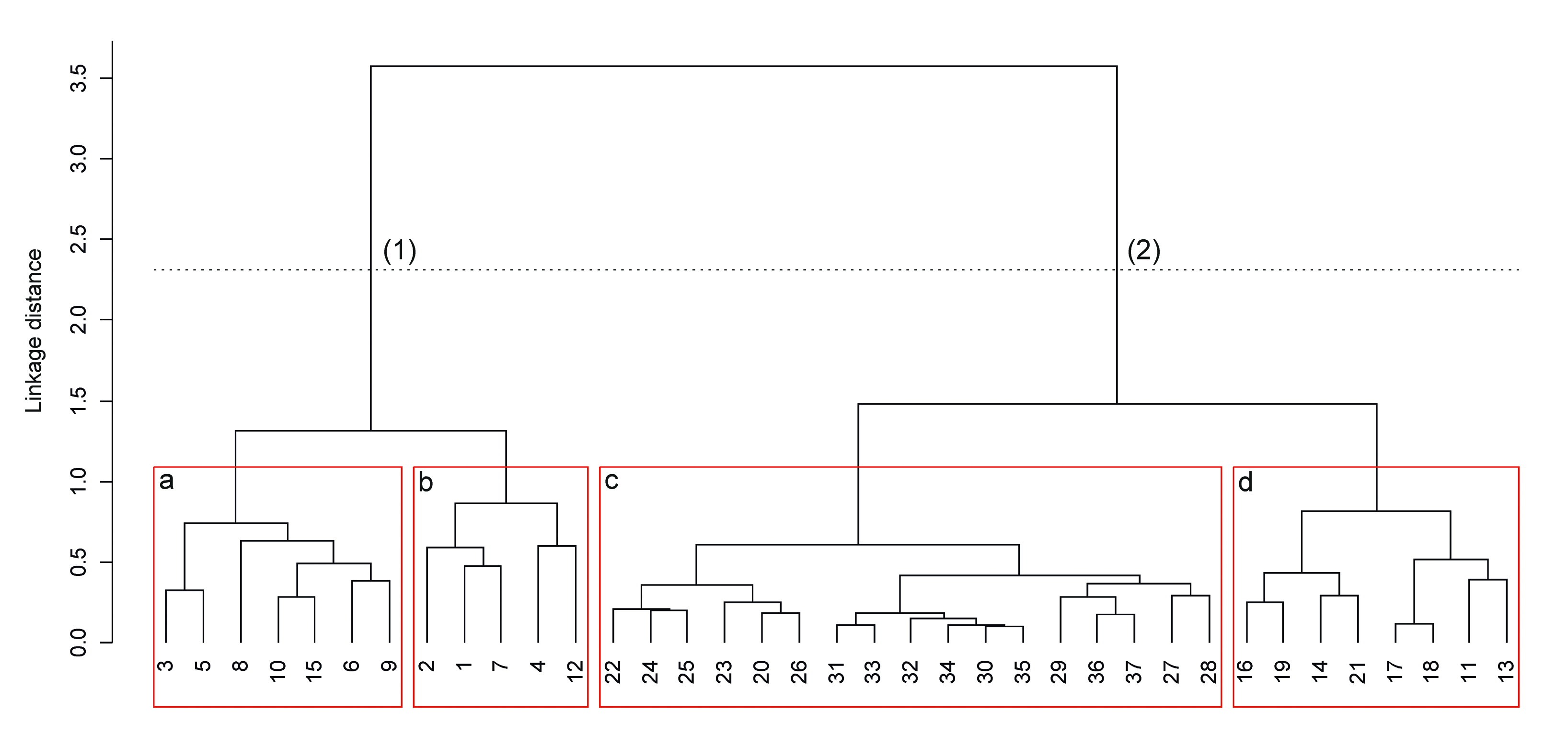
The cluster analysis identified four main groups as variations of the trait plant community (Fig. 10). The identified types confirmed the general homogeneity in the analyzed stands and had not any syntaxonomical significance. However, the separation of these vegetation types represents a contribution for the interpretation of the relationship between structure, dynamics and ecological value of the forest ([28]). Specifically, the cluster tree was split into two main groups: (1) mixed forests on primitive or medium evolved neutral substrates, corresponding mainly to pole wood and multilayer forest, which have low species richness; (2) mixed forests evolved or primitives, rich in species, mainly owing to mature or old forest. Within the first group the following sub-groups were found: (a) pioneer stages with few association and sub alliance characteristic species, depleted floristic richness and ferns richness, and (b) acids evolved soil, with high frequency of blueberries (Vaccinium myrtillus, Vaccinium vitis-idaea subsp. vitis-idaea) and few of sub alliance and order characteristic species. Within the second group the following two clusters were identified: (c) heterogeneous stands with high floristic richness, many characteristics species and participation of Larix decidua, and (d) mature stands with the highest number of characteristics species. Even though the structural classes did not perfectly match with each of the groups obtained from multivariate analysis (Tab. 8), a high correspondence between mature and adult forest stand and vegetation group 2 was pointed out.
Fig. 10 - Cluster dendrogram of vegetation survey (similarity ratio, ward method). (1), (2) = first cut; a, b, c, d = second cut. The numbers indicate sample sites.
Tab. 8 - Cluster groups sharing into LiDAR structural categories. (1), (2): first cut of cluster dendrogram; (a), (b), (c), (d): second cut of cluster dendrogram.
| Groups | (1) | (2) | total | ||||
|---|---|---|---|---|---|---|---|
| a | b | total 1 | c | d | total 2 | ||
| Regeneration phase | - | - | - | - | - | - | - |
| Thicket | 1 | 1 | 2 | 3 | - | 3 | 5 |
| Pole wood | 4 | - | 4 | 3 | 2 | 5 | 9 |
| Adult forest | 1 | - | 1 | 4 | 2 | 6 | 7 |
| Mature forest | - | 1 | 1 | 3 | 3 | 6 | 7 |
| Two-layred forest | 1 | 1 | 2 | - | - | - | 2 |
| Multilayred forest | - | 2 | 2 | 4 | 1 | 5 | 7 |
| Overall | 7 | 5 | 12 | 17 | 8 | 25 | 37 |
Discussion
The most common methods to detect tree vertexes using LiDAR data are based on Canopy Height Models (CHM) created from the difference between a DTM and a Digital Surface Model (DSM - where cell value is the height of the highest laser point). In such cases, a stem is detected for every local maximum of the central cell of a n-sized moving window ([54]), where n can also vary as a function of tree height ([61]). The combined use of LiDAR and multi-spectral image data ([62]), as well as the local maximum of the correlation value between a moving-window template and the CHM above a threshold, has also been already tested ([57]). However, all these methods are heavily dependent on the cell size of the raster models and on the moving window size, which tends to be a limiting factor when applied to complex stand conditions ([66]). On the contrary, the method used in the present paper directly relies on the raw data (points) and has shown a good accuracy in extracting tree vertexes and detecting forest area (land cover map). In term of coniferous/broadleaf map, the main difficulty in distinguishing coniferous from mixed stands was probably due to the higher tree density, which decreases the number of points per crown available for the curve approximation, and/or the low LiDAR posting density (2.8 points m-2), which did not allow us to proper characterize the understory vegetation ([6]). This low post density is typical of not dedicated flight ([13]) and had also an influence in the accuracy of the structure map. A full-waveform (FW) survey would have probably been very supportive: post-processing a full-waveform could have doubled the number of returns ([65]), thus adding information for the cluster analysis and successive classification. It is also documented in literature that low posting density will lead to an underestimation of the tree height metrics, because it is likely that most of the tree vertexes will not be hit by a laser pulse ([51], [47], [61]).
Nilsson ([51]), in a similar study in Sweden (4.0 ha area and 26 plots), explained 78% of the variability in forest stem volume using variables extracted from LIDAR. Previous studies in the Alps demonstrated the existing of correlation between stand volume and mean height derived from LiDAR data ([76], [77]). In the present study, according to model validation, LiDAR-estimated mean height describes up to 58% of volume variability and 62% of carbon stocks variability in agreement with Naesset ([48]). These results can be deemed as positive considering the different forest types, structures and categories considered in this study. However, they also underline the importance for an integration of ground and remotely sensed data to avoid bias in volume estimation, as model parameters are always site-specific.
In terms of plant species composition, all the stands were ascribable to the association Anemono-Fagetum ([45]). The overall biological spectrum agreed with other literature spectra of local mixed deciduous forest ([59], [23]) and the comparison of each biological spectrum with structural categories (Tab. 6) highlighted an overall homogeneity across all structural categories. However, while hemicryptophytes, phanerophytes and chamaephytes did not discriminate LiDAR structural categories, the distribution of geophytes seem to be a good guide group ([34]). In particular, as shown in other forest types ([22], [31], [3]), the abundance of geophytes group is strictly related to the shading degree of the forest stand (i.e., tree density, canopy cover). In our studied stands, this occurs especially in pole wood and adult forest, where the coverage of the canopy reaches its maximum.
The high richness of thicket and multilayered stands was due to the presence of a large number of shrub and herb species coming from open environments (i.e., pastures, alpine prairie and scree pioneer vegetation), as confirmed by the vegetation analysis. This trend may be explained by two different phenomena: (i) involvements of pioneer species in the early phases after forest disturbance (i.e., regeneration after harvest in thicket), in agreement with the intermediate-disturbance hypothesis ([32], [17], [8]); (ii) discontinuous structure of tree cover in multilayered stands, which allows the occurrence of grassland and light-demanding species ([81], [31], [10]). On the other hand, the higher biodiversity, especially in the understory flora, was due to an increase in the complexity for this paraclimax communities, where rare species were more present ([43], [8]). Vegetation type identification obtained through LiDAR structures, CCA and vegetation analysis (cluster) allowed us to detect a set of species that characterized each forest stand. These pools of characteristic species also explained the existence of different ecological features amongst LiDAR structures (e.g., soil evolution, developmental phases of phytocoenoses).
The integration of floristic and phytosociological analyses allowed us to highlight a different contribution of LiDAR structural categories on vegetation characterization. In particular, the classical phytosociological analysis, exclusively focused on the vegetation resemblance, partially explained the variability observed among the LiDAR categories. Indeed, this emphasized the role of other ecological factors in influencing the species composition of each forest structural category that were not considered in this analysis, such as flora natural turnover and forest management.
Conclusions
The forest structure map derived from LiDAR data have proved to be a reliable tool for the characterization of forest stands in areas with an high natural interest if adequately supplemented by field analysis. In particular, the approach used in the present study was able to describe the study area from different points of view, all important for land management and planning. In fact, we were able to distinguish forest from non-forest areas, coniferous from broadleaf or mixed stands and to deeply characterize forest structure. The discrepancies we found between LiDAR forest structure map and ground points was probably due to the low LiDAR posting density (2.8 points m-2), which did not allow to proper characterize the understory vegetation, and relative small ground-plot size (531 m2) in comparison to the minimum LiDAR derived polygon area. LiDAR-estimated mean height was able to describe volume variability in the study area even though the integration of ground data and remotely sensed data is important to avoid bias in the estimation. In terms of vegetation characterization, the present study allowed to highlight the power of LiDAR structural maps to asses biodiversity and to characterize vegetation ecological stability. In particular, LiDAR derived mean heights allowed to characterized different structural phases which, in our case, were mainly related to different successional stages. This strong link between LiDAR structure map and biodiversity is mainly due to the fact that ecological conditions (i.e., light) are mainly influenced by vertical forest structure (i.e., discontinuous structure of tree cover in multilayered stands) and/or disturbance (i.e., regeneration after harvest in thicket). The approach proposed in this paper permitted to discriminate high natural values forest structures, where a careful management is more needed from a conservationist point of view. Moreover, some driver species were identified and related to each structural class.
In conclusion, this study highlights the potential of LiDAR-based approaches for the accurate classification and characterization of forest structures and succession phases in mixed coniferous forests. However, further research should be conducted across different forests types, characterized by different complexity and ecological diversity.
Acknowledgements
The work was funded by Direzione Centrale Risorse Rurali, Agroalimentari e Forestali - Servizio Gestione Forestale e Produzione Legnosa - Regione Friuli Venezia Giulia (Italy) - with a grant for innovation in the field of forest management (ALIFORMIDI project; l.r. 26/2005 art. 16). LiDAR raw data elaboration was performed by e-Laser s.r.l. (⇒ http://www.e-laser.it). The authors would like to thank Stefania Gentili, Elisa Pizzolitto, Giacomo Blasone, Alessandro Merci, Andrea Tabacchi, for the help during field sampling.
References
Gscholar
Gscholar
Gscholar
Gscholar
Gscholar
Gscholar
CrossRef | Gscholar
Gscholar
Gscholar
Gscholar
Gscholar
Gscholar
Gscholar
Gscholar
Gscholar
Gscholar
Gscholar
Gscholar
Gscholar
Gscholar
Gscholar
Gscholar
Gscholar
CrossRef | Gscholar
Gscholar
Gscholar
Gscholar
Gscholar
Gscholar
Gscholar
Authors’ Info
Authors’ Affiliation
F Boscutti
C Bertacco
G De Simon
M Sigura
F Cazorzi
P Bonfanti
Department of Agricultural and Environmental Sciences, University of Udine, v. delle Scienze 206, I-33100 Udine (Italy)
MOUNTFOR Project Centre, European Forest Institute, Via E. Mach 1, San Michele a/Adige, Trento (Italy)
Land, Environment, Agriculture and Forestry Department, CIRGEO - Interdepartmental Research Center on Cartography Photogrammetry - Remote Sensing and G.I.S., University of Padova, Padua (Italy)
Corresponding author
Paper Info
Citation
Alberti G, Boscutti F, Pirotti F, Bertacco C, De Simon G, Sigura M, Cazorzi F, Bonfanti P (2013). A LiDAR-based approach for a multi-purpose characterization of Alpine forests: an Italian case study. iForest 6: 156-168. - doi: 10.3832/ifor0876-006
Academic Editor
Giustino Tonon
Paper history
Received: Nov 12, 2012
Accepted: Feb 11, 2013
First online: Apr 08, 2013
Publication Date: Jun 01, 2013
Publication Time: 1.87 months
Copyright Information
© SISEF - The Italian Society of Silviculture and Forest Ecology 2013
Open Access
This article is distributed under the terms of the Creative Commons Attribution-Non Commercial 4.0 International (https://creativecommons.org/licenses/by-nc/4.0/), which permits unrestricted use, distribution, and reproduction in any medium, provided you give appropriate credit to the original author(s) and the source, provide a link to the Creative Commons license, and indicate if changes were made.

Web Metrics
Breakdown by View Type
Article Usage
Total Article Views: 68126
(from publication date up to now)
Breakdown by View Type
HTML Page Views: 55603
Abstract Page Views: 5305
PDF Downloads: 5365
Citation/Reference Downloads: 68
XML Downloads: 1785
Web Metrics
Days since publication: 4815
Overall contacts: 68126
Avg. contacts per week: 99.04
Article Citations
Article citations are based on data periodically collected from the Clarivate Web of Science web site
(last update: Mar 2025)
Total number of cites (since 2013): 34
Average cites per year: 2.62
Publication Metrics
by Dimensions ©
Articles citing this article
List of the papers citing this article based on CrossRef Cited-by.
Related Contents
iForest Similar Articles
Review Papers
Accuracy of determining specific parameters of the urban forest using remote sensing
vol. 12, pp. 498-510 (online: 02 December 2019)
Review Papers
Remote sensing-supported vegetation parameters for regional climate models: a brief review
vol. 3, pp. 98-101 (online: 15 July 2010)
Research Articles
High resolution biomass mapping in tropical forests with LiDAR-derived Digital Models: Poás Volcano National Park (Costa Rica)
vol. 10, pp. 259-266 (online: 23 February 2017)
Review Papers
Analysis of full-waveform LiDAR data for forestry applications: a review of investigations and methods
vol. 4, pp. 100-106 (online: 01 June 2011)
Research Articles
Estimation of aboveground forest biomass in Galicia (NW Spain) by the combined use of LiDAR, LANDSAT ETM+ and National Forest Inventory data
vol. 10, pp. 590-596 (online: 15 May 2017)
Research Articles
Mapping the vegetation and spatial dynamics of Sinharaja tropical rain forest incorporating NASA’s GEDI spaceborne LiDAR data and multispectral satellite images
vol. 18, pp. 45-53 (online: 01 April 2025)
Short Communications
When a definition makes the difference: operative issues about tree height measures from RPAS-derived CHMs
vol. 13, pp. 404-408 (online: 03 September 2020)
Technical Reports
Detecting tree water deficit by very low altitude remote sensing
vol. 10, pp. 215-219 (online: 11 February 2017)
Research Articles
Classification of xeric scrub forest species using machine learning and optical and LiDAR drone data capture
vol. 18, pp. 357-365 (online: 07 December 2025)
Research Articles
Identification and characterization of gaps and roads in the Amazon rainforest with LiDAR data
vol. 17, pp. 229-235 (online: 03 August 2024)
iForest Database Search
Search By Author
Search By Keyword
Google Scholar Search
Citing Articles
Search By Author
Search By Keywords
PubMed Search
Search By Author
Search By Keyword


