Modeling the fine root biomass dispersion using a special influence function
iForest - Biogeosciences and Forestry, Volume 1, Issue 5, Pages 141-144 (2008)
doi: https://doi.org/10.3832/ifor0469-0010141
Published: Nov 25, 2008 - Copyright © 2008 SISEF
Research Articles
Abstract
This paper presents a successful application of techniques from the adjustment theory for modeling interaction in fine root biomass dispersion. Using special distance and species dependent weightings the influence function for fine root biomass dispersion of two species is estimated. Using the estimated influence functions the fine root biomass is predicted at the locations where the real data was sampled. Goodness of fit of our model is evaluated by comparing sample values and predicted values. However, the results show successful coincidence between sampled and predicted values. Finally, we present an example for the root dispersion in a mixed stand of beeches and spruces in Saxony/Germany.
Keywords
Forest effects, Fine root biomass, Interaction, Influence function
Introduction
Forest scientists as well as wood processing industry are interested in understanding and modeling interactions among trees in stands. The spatial distribution of the resource pool trees rely on affects the availability of these resources like water, nutrients and radiation for a tree. Now, such a characteristic as the fine root biomass depends on locations of the corresponding trees, their interactions and competition effects among them. Investigations of the spatial dispersion of the fine root biomass can contribute to an improved knowledge about these effects. In this paper, the multi-tree case with trees from two different species is discussed. At fixed locations at ground level we want to model the total mean of the fine root biomass in a fixed soil depth belonging to the trees from both species. Obviously, root dispersal is caused by the trees. The total biomass of fine roots consists of the contributions of the individual trees. Here, interactions can affect the root biomass. Therefore, we model the fine root biomass by a weighted sum of individual biomass contributions. Now, the fine root biomass measurements should additionally be weighted related to the relative number of neighbouring trees of the same species. This two-step weighting is necessary for modeling as well intra-specific interactions among trees of the same species as inter-specific interactions between different species. Obviously, our model can also be generalised for more than two species.
There are different mathematical methods for modeling interaction effects, see ([6], [7], [10]). In this paper, techniques of adjustment theory are taken into account.
Material and methods
Study site
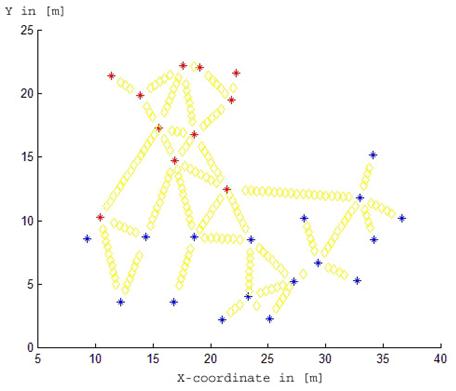
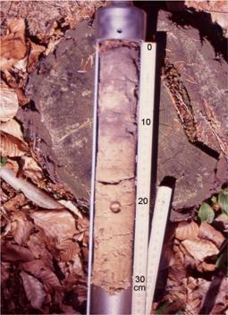
The study was carried out in a mixed spruce and beech stand consisting of 11 beech (species 1) and 17 spruce trees (species 2) in Germany (Saxony) near to Dresden. The study site is part of a greater nearly homogeneous spruce stand. In 2003, soil cores were taken at 226 given sampling points with collections of the fine root biomass from the forest floor organic and mineral horizon, see Fig. 1 and Fig. 2.
Fig. 1 - Locations of trees and fine root biomass measurements (transects) at the Rabenau site. The trees of the first species (beech) are coloured with red stars. The trees of the second species (spruce) are coloured with blue stars. Yellow diamonds show locations of measurements. Both axes X and Y are in [m].
Sampling procedure started with the collection of roots from the forest floor organic and mineral horizons using a steel frame (diameter 50 mm). The samples per core hole (organic horizon, mineral soil up to a depth of 80 cm) were filled in separated plastic bags. According to ([2]) only roots <= 2 mm diameter are classified as fine roots. These roots were selected irrespective of their shape. Finally, the dead roots were separated. The distinction between living and dead components was made according to Murach ([5]). Following separation, samples of live roots were oven-dried at 65°C for 96 h. Mycorrhizae was not separated from root material.
In Näther & Wälder ([7]) an approach based on fuzzy theory is proposed for modeling inter- and intra-specific aggregations. In Näther & Wälder ([6]) a statistical model for dispersion effects based on cluster point processes is discussed. Ammer & Wagner ([1]) present an approach for modeling the mean fine root biomass of Norway spruce stands. Especially, they restricted themselves to modeling fine root biomass of one species. Here, we present an alternative method for modeling the fine root biomass distribution of two species. Techniques of the adjustment theory are used for our modeling.
Mathematical methods
A deterministic alternative to the mark correlation function discussed in Wälder & Wälder ([10]) is the so called influence function defined in Wälder ([11]). The utilisation of tree individual-based models has been established in forest research and management for some years now. Analogously to the influence function many other models make use of the zone of influence (“ZOI” sensu [3]) approach; but they utilise this approach in very different ways ([12], [8], [9], [4]). Now, such an influence function approach provides a simple method for interaction analysis and its advantage relies on its rejection of embarrassing restrictions which are necessary for stochastic methods: For example, it is well-known that not any function can be a correlation or a density function. Some conditions have to be fulfilled.
Let us explain the main idea of the influence function method based on an example from forestry. We assume that each tree characteristic, for example the fine roots biomass, depends not only on the corresponding tree, but also on other trees, namely on their locations and characteristics. It seems to be realistic to assume that this influence only depends on distances between measurement points of fine roots biomass and the tree. We denote the maximal tree distance with still existing influence f with parameter R. Therefore, f(r) = 0, r > R holds. In our case study we use R=10 and R = 15 [m]. Now, we assume that this function f is identical for all trees of the same species in a stand.
Further, we assume that there are two tree species with two different fine root biomass influence functions. The measurements of fine root biomass are taken around each tree following radial transect lines. The whole plot is divided into two groups: fine root biomass from trees of the first and of the second species, see Fig. 1.
The next model assumption refers to the linearity of the average of individual influences of neighbouring trees for a fine root biomass value. Let mj be the fine root biomass of species j, j = 1, 2, at point x0 . If N neighbouring trees are located at xi, i = 1, …, N, then we use the following approach assuming that all distances are smaller than R (eqn. 1):
The weights w in eqn. 1 are necessary because the number of trees still increases with increasing distance. Now, these influence functions fj , j = 1, 2 have to be estimated using the sampled fine root biomass values mj. The estimator is denoted by fj. Our approach to solve this problem is based on techniques from the adjustment theory. At first, we restrict the number of unknown variables in eqn. 1. For example, for five values of the influence function this corresponds to the following locations (eqn. 2):
Tab. 1 - Some statistical characteristics providing goodness-of-fit of our model.
| R | Species | Observed measurements |
Values estimated with m=5 |
m=7 | m=9 | |
|---|---|---|---|---|---|---|
| 10 [m] | Species 1 | Mean | 60.9248 | 60.9561 | 60.8873 | 61.5880 |
| Variance | 4.7628 x 10³ | 1.7635 x 10³ | 1.7387 x 10³ | 1.8707 x 10³ | ||
| Correlation | 1.0 | 0.6152 | 0.6107 | 0.6395 | ||
| Species 2 | Mean | 97.2478 | 99.9726 | 98.3769 | 98.4068 | |
| Variance | 1.3658 x 10⁴ | 0.7236 x 10⁴ | 0.7660 x 10⁴ | 0.8045 x 10⁴ | ||
| Correlation | 1.0 | 0.7513 | 0.7567 | 0.7712 | ||
| 15 [m] | Species 1 | Mean | 60.9248 | 61.6426 | 61.9068 | 61.809 |
| Variance | 4.7628 x 10³ | 1.7532 x 10³ | 2.0310 x 10³ | 2.1523 x 10³ | ||
| Correlation | 1.0 | 0.6031 | 0.6575 | 0.6768 | ||
| Species 2 | Mean | 97.2478 | 100.317 | 98.61 | 98.794 | |
| Variance | 1.3658 x 10⁴ | 0.7072x 10⁴ | 0.7729 x 10⁴ | 0.7558 x 10⁴ | ||
| Correlation | 1.0 | 0.7297 | 0.7583 | 0.7522 | ||
We should note that another number of unknown variables in eqn. 1 can also be considered. Tab. 1 presents the results for m = 5, 7 and 9 in our case study. Setting (eqn. 3):
leads to m values of rk , k = 1, …, m. Let us mention that an increasing number of unknown variables firstly results in an increasing estimation error and secondly in oscillations of the influence function estimator fj caused by the relatively small number of trees at a fixed distance from a measurement. Thus, this restriction to only five (seven or maximal nine) variables seems to be useful and necessary. To take into account the stem diameter the parameter rmin > 0is needed. Using seven or nine variables does not change the form of influence functions significantly, see Tab. 1. Thus, in eqn. 4 and eqn. 5 we use m = 5 only in order to avoid overloading the given relations.
At second, each measurement mj should be weighted additionally. This weighting should mirror our confidence in the corresponding measurement. It means that the accuracy of a measurement mj (and in the same time our confidence) increases significantly, if there are only trees of the same species j. We denote these weights with p. Each weight should be proportional to the relative number of trees of the same species the considered measurement of fine root biomass belongs to.
The solution of the following linear system of equations eqn. 4 which is well-known in the adjustment theory leads to the estimation fj of the corresponding influence functions for both tree species j=1, 2 (eqn. 4).
where n is the number of measurements of fine root biomass denoted with M for both tree species j, and (eqn. 5)
The elements of the matrix A are cumulative weights which are defined in eqn. 1. The weights of all trees located at distances closer to the corresponding rk , k = 1, …, 5 should be summed up.
The exact solution of eqn. 4 corresponds then to (eqn. 6):
Results
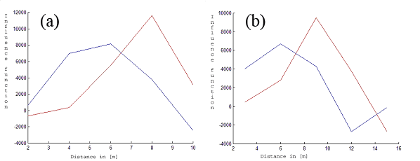
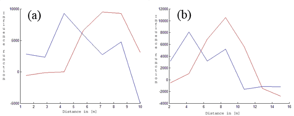
We applied the method described above for our data. From Fig. 3 and Fig. 4 it can be seen that the maximum of fine root biomass is different for both species. The maximum of fine root biomass for a beech yields approx. 5 [m], while a spruce has this maximum at approx. 8 [m]. We restricted ourselves to R = 10 [m] and 15 [m] because of the small size of the observation window.
Fig. 3 - Fitted fine root biomass influence functions (Y-axis). The red lines correspond to the first tree species (beech). The blue lines describe the estimated influence function for the second tree species (spruce) for k = 5 and R = 10 [m] (a) and R = 15 [m] (b). The X-axis represents the distance in [m].
Fig. 4 - Fitted fine root biomass influence functions (Y-axis). The red lines correspond to the first tree species (beech). The blue lines describe the estimated influence function for the second tree species (spruce) for k = 7 and R = 10 [m] (a) and R = 15 [m] (b). The X-axis represents the distance in [m].
It should be noted again that using more than 5 variables does not change the form of the influence functions significantly. The corresponding results can be seen in Tab. 1.
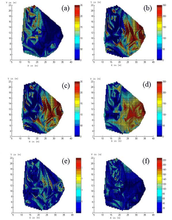
Fig. 3 and Fig. 4 show the estimated influence functions for some parameters. Fig. 5 presents the comparison between real and estimated values of fine root biomass for k=5 and R=15 [m]. The linear interpolation method is used for visualisation of the results in the observation window.
Fig. 5 - Real measurements of fine root biomass for the first species (a) and for the second species (b) at Rabenau. Estimated fine root biomass for the first species (c) and for the second species (d) for k=5, R=15 [m]. Absolute difference between observed and estimated values for the first species (e) and for the second species (f). Both axes X and Y are in [m]. The colour scale represents the fine root biomass in [mg/cm3].
Discussion
In our paper we show that intra- and inter-specific interaction and competition effects among trees and species can be modeled by a special two-step weighting approach. From an ecological point of view this is necessary because forest dynamics is shaped by suppression, support and survival of the strongest species.
In general, a mathematical model is a problem-related simplification and requires some restrictions and assumptions. Goodness-of-fit should be proved for each model. In our approach two influence functions are estimated. Based on them, the values of fine roots biomass are predicted at the locations where real measurements are given. The comparison of real (observed) and predicted (model) values is carried out calculating their means, variances and the correlation between real and model values. The obtained results underline that our model is well suited for describing the fine root dispersion in a mixed stand of two species.
Conclusions
Applying the influence function approach is very helpful, especially for such cases if additional restricting demands of other mathematical approaches could not be satisfied. For example, there are too small sampling sizes or vague measurements, etc. An influence function is free from restrictions: It can be as well positive as negative, it is not normalized. It is a simple and meaningful tool for a preliminary analysis of spatial multidimensional data.
Our approach provides a more general and flexible approach in comparison with the approaches by Näther & Wälder ([7]) and Ammer & Wagner ([1]). Differently from Ammer & Wagner ([1]) our model is not restricted to one species. The approach presented in this paper can even be generalized by using more than two species of trees. Differently from Näther & Wälder ([7]) our approach renounces strict statistical model assumptions.
Further, other tree-dependent characteristics, which are of interest for forest scientists, can be analyzed in a similar way. Therefore, we want to contribute to the broader dissemination of our approach in forestry and ecological research.
Acknowledgements
The authors are grateful to S. Wagner and A. Zeibig, who collected the root data we used.
References
Gscholar
Gscholar
Gscholar
Gscholar
Gscholar
Authors’ Info
Paper Info
Citation
Wälder O, Wälder K (2008). Modeling the fine root biomass dispersion using a special influence function. iForest 1: 141-144. - doi: 10.3832/ifor0469-0010141
Paper history
Received: Apr 01, 2008
Accepted: Oct 30, 2008
First online: Nov 25, 2008
Publication Date: Nov 25, 2008
Publication Time: 0.87 months
Copyright Information
© SISEF - The Italian Society of Silviculture and Forest Ecology 2008
Open Access
This article is distributed under the terms of the Creative Commons Attribution-Non Commercial 4.0 International (https://creativecommons.org/licenses/by-nc/4.0/), which permits unrestricted use, distribution, and reproduction in any medium, provided you give appropriate credit to the original author(s) and the source, provide a link to the Creative Commons license, and indicate if changes were made.
Web Metrics
Breakdown by View Type
Article Usage
Total Article Views: 50235
(from publication date up to now)
Breakdown by View Type
HTML Page Views: 42148
Abstract Page Views: 3204
PDF Downloads: 3836
Citation/Reference Downloads: 54
XML Downloads: 993
Web Metrics
Days since publication: 6339
Overall contacts: 50235
Avg. contacts per week: 55.47
Article Citations
Article citations are based on data periodically collected from the Clarivate Web of Science web site
(last update: Mar 2025)
Total number of cites (since 2008): 3
Average cites per year: 0.17
Publication Metrics
by Dimensions ©
Articles citing this article
List of the papers citing this article based on CrossRef Cited-by.
Related Contents
iForest Similar Articles
Research Articles
Fine root production and distribution in the tropical rainforests of south-western Cameroon: effects of soil type and selective logging
vol. 3, pp. 130-136 (online: 27 September 2010)
Research Articles
Effects of understory removal on root production, turnover and total belowground carbon allocation in Moso bamboo forests
vol. 9, pp. 187-194 (online: 20 November 2015)
Research Articles
Fine root morphological traits and production in coniferous- and deciduous-tree forests with drained and naturally wet nutrient-rich organic soils in hemiboreal Latvia
vol. 16, pp. 165-173 (online: 08 June 2023)
Research Articles
Analysing interaction effects in forests using the mark correlation function
vol. 1, pp. 34-38 (online: 28 February 2008)
Research Articles
Effects of nitrogen loading under low and high phosphorus conditions on above- and below-ground growth of hybrid larch F1 seedlings
vol. 11, pp. 32-40 (online: 09 January 2018)
Research Articles
Mid-rotation fertilization and liming of Pinus taeda: growth, litter, fine root mass, and elemental composition
vol. 14, pp. 195-202 (online: 24 April 2021)
Research Articles
Short-term recovery of fine root carbon stock is inhibited by skid trails in a humid tropical forest
vol. 18, pp. 344-349 (online: 30 November 2025)
Research Articles
Properties and prediction accuracy of a sigmoid function of time-determinate growth
vol. 8, pp. 631-637 (online: 13 January 2015)
Research Articles
Carbohydrate metabolism during new root growth in transplanted Larix olgensis seedlings: post-transplant response to nursery-applied inorganic fertilizer and organic amendment
vol. 10, pp. 15-22 (online: 22 September 2016)
Research Articles
Thinning effects on soil and microbial respiration in a coppice-originated Carpinus betulus L. stand in Turkey
vol. 9, pp. 783-790 (online: 29 May 2016)
iForest Database Search
Search By Author
Search By Keyword
Google Scholar Search
Citing Articles
Search By Author
Search By Keywords
PubMed Search
Search By Author
Search By Keyword

