Modeling aboveground carbon in flooded forests using synthetic aperture radar data: a case study from a natural reserve in Turkish Thrace
iForest - Biogeosciences and Forestry, Volume 17, Issue 5, Pages 277-285 (2024)
doi: https://doi.org/10.3832/ifor4527-017
Published: Sep 27, 2024 - Copyright © 2024 SISEF
Research Articles
Abstract
Flooded forests are rare and highly dynamic ecosystems, yet they can store a significant amount of carbon because of their ability to produce biomass rapidly. Estimation and mapping of the carbon that is stored in flooded forests are challenging tasks through the use of optical remote sensing because these ecosystems are often located in moist regions where clouds can interfere with data acquisition and image interpretation. This study models the aboveground carbon (AGC) stocks of a flooded forest in Turkish Thrace with synthetic aperture radar (SAR) data, which are less affected by weather and illumination conditions compared to optical imagery. Forest management plan data, including inventory records of 229 sample plots, a detailed forest cover map, and stand tables of the 2.119-ha Igneada Longoz Forest, were used to calculate AGC and to develop spatially explicit models based on ALOS/PALSAR-2 (Advanced Land Observing Satellite/Phased Array L-band Synthetic Aperture Radar) and Landsat-8 images. The results indicated that the horizontally transmitted and horizontally received (HH) and cross-polarization ratio (CPR) bands of ALOS/PALSAR were the most influential variables in the linear and nonlinear regression models. The models did not include any variables from either radar- or optical-based vegetation indices. While the estimation accuracies of the two models were similar (root mean square percentage error ≈ 26%), the linear model yielded negative estimations in several land cover classes (e.g., dune, forest opening, degraded forest). AGC stock was estimated and mapped using the nonlinear model in these cases. The density map revealed that Igneada Longoz Forest stored 279,258.9 t AGC, with a mean and standard deviation of 124 ± 115.4 t C ha-1. AGC density varied significantly depending on stand types and management units across the forest, and carbon hotspots accumulated in the northern and southern sites of the study area, primarily composed of ash and alder seed stands. The models and maps that this study developed are expected to help in the rapid and cost-effective assessment of AGC stored in flooded forest ecosystems across the temperate climate zone.
Keywords
SAR Mosaics, Landsat-8, Normalized Difference Vegetation Index (NDVI), Aboveground Biomass and Carbon Stocks, Carbon Density Maps, Bottomland Forests, National Parks, Igneada
Introduction
Flooded forests (e.g., floodplain forests, alluvial forests, freshwater swamp forests or longoz in Turkish) are highly dynamic ecosystems that are generally located on water-rich lowlands and river valleys near the sea ([17], [33], [8]). These ecosystems have a strong relationship with flood events as they need newly deposited sediment sites for natural regeneration. Every flood changes the landscape mosaic by destroying a part of existing stands and opening favorable sites for new ones; as a result, such lands are sometimes called mobile mosaics ([17]).
Globally, flooded forests are rare, with European examples nearly eliminated due to human activity. The remaining ones are in critical condition and are listed as a priority forest habitat type in the European Habitats Directive Annexes (Directive 92/43/ EEC 1992 - [10]). These ecosystems are also important due to their rich biodiversity ([17]). Junk ([20]) state that more than 20% of tree species in the Amazon Basin are located in flooded forests. In Turkey, longoz forests are flooded during winter and spring seasons, providing vital habitat for migrating birds ([6]) such as black woodpecker (Dryocopus martius), white-tailed eagle (Haliaeetus albicilla), and fish eagle (Pandion haliaetus). As a result, Igneada Longoz Forests National Park has been identified as one of the Important Bird and Biodiversity Areas (IBA) in Turkey ([13]).
Significantly, flooded forests serve as appreciable aboveground carbon (AGC) sinks due to their rapid biomass production capacity ([7]). The high level of productivity is closely linked to the flood waters that convey large amounts of organic matter from upper watersheds ([16]). These organic materials are deposited on floodplains and fertilize soil resources with minerals. The plant community becomes naturally fertilized ([17], [8]). In flooded forests, seasonal water levels often change significantly due to hydrological processes such as rainfall, infiltration, and evapotranspiration ([23]). These processes may alter forest dynamics and distribution patterns which cause considerable variations in carbon sequestration rates. Accurate estimation and periodic monitoring of existing carbon stocks, AGC in particular, are essential for the sustainable management of these ecosystems under the climate change challenge ([46], [23]).
Researchers often prefer remote sensing data rather than relying solely on field measurements to estimate wall-to-wall coverage of forest biomass ([2]) and carbon density ([47]). A correlative relationship between the field-based inventories and remote sensing images can be established for regional-based aboveground biomass (AGB) maps ([14]). Optical, radar, and LiDAR remote sensing systems have been used to estimate biomass for differing forest types. In optical systems, spectral vegetation indices have shown their potential over the Calabrian pine forests of Turkey ([32]), and the woodland of the tropical West African Sahel Savanna ([1]). However, the estimation accuracy of optical systems remained moderate (coefficient of determination <0.50), due to numerous shortcomings, such as the lack of vertical information on forest cover, which is critical for estimating AGB. Other shortcomings include the occlusion effects of clouds and smoke ([14]), limited spectral information provided by high resolution (i.e., < 5 m) images ([2]), shaded areas over canopy gaps ([24]), and the saturation issue particularly arising in densely-vegetated areas ([37]). Still, some research findings suggest that specific vegetation indices, such as normalized difference vegetation index (NDVI), may improve AGB and AGC modeling performance in certain circumstances when used as supplementary data ([22], [1], [2]).
Airborne LiDAR has also been used to characterize the vertical canopy structure of canopies. Essentially, airborne LiDAR technology provides more accurate data than optical and radar satellites ([49]); however, compared to satellite data, the coverage of area that is offered by this source is often limited. Perhaps more importantly, this technology is still costly and is not widely available in many countries ([25], [14]). The recent availability of spaceborne LiDAR data, such as what is provided by NASA’s Global Ecosystem Dynamics Investigation (GEDI) and Ice Cloud and Land Elevation Satellite-2 (ICESat-2) missions, offer new opportunities to forest biometricians. While these missions are capable of characterizing the vertical forest structure with certain accuracy rates, their sample-based nature and insufficient data density do not allow their use alone for wall-to-wall estimates of forest attributes at stand and landscape levels ([11], [45]). Thus, researchers often combine spaceborne LiDAR data with other remote sensing sources.
Synthetic Aperture Radar (SAR) systems, on the other hand, are less susceptible to rainy and cloudy weather than optical satellite images, and they are able to collect data during night and day. Moreover, some SAR systems offer publicly available data to researchers for using in scientific studies. Long wavelength SAR, which can partially penetrate through the forest canopy, is a good predictor for forest biomass ([5], [31]). Currently, L-band is the longest wavelength that is provided by satellite systems, and mosaic ALOS/PALSAR (Advanced Land Observing Satellite/Phased Array L-band Synthetic Aperture Radar) data is currently available free of charge. The 25-m-resolution mosaic data were used to assess the AGB of coniferous forests in Turkey ([44]), tropical forests in Mexico ([14]), deciduous forests of northern India ([31]), mixed forests in China ([25]), and Cameroon’s savannas ([27]). Besides the polarimetric information of the data, different arithmetic combinations (e.g., cross-polarization ratio - CPR, radar vegetation index - RVI) from SAR images may also show higher sensitivity to vegetative cover ([31], [3]). While the European Space Agency (ESA) plans to make the first P-band BIOMASS and L-band ROSE-L SAR satellite products available, the Japanese Aerospace Exploration Agency’s (JAXA) ALOS/PALSAR-2 mosaics are still one of the few SAR products ready-to-use to date.
The present study modeled and mapped AGC that was stored in flooded forests by using ALOS/PALSAR-2 products and NDVI data. This focus was realized by meeting the following objectives: (i) calculating AGC based on ground measurements of forest plots and the stand-type map; (ii) developing statistical models for estimating AGC by using ALOS/PALSAR-2 and NDVI datasets as independent variables; and (iii) generating AGC stocking maps for the entire forest area. The final models, maps, and conclusions from this study are expected to support the management of flooded forests as well as carbon accounting efforts.
Material and methods
Study area
The study area is the Igneada Longoz (flooded) Forests on the Black Sea coast near the Bulgaria-Turkey border (Fig. 1). The area was established in 2007 as a national park because of its rare and sensitive ecosystems. The total area of the park is 3156 ha that hold unique ecosystems, including natural longoz forests (2119 ha), coastal dunes (113 ha), lagoon lakes (34 ha), swamps, and riparian areas ([13]). The longoz forests are surrounded by moderate slopes that are covered by mixed deciduous stands. Ash (Fraxinus angustifolia subsp. oxycarpa), hornbeam (Carpinus betulus, C. orientalis), oak (Quercus robur subsp. robur), maple (Acer campestre), linden (Tilia argentea), beech (Fagus orientalis) and alder (Alnus glutinosa subsp. glutinosa) species dominate the forested lands and generally form mixed stands in the poletimber (i.e., 8 < DBH < 19.9 cm) and thin-tree (20 < DBH < 35.9 cm) developmental stages. In the forest management plan of Igneada ([13]), the forestlands are wholly allocated for ecological and socio-cultural functions, which indicates that the management objective is not timber production. Nevertheless, a limited annual allowable cut (1260 m3 as thinning) has been determined for the oak-dominated management unit.
Fig. 1 - Location and land-use/land-cover classes of the study area over ALOS imagery.
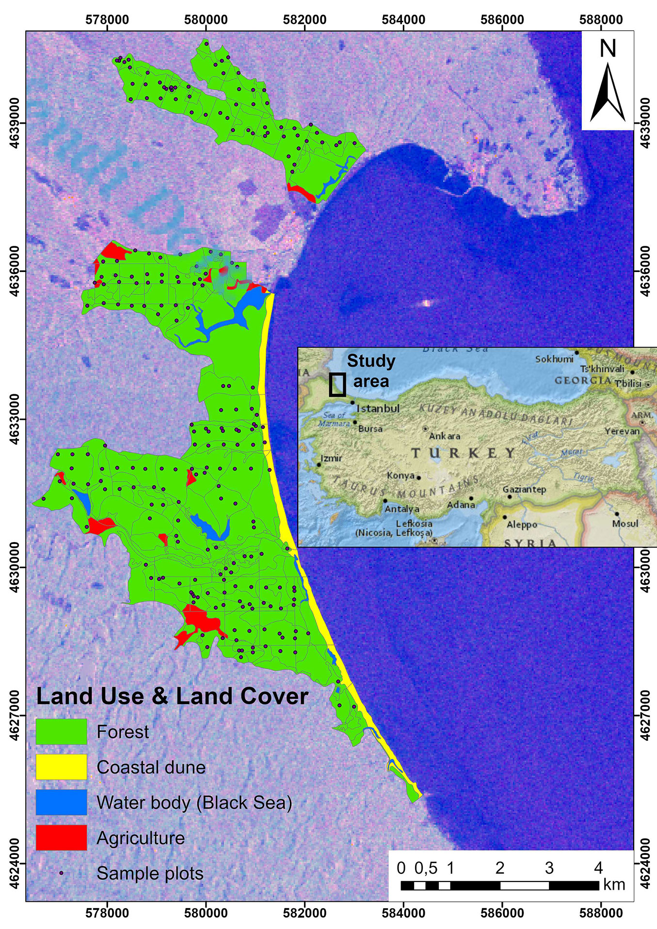
The region’s climate is generally moist, rainy, and cool. According to the records from the nearest meteorological station, the average air temperature and annual precipitation are 12.0 °C and 818 mm, respectively. Alluvial and limeless brown forest soils are the most prevalent soil types in the study area. Four endemic, 12 rare, and 55 medicinal plant species survive in Igneada. These species include Silene sangaria, Crepis macropus, Centaurea kilaea, Aurinia uechtritziana, Pancratium maritimum, and Ruscus aculeatus ([6], [33]).
The study area is also rich in terms of herbs, shrubs, and understory. While Humulus lupulus, Periploca greaca, Tamus communis subsp. cretica, Hedera helix, Sambucus nigra, and Sorbus aucaparia species are prevalent in forested lands, Leymus racemosus subsp. sabulosus, Matthiola fruticose, and Cyperus capitatus exist in the coastal dunes. The lagoons, swamps, and riparian areas, on the other hand, provide favorable sites for wetland species, including Phragmites australis, Cladium mariscus, Schoenoplectus lacustris subsp. tabernaemontani, Althea officinalis, and Dipsacus laciniatus ([13]). Some of these species can make fieldwork challenging when they are prevalent on the forest floor.
Fieldwork, calculation of forest carbon, and aggregation process
In order to calculate the AGB and AGC of the study area, we use field data that was measured from 220 sample plots. The plots were located by using a recreational-grade handheld GPS that had a positional accuracy around 5 m. The shape of the plots was circular with differing sizes (i.e., 400, 600 or 800 m2) according to the canopy cover of the sampled plot. Tree species were first identified, and then their DBH was measured in each plot to calculate stem volume by using species-specific local volume tables in the forest management plan ([13]). Based on the stem volumes, the AGB of each tree was calculated by using the national biomass conversion and expansion factors (BCEFs) and biomass expansion factors (BEFs - [41]). BEFs and standard wood density values were used for the conversion if BCEFs were unavailable for a given tree species. The species-specific wood densities were compiled from several sources ([15], [18], [19], [40], [41]).
Next, the AGB of individual trees was aggregated to the plot level by totaling all AGB values in each plot. Here, we only considered trees that had a DBH of >7.9 cm as suggested by the Turkish planning rule. Plot-level AGB values were then converted to a unit area (i.e., per hectare) based on the given plot size. Afterward, the default value for the carbon fraction of deciduous species ([19]) was used to calculate AGC per hectare using eqn. 1 ([19]):
where C is the total carbon in the aboveground forest biomass (t C), V is the stand volume (m3 ha-1), BCEFs is the biomass conversion and expansion factor for expanding the stand volume to AGB (t m3), and CF is the carbon fraction of dry matter. The descriptive statistics for field data and calculated AGC values can be seen in Tab. 1.
Tab. 1 - Descriptive statistics for the field data collected from 220 sample plots.
| Forest attributes (plot level) | Descriptive statistics | |||
|---|---|---|---|---|
| Min | Mean | Max | Std. dev. | |
| Tree density (# ha-1) | 275 | 779 | 2050 | 428 |
| Timber volume (m3 ha-1) | 26.0 | 299.0 | 915.9 | 173.9 |
| Aboveground carbon (t C ha-1) | 9.5 | 107.2 | 326.1 | 61.1 |
The sample plots were distributed across 212 sub-compartments (patches), encompassing 41 distinct stand types. To consolidate the plot-level AGC data, the AGC values within the same stands were averaged, allowing for aggregation at both the patch and stand-type levels. This aggregation process was facilitated using the Generalization tool, specifically the dissolve function, within ArcGIS Pro® v. 3.0. For details on the aggregated data and plot-level AGC information, please refer to the Supplementary material (Tab. S1).
SAR data processing
The Advanced Land Observing Satellite (ALOS) Phased Array L-band Synthetic Aperture Radar (PALSAR-2) annual mosaic data for 2016 was used for the analysis. The data was provided as 1×1 degrees in latitude and longitude tiles with a 25 m spatial resolution. Two tiles that cover the study area were obtained from the JAXA. The data had both HH and HV polarizations with gamma-naught values. The pre-processing steps were applied by JAXA. The ALOS World 3D (AW3D30) Digital Elevation Model was used for the geometric correction. The digital numbers were converted to backscatter coefficients (γ°) in decibel (dB) units using eqn. 2:
where γ° is the backscatter coefficient, DN is the digital number of amplitude SAR data, and CF is the calibration factor which is -83 dB ([36]).
We also calculated five variables that were derived from arithmetic combinations of γHH and γHV backscatter coefficients. The calculated variables can be seen in Tab. 2. Thus, statistical relationships between the variables and AGC values were modeled as shown below.
Tab. 2 - ALOS PALSAR-2 polarizations and their derived variables ([29], [26], [3]).
| Polarizations and independent variables used for modeling | Abbreviation | Assigned bands |
Equations |
|---|---|---|---|
| Horizontally transmitted and horizontally received | HH | B1 | n/a |
| Horizontally transmitted and vertically received | HV | B2 | n/a |
| Cross Polarization Ratio | CPR | B3 | γHV / γHH |
| Radar Vegetation Index | RVI | B4 | 4 × γHV / ( γHH + γHV ) |
| Horizontal Dual De-Polarized Index | HDDP | B5 | ( γHH + γHV ) / γHH |
| Normalized Difference Polarization Index | NDPI | B6 | ( γHH - γHV ) / ( γHH + γHV ) |
| Cross Polarization Difference | CPD | B7 | γHH - γHV |
Statistical analysis and modeling
Fig. 2 - The workflow for the statistical analysis and modeling methods.
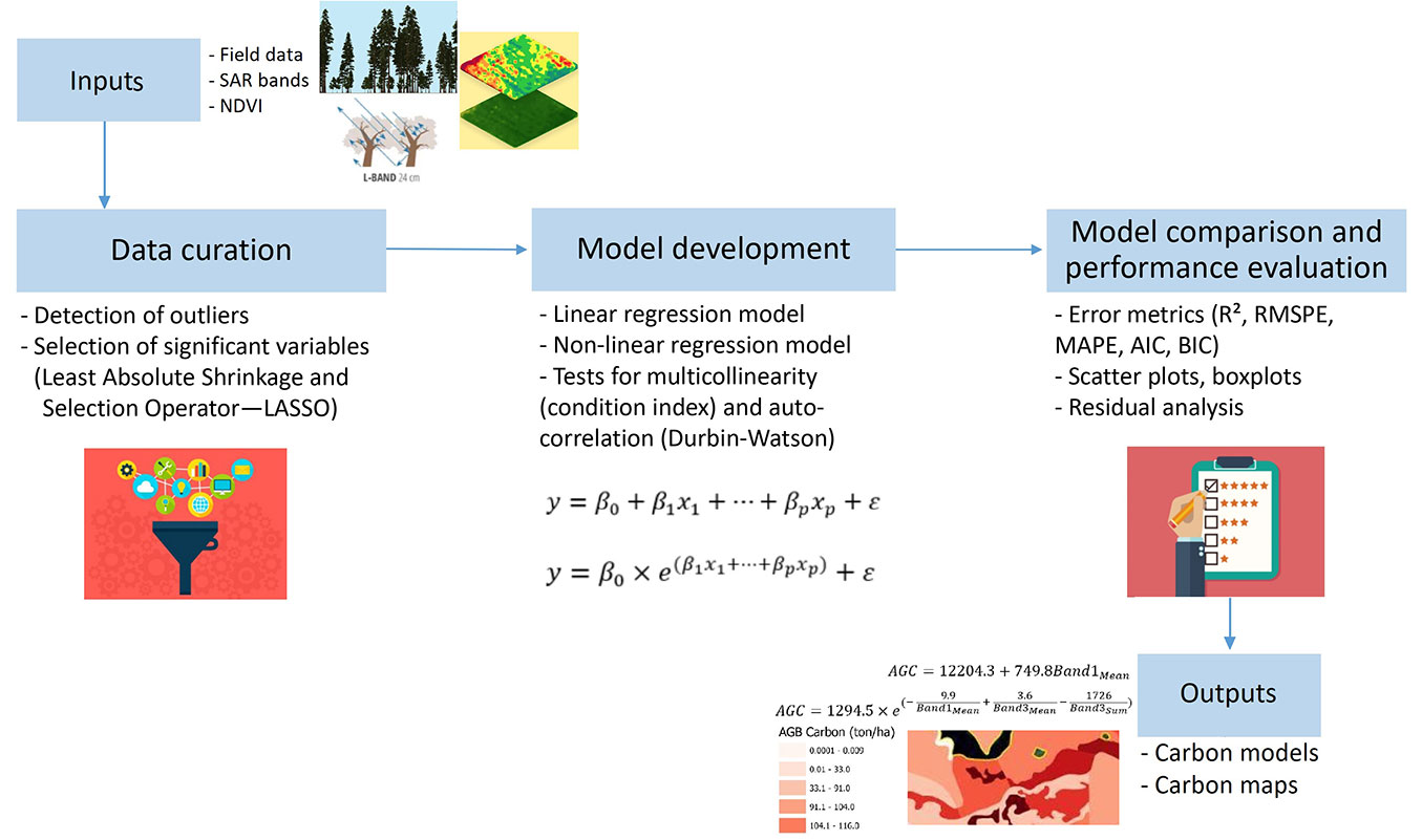
Fig. 2 includes the main steps of the statistical analyses and modeling process. Prior to constructing a predictive model for AGC, we performed the Least Absolute Shrinkage and Selection Operator (LASSO) technique to determine unnecessary variables ([39] - eqn. 3). The LASSO technique attempts to minimize prediction bias by selecting a small number of independent variables. The selection of independent variables in this technique is based on Lambda (λ) value. As λ increases, the number of independent variables decreases, but this reduction may lead to an increase in prediction bias. Conversely, as λ decreases, the number of independent variables increases, which may induce poor performance. In this study, the optimum λ value that provided the best combination of independent variables was determined using 10-fold cross-validation (eqn. 3):
where N is the number of observations, yi is the response variable, xi is the independent variable, β is the regression coefficient to be estimated, T is a pre-specified parameter that determines the degree of regularization, and λ is a regularization parameter.
In the subsequent step, we employed the stepwise variable selection method to establish a linear regression model (LRM - eqn. 4). This method was chosen as it facilitates the evaluation of various combinations of independent variables using model evaluation criteria, such as mean squared error and the Akaike information criterion. Additionally, a nonlinear regression model (NLRM) was developed utilizing the independent variables from the LRM (eqn. 5). The model parameters were estimated based on area-weighted AGC values (n=41):
where ε is assumed to be independent and identically distributed.
The variables that had a p-value lower than 0.05 were determined to be significant. During the fitting of LRM and NLRM, outliers were assigned by using Cook’s Distance (CD) method ([30]), and they were excluded from the data set. After the models were developed, their results were further evaluated based on statistical assumptions, including collinearity and homogeneity ([50]). While the Condition Index (CI) was used to examine collinearity, the homogeneity in the residuals was analyzed by using a plot of residuals versus fitted values with a loess curve. All statistical analyses were performed with MATLAB software.
The performance of LRM and NLRM was compared using common fit indices, including the mean percentage error (Bias% - eqn. 6), root mean square percentage error (RMSPE - eqn. 7), Akaike information criterion (AIC - eqn. 8), and Bayesian information criterion (BIC - eqn. 9). Their mathematical descriptions can be seen in eqn. 6 to eqn. 9:
where yOi and yPi are i-th observed and fitted values, respectively; yMean is the average of observations, N and k are the numbers of observations and parameters, respectively; and L is the log-likelihood value of the fitted model.
NDVI data and GIS analysis
NDVI is a popular vegetation index that represents vegetation health and density based on the difference between the near-infrared and red bands of multispectral optical images ([42]). In order to improve AGC model accuracy, NDVI layers of the study area were generated by using 30-m-resolution Landsat-8 images acquired on 19 June and 6 August 2013. Three essential points were considered in determining these dates: (i) matching the time of the forest inventory campaign (during the summer of 2013) and image acquisition; (ii) downloading cloudless image sets as far as possible; and (iii) representing the leaf-on season of hardwood species in the study area. NDVI was calculated by using the Raster Functions tool of ArcGIS Pro® with eqn. 10 ([42]):
where NDVI is the normalized difference vegetation index (ranges from -1 to 1, unitless), NIR is the near-infrared band of the satellite images (Band 5, in our case), and RED is the red band of the satellite images (Band 4).
Regarding spatial modeling, the aggregated AGC data layer (see above) was overlaid onto NDVI and composite SAR datasets. Pixel values from nine bands (including NDVI layers and those listed in Tab. 2) were extracted based on stand boundaries using ArcGIS Pro’s Zonal Statistics tool, employing both mean and sum functions. Subsequently, the summary tables were integrated into the attribute table of the sub-compartment layer. This process facilitated the correlation of calculated AGC values with NDVI and SAR data, forming the basis for model development.
After model development, the spatial distribution of AGC was mapped only for forest areas based on the stand-type map. AGC density was colorized using the quantile method found in ArcGIS Pro’s Symbology tab.
Results
AGC modeling
The results of LASSO showed that 11 of 17 independent variables were significant (see the upper part of Fig. S1 in Supplementary material). Specifically, Band1Mean, Band1Sum, Band2Sum, Band3Mean, Band3Sum, Band4Mean, Band6Mean, Band6Sum, Band7Sum, NDVIJune, and NDVIAug were statistically important variables, though Band2Mean, Band4Sum, Band5Mean, Band5Sum, and Band7Mean were negligible.
The results of CD showed that 3 of 41 observations were extreme, so these values were discarded from the data set. The LRM and NLRM developed in this study are represented by eqn. 11 and eqn. 12, respectively:
While all estimated parameters were significant at the 0.05 significance level, the values of CI showed no relationship among independent variables.
This study also determined the main effect of each selected variable on predictions of AGC. As seen in Fig. S2 (Supplementary material), Band3Sum was the most influential variable, whereas Band1Mean and Band3Mean had similar magnitudes but opposite effects.
The model fit indices suggested that both the LRM and NLRM had similar prediction success. Although RMSPE, AIC, and BIC values indicated that LRM performed slightly better than NLRM, the Bias% values suggested the opposite outcome (Tab. 3). Additionally, scatter plots depicting fitted versus observed AGC values for both models revealed somewhat different distribution patterns (Fig. 3). While there was generally good agreement between the fitted and observed values, LRM unexpectedly resulted in a few negative predictions.
Tab. 3 - Model fit statistics for linear regression model (LRM) and nonlinear regression model (NLRM).
| Criterion | LRM | NLRM |
|---|---|---|
| Bias (%) | -25.88 | 24.46 |
| RMSPE (%) | 24.00 | 24.75 |
| AIC | 679.46 | 698.49 |
| BIC | 686.01 | 705.14 |
Fig. 3 - The plots of observed versus predicted values of LRM (a) and NLRM (b). The dotted red line represents the 1:1 line, while the black line indicates the regression line.
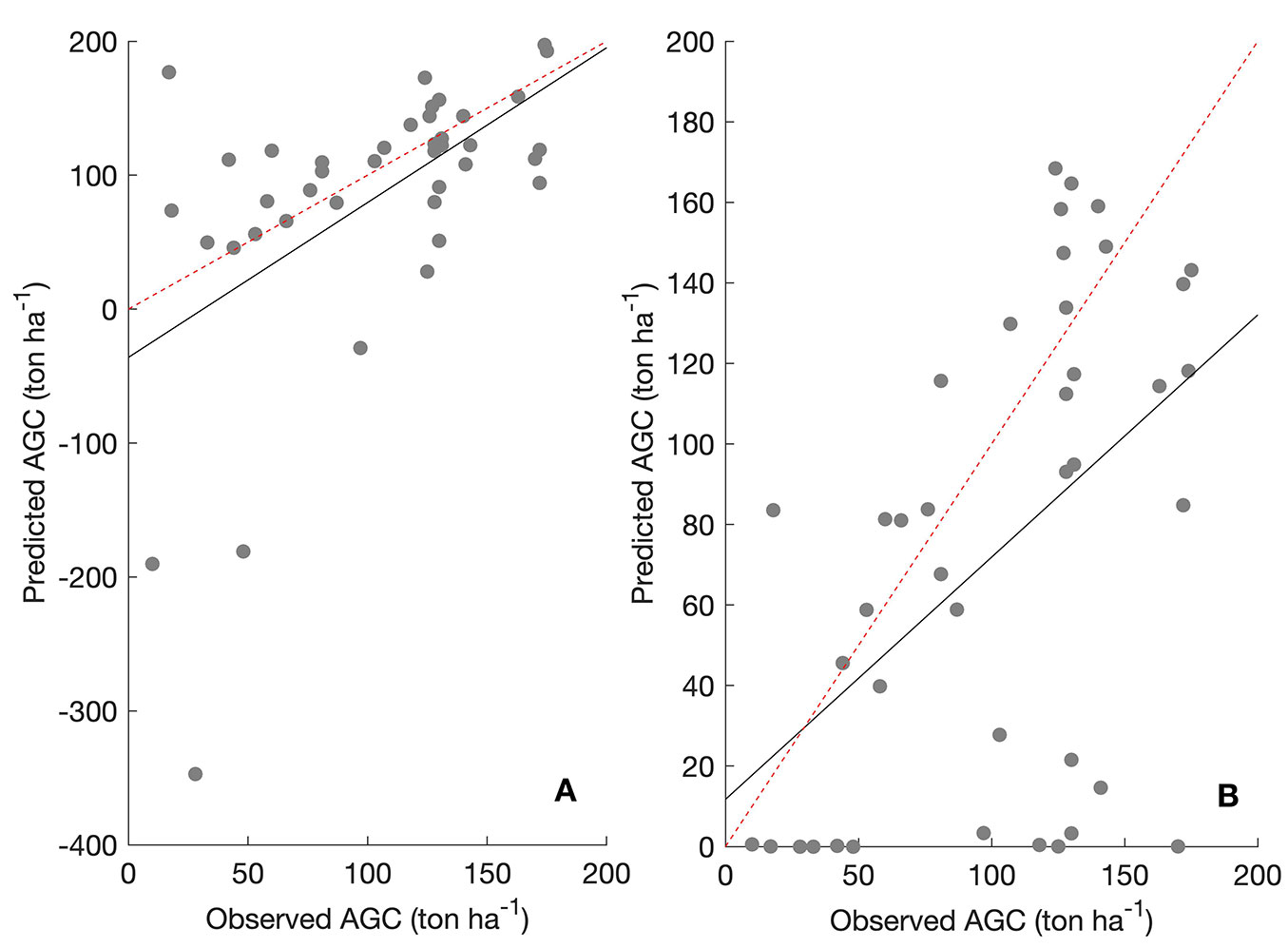
Based on the results from Tab. 3and considering its simple model structure, we generated an AGC map with the LRM. However, LRM yielded negative AGC values for several stands. For these stands, we used NLRM estimates in the AGC map, which is shown and discussed in the next sections. We also included a comparison of fitted versus observed AGC values for pure and mixed stands (Fig. S3 in Supplementary material). The box-and-whisker plots revealed that the model tended to overestimate AGC in both pure and mixed stands; however, the overestimation was more pronounced in mixed stands.
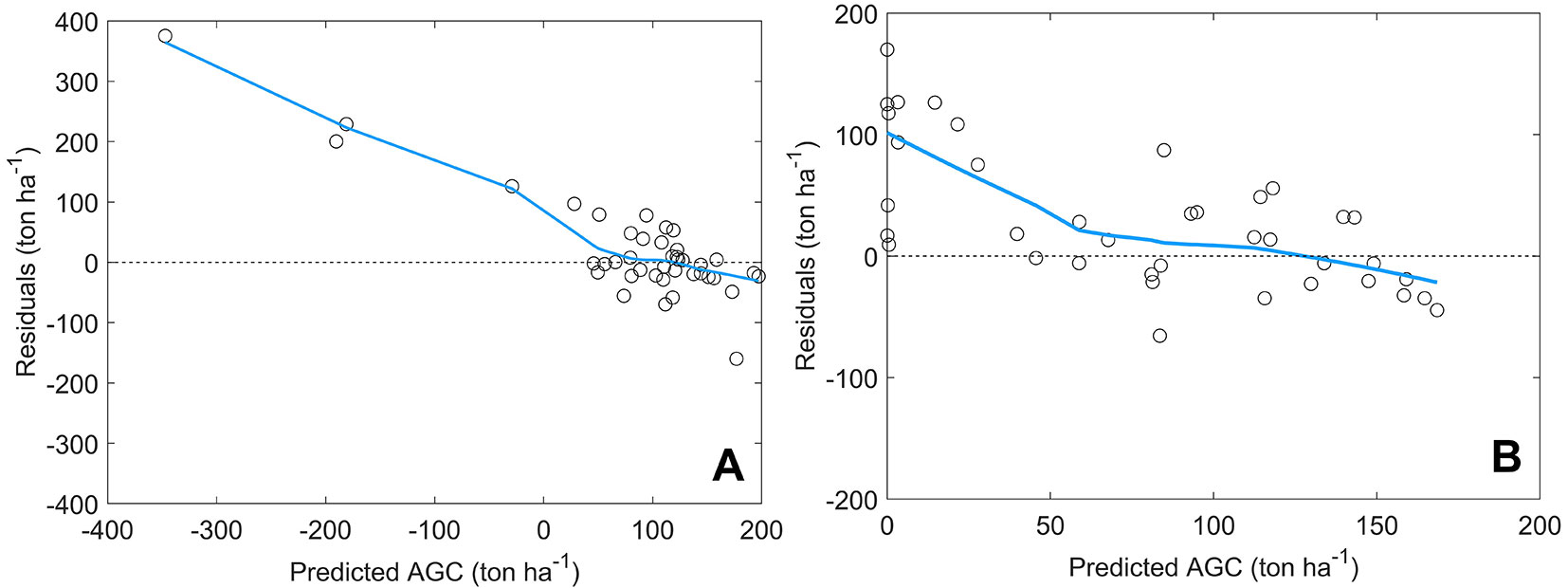
The presence of a heteroscedastic pattern was examined by plotting residuals versus fitted values (Fig. 4). As depicted in the figure, LRM and NLRM exhibited a heteroscedastic tendency for the residuals, which was attributable to the datasets having a limited number of samples. Detailed plot and sub-compartment level predictions of AGC can be found in Tab. S1 (Supplementary material).
Fig. 4 - The plots of residuals versus fitted values with a loess curve for LRM (A) and NLRM (B).
AGC mapping
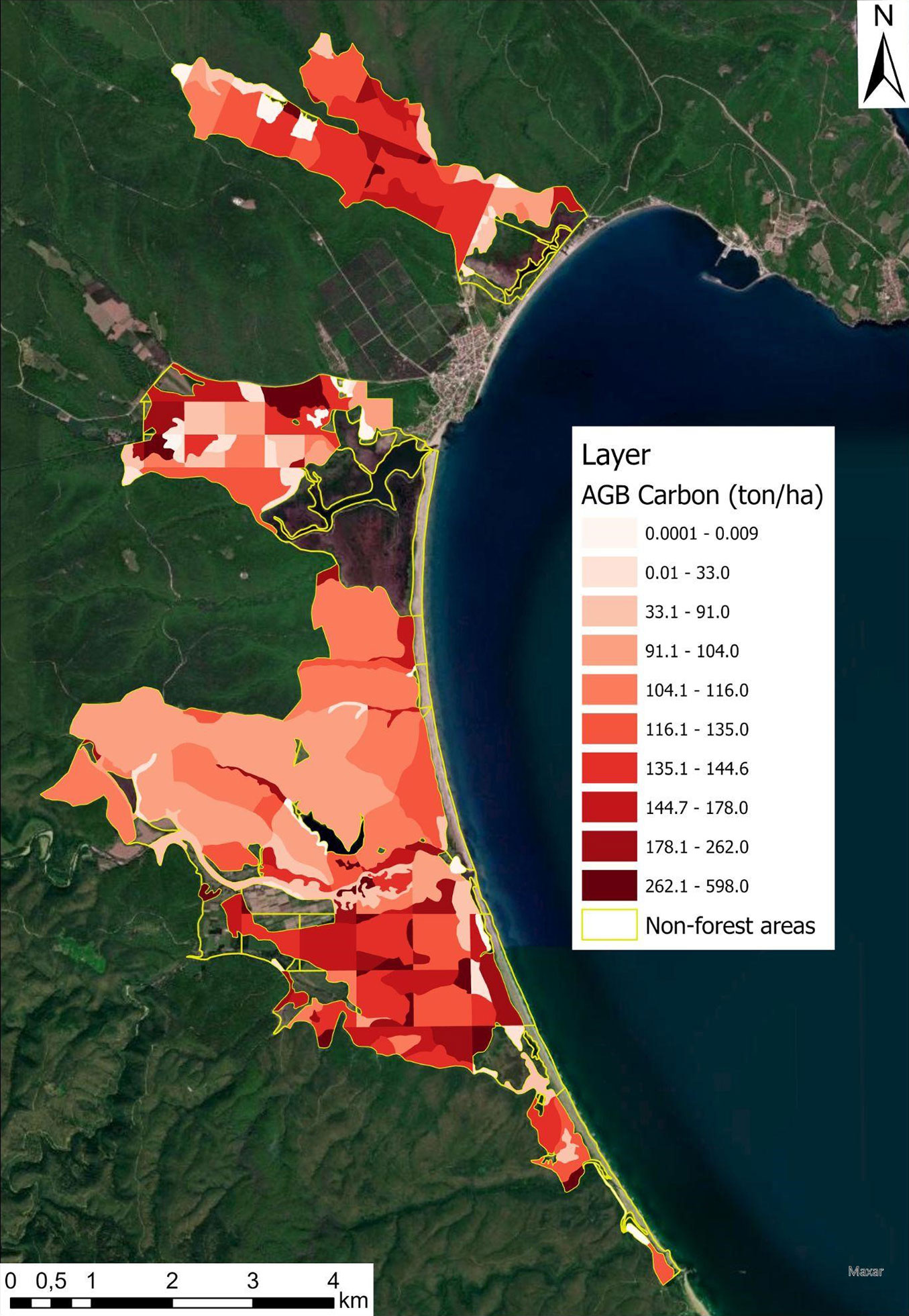
Fig. 5 shows the AGC density and its spatial distribution across the landscape. The map was created by using the models based on SAR data at the sub-compartment level. Accordingly, Igneada Longoz Forests stored 279,258.9 t AGC with a mean and standard deviation of 124.0 ± 115.4 t C ha-1 (Tab. 4). The carbon storage in the forest significantly varied depending on stand type and management unit, which resulted in a non-homogeneous pattern on the map. The forests in the southern and northern portions of Igneada generally stored more carbon than the central areas. The amount of AGC in these hotspots was often higher than 250.0 t C ha-1. The hotspots were partly composed of mixed seed stands of ash and alder species, particularly in the southern portion. Other hotspots included mixed stands of hornbeam, ash, and elm species.
Fig. 5 - Aboveground carbon density map of the Igneada Longoz Forests National Park, Turkish Thrace.
Tab. 4 - Estimated aboveground carbon (AGC) content for forestlands of the Igneada Longoz Forests National Park.
| Stats | AGC amount |
|---|---|
| Min (t ha-1) | 0.1 |
| Mean (t ha-1) | 124 |
| Max (t ha-1) | 598 |
| Std. Dev. (t ha-1) | 115.4 |
| Total (t) | 279,258.9 |
According to the scale that is visible in the legend of the carbon density map (Fig. 5), the central parts of the study site seem to store a moderate amount of AGC per unit area. However, these parts are generally composed of pure stands of oak with large area coverage. Therefore, the relative contribution of AGC in these areas to the total stock was critical. We observed some degraded stands along the Bulanikdere creek (south part of the area), which stored little biomass carbon (7-30 t C ha-1) in their aboveground components. There were also some forest stands storing almost no carbon because they were in the early successional development stages. These stands had naturally regenerated in newly deposited sediment sites after flood events, so they had no considerable biomass in their thin stems (DBH < 8 cm - white irregular patches in Fig. 5). The non-forest areas with some woody species were excluded from the analysis. They were shown transparently on the map because we had no reliable ground data for those areas.
Discussion
In the present study, the total AGC stock in Igneada Longoz Forests was estimated to be about 280 thousand tons with a mean of 124 t C ha-1. To the best of our knowledge, there is no published work reporting AGC values for this region, except for GDF ([13]). Forest planning team reported the mean AGC stock of Igneada as 95.6 t C ha-1 based on forest inventory information which they gathered during the management plan renewal process ([13]). The difference between the mean values likely stems from distinct calculation methods and coefficients used. While we employed species-specific biomass conversion and expansion factors, the management plan utilized standard stem density values and a broad categorization system. This system classifies forests as either coniferous or broadleaved based on the dominant tree species in each stand. However, flooded forests often exhibit multi-species characteristics, with basal area shares that are similar among species. In our case, most stands had more than two species, as evident in Tab. S1 (Supplementary material). This finding corroborates the work of Schöngart et al. ([35]), which emphasizes the importance of developing species-specific allometric models for biomass estimations to reduce error biases.
Much of the published research on flooded forests has been centered in Brazil, underscoring the significant role of the Amazon in carbon cycling. For instance, Borges Pinto et al. ([7]) investigated a Cerrado forest, primarily situated in northern Brazil, reporting mean AGC values of 88 and 92 t C ha-1 for the years 2014 and 2019, respectively. They emphasized the Cerrado biome’s potential as a crucial carbon sink due to its aboveground woody biomass. Similarly, Kauffman et al. ([21]) estimated a mean AGC of 72 t C ha-1 for the semiarid northeast part of the Amazon region. The relatively low amount of AGC can be attributed to sparse vegetation cover in their study area as this region is often called Amazonian savannahs ([9]). While the AGC estimates from Brazil’s flooded forests are comparable to those reported in the present study, we acknowledge significant ecological differences between temperate and tropical forest types. Therefore, careful considerations was given when selecting each case to highlight similarities with our forest area in terms of stand structure. For example, Schöngart et al. ([35]) conducted a comprehensive study focusing on a forest stand with mean DBH and tree height values of 38.3 cm and 17 m, respectively. These values closely resemble a typical stand in Igneada Longoz Forests, as evidenced from stand tables ([13]). The researchers estimated the mean AGC of that stand as 97.2 t C ha-1. The higher estimate reported in our study (124 t C ha-1) can be attributed to differences in forest management regimes, as Igneada has been a national park under strict protection for decades ([6], [33], [13], [8]).
As in any landscape, past anthropogenic disturbances can profoundly influence the spatial structure of flooded forests. Many researchers have reported a high variance in and a heterogeneous distribution of AGB and AGC amounts in their areas of investigation ([43], [14]). Therefore, comparing only the mean amounts may be inadequate or misleading for assessments at the landscape level. For example, Van Pham et al. ([43]) classified their carbon density map into five classes - from very low (0-50 t C ha-1) to very high (200+ t C ha-1) accumulation - and attributed the very-low and the low-stocked areas with bareland after cutting down and newly planted forests in Thuan Chau district, Vietnam. Their results indicated that carbon accumulation values could be as high as 19 times between certain forest types, such as evergreen broadleaf and mixed bamboo forests. In a more recent study from Mexico, land management practices appeared to have a considerable impact on the spatial pattern of AGB and carbon stocks across the landscape ([14]). While the lower stocked areas distributed around agricultural and urban regions, the high-stocked areas were located in strictly protected forestlands. Interestingly, the largest uncertainty was found in the intermediate areas that have store AGB of 25-50 t ha-1. Our carbon density map revealed similar results to those reported by the aforementioned studies. AGC stored in mature broadleaf stands was 17-fold greater than that stored in newly-regenerated oak stands. The spatial pattern was also non-homogeneous in our case. When Fig. 5 is examined, one can clearly see the neighbouring patches with regularly shaped edges that exhibit considerable differences in AGC content. It seems that these differences are likely related to past harvesting activities realized until the area was designated as a national park in 2007. Before 2007, clearcutting was the common practice in the study area, especially for oak stands managed under the coppice system ([13]). Although our field and remote sensing datasets were collected several years later, the disturbance history of the Igneada Longoz Forests was partially detectable in the carbon density map.
In the modeling stage, we had 17 independent variables to estimate the AGC stock in our study area. Among these variables, HH and CPR (HV/HH) were found to be most influential and were used in regression models. Although statistically significant, NDVI and many other SAR indices’ influences on model performance were weak and thus, they were disregarded. Using HH and CPR data as independent variables, 92% of the total variation in AGC content was explained by NLRM. Avtar et al. ([5]) also made reasonable forest biomass estimates by using cross-polarized SAR data in Cambodia. The authors suggested the use of ALOS/PALSAR data for national-level deforestation analyses over tropical regions in the context of REDD+ (Reducing Emissions from Deforestation and forest Degradation) programs. Similarly, Ningthoujam et al. ([31]) used mosaic ALOS/PALSAR data to estimate the biomass of tropical deciduous mixed forests in northern India. Using the HH, HV, and SAR-derived indices, they found that HH polarization and HV provided the most accurate estimates. Among the variables that they used, the sum of polarizations yielded similar estimation accuracy to the use of HH solely. In another study, Ma et al. ([25]) used mosaic data of ALOS/PALSAR to estimate forest AGB in China. In their NLRM, HH had more influence on model accuracy than the sum of polarization (HH+VV) and HV data. With regard to mixed forests, the influence of the dual polarimetry (HH/HV) ratio was lower than in other data sets. These results are partly in line with the present case from Turkey. In our case, HV/HH ratio played the most critical role in both LRM and NLRM, perhaps due to the different foci and species mixtures of the two studies. Ma et al. ([25]) focused on AGB while our focus was on AGC. Also, their mixed forests were composed of hardwood and softwood species. These differences imply that the remotely sensed data needed to estimate forest biomass and forest carbon may differ although AGC is usually derived from woody biomass. Another implication is that backscatter coefficients of coniferous and deciduous trees can be dissimilar in each SAR band, so researchers should test many band combinations in their modeling efforts. It is also noted that the use of additional variables from image texture may improve the estimation results in SAR-based forest monitoring and assessment studies ([48]).
Regarding AGC mapping, we basically used the LRM because the error metrics of the two models were similar, and use of the NLRM in GIS would be challenging due to the complex structure of nonlinear equations compared to simple LRM. Although LRMs have been extensively used in remote sensing of forest attributes ([34], [28]), the models’ abilities to explain observed data patterns are rarely examined. Among a few studies, Fleming et al. ([12]) have cautioned researchers about the potential for LRMs to yield negative values in relation to the estimation of forest attributes through remote sensing. Archontoulis & Miguez ([4]) suggest the use of NLRMs to address the disadvantages of LRMs, such as high sensitivity to outliers. Similarly, Sun et al. ([38]) stated that NLRMs are more appropriate if unreasonable estimates (e.g., negative carbon stock) occur in remote sensing projects. Because of these suggestions and experiences from previous research, we used NLRM to estimate the AGC of forest stands with biologically unrealistic estimates. The AGC map in Fig. 5 was based on two models; basically, LRM was used, but NLRM estimates were inserted into some land cover classes that had negative AGC values. These classes included dune, agriculture, marsh, forest opening, and a few forest stands. Thus, no negative values were observed on the AGC map. While this approach may be perceived as a limitation of the study, it can also be viewed as a novel aspect contributing to the production of more realistic carbon maps.
Conclusions
This study utilized forest inventory data and SAR images to model the AGC of Igneada Longoz Forests, situated along the Black Sea coastline in northwestern Turkey. The key findings revealed that the AGC stock of flooded forests could be estimated and mapped with an RMSPE of approximately 26% using various combinations of bands from ALOS/PALSAR alone. Given the dynamic nature and rarity of flooded forests, monitoring the spatial and quantitative changes in their AGC stocks is of value and SAR data can aid in forest planning and land management efforts by offering a rapid and relatively straightforward solution for carbon assessment. The importance of such assessments is expected to increase further, particularly as voluntary carbon offset markets are set to be established in the Turkish forestry sector soon.
List of Abbreviations
AGB: Aboveground biomass; AGC: Aboveground carbon; AIC: Akaike information criterion; ALOS: Advanced land observation satellite; BCEF: Biomass conversion and expansion factors; BIAS%: Percentage bias; BIC: Bayesian information criterion; CD: Cook’s distance; CF: Carbon fraction; CI: Condition Index; CPD: Cross polarization difference; CPR: Cross-polarization ratio; DBH: Diameter at breast height (1.3 m); GDF: Turkish General Directorate of Forest; HDDP: Horizontal dual de-polarized index; HH: Horizontally transmitted and horizontally received; HV: Horizontally transmitted and vertically received; IBA: Important bird and biodiversity areas; JAXA: Japanese Aerospace Exploration Agency; LASSO: Least absolute shrinkage and selection operator; LRM: Linear regression model; NDPI: Normalized difference polarization index; NDVI: Normalized difference vegetation index; NLRM: Nonlinear regression model; PALSAR: Phased array type L-band synthetic aperture radar; REDD+: Reducing emissions from deforestation and forest degradation; RMSPE: Root mean square percentage error; RVI: Radar vegetation index; SAR: Synthetic aperture radar.
Acknowledgments
The authors would like to express their sincere gratitude to writing tutors of the University of Georgia (UGA) for improving the final version of the manuscript in terms of English styles and grammar. Additionally, we would like to acknowledge the Turkish General Directorate of Forestry (GDF/OGM) for providing us with data in relation to forest management plans in a digital format.
Author Contributions
CV conceived the study, drafted the original manuscript, and generated the final maps; FB performed the statistical analyses, developed the models; SA processed satellite data, calculated vegetation indices; PPA calculated carbon stocks; CS arranged and corrected field inventory data collected from sample plots. All of the authors helped to write and edit the final manuscript.
Funding
This research did not receive any specific grant from funding agencies in the public, commercial, or not-for-profit sectors.
Declaration of Competing Interest
The authors declare that they have no known competing financial interests or personal relationships that could have appeared to influence the work in this paper.
Data Availability
The ALOS-PALSAR data was provided by Japan Aerospace Exploration Agency (JAXA) and downloaded from ⇒ https://www.eorc.jaxa.jp/ALOS/en/dataset/fnf_e.htm
References
CrossRef | Gscholar
CrossRef | Gscholar
Gscholar
Gscholar
CrossRef | Gscholar
Gscholar
Gscholar
Gscholar
Gscholar
Gscholar
CrossRef | Gscholar
Gscholar
Gscholar
CrossRef | Gscholar
Authors’ Info
Authors’ Affiliation
Faculty of Forestry, Artvin Coruh University, 08100 Artvin (Turkey)
Warnell School of Forestry and Natural Resources, University of Georgia, Athens 30602, GA (USA)
Faculty of Forestry, Çankiri Karatekin University, 18200 Çankiri (Turkey)
Department of Geomatics Engineering, Hacettepe University, Sihhiye, Ankara (Turkey)
Department of Geography, University of Bonn, 53115 Bonn (Germany)
Forestry Research and Application Center, Artvin Coruh University, 08100 Artvin (Turkey)
Corresponding author
Paper Info
Citation
Vatandaslar C, Bolat F, Abdikan S, Pamukcu-Albers P, Satiral C (2024). Modeling aboveground carbon in flooded forests using synthetic aperture radar data: a case study from a natural reserve in Turkish Thrace. iForest 17: 277-285. - doi: 10.3832/ifor4527-017
Academic Editor
Matteo Garbarino
Paper history
Received: Nov 24, 2023
Accepted: Jun 28, 2024
First online: Sep 27, 2024
Publication Date: Oct 31, 2024
Publication Time: 3.03 months
Copyright Information
© SISEF - The Italian Society of Silviculture and Forest Ecology 2024
Open Access
This article is distributed under the terms of the Creative Commons Attribution-Non Commercial 4.0 International (https://creativecommons.org/licenses/by-nc/4.0/), which permits unrestricted use, distribution, and reproduction in any medium, provided you give appropriate credit to the original author(s) and the source, provide a link to the Creative Commons license, and indicate if changes were made.

Web Metrics
Breakdown by View Type
Article Usage
Total Article Views: 15116
(from publication date up to now)
Breakdown by View Type
HTML Page Views: 10341
Abstract Page Views: 2489
PDF Downloads: 1892
Citation/Reference Downloads: 0
XML Downloads: 394
Web Metrics
Days since publication: 646
Overall contacts: 15116
Avg. contacts per week: 163.80
Article Citations
Article citations are based on data periodically collected from the Clarivate Web of Science web site
(last update: Mar 2025)
Total number of cites (since 2024): 1
Average cites per year: 0.50
Publication Metrics
by Dimensions ©
Articles citing this article
List of the papers citing this article based on CrossRef Cited-by.
Related Contents
iForest Similar Articles
Research Articles
Remote sensing of Japanese beech forest decline using an improved Temperature Vegetation Dryness Index (iTVDI)
vol. 4, pp. 195-199 (online: 03 November 2011)
Research Articles
Estimation of aboveground forest biomass in Galicia (NW Spain) by the combined use of LiDAR, LANDSAT ETM+ and National Forest Inventory data
vol. 10, pp. 590-596 (online: 15 May 2017)
Research Articles
Landsat TM imagery and NDVI differencing to detect vegetation change: assessing natural forest expansion in Basilicata, southern Italy
vol. 7, pp. 75-84 (online: 18 December 2013)
Research Articles
Geostatistical techniques for estimating aboveground biomass in eastern Amazonia
vol. 19, pp. 85-93 (online: 13 March 2026)
Research Articles
Sensitivity analysis of RapidEye spectral bands and derived vegetation indices for insect defoliation detection in pure Scots pine stands
vol. 10, pp. 659-668 (online: 11 July 2017)
Research Articles
High resolution biomass mapping in tropical forests with LiDAR-derived Digital Models: Poás Volcano National Park (Costa Rica)
vol. 10, pp. 259-266 (online: 23 February 2017)
Review Papers
Remote sensing-supported vegetation parameters for regional climate models: a brief review
vol. 3, pp. 98-101 (online: 15 July 2010)
Research Articles
Estimating biomass and carbon sequestration of plantations around industrial areas using very high resolution stereo satellite imagery
vol. 12, pp. 533-541 (online: 12 December 2019)
Research Articles
Modelling the moisture status of habitats by using NDVI on the example of the Cerrado and Atlantic Forest biomes borderland (Brazil)
vol. 18, pp. 375-381 (online: 16 December 2025)
Research Articles
Assessing the availability of forest biomass for bioenergy by publicly available satellite imagery
vol. 11, pp. 459-468 (online: 02 July 2018)
iForest Database Search
Google Scholar Search
Citing Articles
Search By Author
Search By Keywords


