Performance assessment of two plotless sampling methods for density estimation applied to some Alpine forests of northeastern Italy
iForest - Biogeosciences and Forestry, Volume 16, Issue 6, Pages 385-391 (2023)
doi: https://doi.org/10.3832/ifor4335-016
Published: Dec 19, 2023 - Copyright © 2023 SISEF
Research Articles
Abstract
In this study, we tested two plotless sampling methods, the ordered distance method and point-centred quarter method, to estimate the tree density and basal area in some managed Alpine forests in northeastern Italy. We selected nine independent forest stands, classified according to the spatial distribution patterns of trees (cluster, random, regular). A plotless sampling survey was simulated within the selected stands and the tree density and basal area were estimated by applying both the ordered distance method and point-centred quarter method. We compared the estimates, in terms of accuracy and precision, between the two methods and against estimates obtained from a simulated survey based on a plot-based sampling method. The point-centred quarter method outperformed the ordered distance method in terms of both accuracy and precision, showing higher robustness towards the bias related to non-random spatial patterns. However, both the plotless methods we tested can provide unbiased accuracy of estimates which, in addition, do not differ from estimates of plot-based sampling. The satisfactory results are encouraging for further tests over other Italian Alpine as well as Apennine forests. If confirmed, the plotless sampling method, especially the point-centred quarter method, could represent an effective alternative whenever plot-based sampling is deemed redundant, or expensive.
Keywords
Distance-based Density Estimator, Ordered Distance Method, Point-centred Quarter Method, Accuracy, Precision, Conditional Inference Trees, Forest Monitoring
Introduction
Frequently in biological surveys, a common task is the estimation of the attributes of communities composed of stationary objects like plants ([23]). In forest stands, a total census of trees is generally too expensive, thus some form of sampling is often required ([37]). With this aim, two general sampling approaches available for providing estimates of tree attributes (i.e., number of stems, basal area, volume), include the well-known plot-based and plotless methods ([19]). The plotless methods are based on distance measured through two general approaches: (i) selecting a random tree and measuring the distance to its nearest neighbour (tree-to-tree or event-to-event); (ii) selecting a random point and measuring the distance to the nearest tree (point-to-tree or point-to-event). In both approaches, the measured distance is converted into density (λ) by computing the amount of area per tree, which in turn is equivalent to the reciprocal of the density, i.e., λ ∝ 1/(point-to-tree distance)2.
Due to the criterion used to obtain estimates, the plotless methods are known as distance-based sampling methods. These methods have been applied to forests ([13], [25], [20], [31], [2], [8], [35], [7], [34], [24], [15]), as well as shrublands ([19]) and grasslands ([25], [33]). Distance-based sampling methods have higher sampling efficiency compared to plot-based sampling ([7]), especially when large areas must be sampled ([22]), or when the identification of plot boundaries is difficult (e.g., in riparian habitats and waterlogged soils). Another considerable advantage of the distance-based sampling methods is the number of sampling points, which does not depend upon the density being measured ([31]). Conversely, when sampling is carried out with plots of fixed area, the uncertainty of estimates varies as stand densities and tree sizes vary ([7], [5]). Nonetheless, the advantages of distance-based sampling methods estimation can be outweighed by the practical difficulties ([19]). Indeed, they can be time-consuming and labour intensive, particularly in dense stands where a second operator is almost always necessary to correctly identify neighbouring trees and accurately measure the distance.
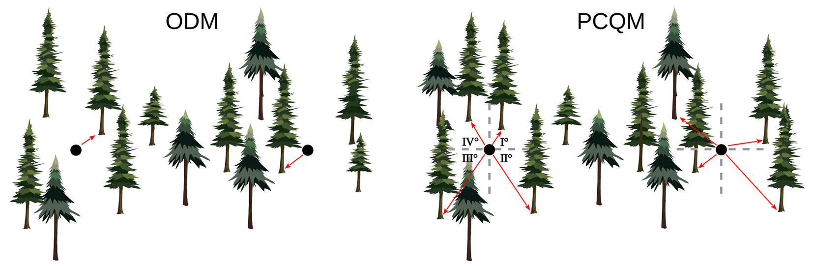
Among the plotless sampling methods, there are the ordered (or ranked) distance method (ODM - [27]) and the point-centred quarter method (PCQM) ([31]). The former involves measurement of the distance from the sampling point to the kth nearest tree, while the latter requires measurement of the distance from the sampling point to the kth nearest tree within sectors (usually quarters), in which the area around the point has been split (Fig. 1). The ODM was initially proposed by Moore ([26]) for density estimation based on distance from a sampling point to the nearest individual. Afterwards, it was extended by Morisita ([27]) to higher-order ranked distances (kth nearest individual). The PCQM, also known as the angle order method ([27]), was first employed in plant ecology by Cottam ([12]) and Cottam & Curtis ([13]), and later on formalized by Pollard ([31]). In practice the ODM appears more efficient than the PCQM, given that only one distance must be taken and it does not require locating sectors around the sampling point. Conversely, the PCQM is more time-intensive, requiring the measurement of four distances, locating more than four trees in the case of higher order distance (k > 1) and works well when it is easy to accurately partition the area around the sampling point into quarters.
Fig. 1 - Schematic representation of ODM and PCQM in field application.
The statistical bases of distance-based density estimators (DDEs) rely on the assumption that the target objects are distributed according to a homogeneous Poisson point process, which means that objects are randomly distributed and independent of each other ([11]). Unfortunately, real forests seldom satisfy this assumption ([19]) and the sensitivity of various DDEs to non-randomness distribution can yield biased results ([14], [11]). However, in non-random spatial patterns, and especially in clustered patterns, estimates from plot-based sampling methods (PSM) can also be biased ([5], [1], [29], [36]).
Despite the numerous studies conducted, the influence of the characteristics of density estimators, the underlying spatial pattern of the forest sampled, and the survey methodology, remain poorly understood in the performance of the DDEs ([11]). In addition, as far as we know, there are no published studies in which distance-based sampling methods have been applied in Italian forests to estimate stand attributes or have been tested as a potential alternative to the classic plot-based sampling. These considerations motivated us to assess the performance, in terms of accuracy and precision, of the ODM and PCQM in estimating the tree density and basal area, using data from real forest stands located in the Alpine area in northeastern Italy, by comparing the estimates with those obtained through a simulated plot-based sampling method.
Materials and methods
Study area
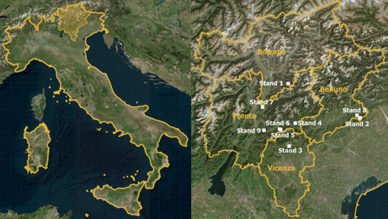
The forests considered in this study are located in the Alpine area of northeastern Italy (Fig. 2) where they are subjected to forest management practices. We selected 9 forest stands located on steep slopes at an elevation between 1000 and 1900 m a.s.l., mainly composed of Norway spruce (Picea abies Karst.), silver fir (Abies alba Mill.), beech (Fagus sylvatica L.), larch (Larix decidua Mill.) and Swiss stone pine (Pinus cembra L.). The main features of the forests selected are reported in Tab. 1.
Fig. 2 - Study area in northeastern Italy (left) and location of the forest stands (in white) in Bolzano, Belluno, Vicenza and Trento provinces (right). See Table 1 for details.
Tab. 1 - Main features of the selected forest stands (with the provinces in brackets) with corresponding R-index and associated spatial pattern. (a.s.l.): above sea level; (N): number of trees; (G): basal area; (Qmd): quadratic mean diameter); (*): The species composition is reported in decreasing values of abundance (Pa = Picea abies, Aa = Abies alba, Fs = Fagus sylvatica, Ld = Larix decidua, Pc = Pinus cembra, Ob = Other broad-leaved species, Oc = Other conifer species).
| Forest | Stand | Mean elevation (m a.s.l.) |
Tree species* | N (N ha-1) |
G (m2 ha-1) |
Qmd (cm) |
R-index | Spatial pattern |
|---|---|---|---|---|---|---|---|---|
| Latemar (Bolzano) | 1 | 1900 | Pa, Pc, Ld | 393 | 41.7 | 37 | 0.72 | Clustered |
| Cansiglio (Belluno) | 2 | 1400 | Pa, Fs, Aa | 790 | 45.2 | 27 | 0.80 | Clustered |
| Altopiano di Asiago (Vicenza) | 3 | 1000 | Pa, Aa | 1043 | 40.4 | 22 | 0.89 | Clustered |
| Tesino (Trento) | 4 | 1300 | Aa, Pa, Fs | 465 | 37.5 | 32 | 0.96 | Random |
| Val di Sella (Trento) | 5 | 1100 | Fs, Pa, Aa, Ld, Ob | 486 | 37 | 31 | 0.98 | Random |
| Val di Sella (Trento) | 6 | 1100 | Fs, Pa, Aa, Ld, Ob | 464 | 44.7 | 35 | 1.03 | Random |
| Val di Cembra (Trento) | 7 | 1200 | Fs, Pa, Ld, Aa, Ob, Oc | 549 | 47.1 | 33 | 1.08 | Regular |
| Cansiglio (Belluno) | 8 | 1400 | Pa, Fs, Aa | 951 | 54.9 | 27 | 1.15 | Regular |
| Altopiano della Vigolana (Trento) | 9 | 1100 | Aa, Ld, Ob | 522 | 39.1 | 31 | 1.19 | Regular |
Stand selection process
We collated geo-referenced data from field surveys previously conducted by academic and research institutions in the above-mentioned forests. As attributes of interest for this study, we considered the coordinates of trees and diameter at breast height.
From each forest, we identified and extracted 12 independent stands 1 ha wide (100 × 100 m), and classified each one according to its spatial pattern. In vegetation analysis, two main types of spatial patterns or dispersion, i.e., the arrangement of stationary objects on a plane ([15]), other than randomness, are known: regular (or uniform) and clustered (or aggregated). Clark & Evans ([9]) developed an index of aggregation (R-index) as a coarse measure of the spatial pattern, whose values range from 0 to 2.15. A value of R-index > 1 suggests regularity, an R-index < 1 suggests clustering, while an R-index = 1 suggests randomness. Thus, for each extracted stand, we calculated the R-index and performed a z-test for the significance against the null hypothesis of complete spatial randomness (i.e., uniform Poisson process). The package “spatstat” ([3]) in the R software environment ([32]) was used for the spatial point patterns analysis.
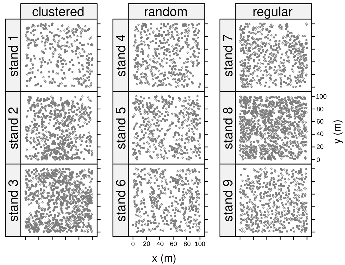
After computation of the R-index and classification of the stands, 9 stands were selected, encompassing the wider range of detected R-indices and representing the three main types of spatial patterns (Tab. 1, Fig. 3).
Fig. 3 - Spatial arrangement of trees of selected stands according to distribution patterns.
Plotless sampling survey
Within each stand, we simulated a plotless sampling survey by generating random sampling points under the condition of lying at least 6 m apart from the stand borders to avoid null quarters, especially when k > 1.
For the application of the PCQM, the distance from each sampling point to the 1st, 2nd and 3rd nearest tree in each of the quarters was calculated. For the application of the ODM, the minimum distance to the kth nearest tree within quarters was used.
For each method and distance to the kth tree, we used 10, 20 and 30 sampling points and the sampling was replicated 30 times. An initial amount of 900 random points was employed for 30 replicates, each of 30 sampling points. From the initial amount we randomly extracted 600 points for 30 replicates, each of 20 sampling points. Lastly, from the latter 600 points, we randomly extracted 300 points for 30 replicates, each of 10 sampling points.
Tree density estimation
In the ODM, over the distance measured from each random sampling point to the th nearest tree, e.g. the 1st or the 2nd or the 3rd, we applied the following formula for tree density estimation ([27], [31] - eqn. 1):
where λ is the estimated tree density, k the th nearest tree, n is the number of sampling points, π is the pi constant, and R2 is the square of the distance from the i-th random point to the k-th tree.
In the PCQM, first, the area around each random sampling point was partitioned into four equal-angular sectors (quarters) and then the distance to the th nearest tree, e.g., the 1st or the 2nd or the 3rd, was measured in each of the four quarters. After that, we applied the following formula for tree density estimation ([12], [31] - eqn. 2):
where λ is the estimated tree density, k is the th nearest tree, n is the number of sampling points, π is the pi constant, and R2 is the square of the distance from the ith random sampling point at the jth quarter to the kth tree.
Basal area estimation
Basal area was calculated using the diameter of trees for which the distance from the sampling point was measured. However basal area must be differently averaged, depending on whether ODM or PCQM is applied, as the ODM provides one diameter per sampling point, whereas the PCQM provides four diameters. The average basal area is then multiplied by tree density obtained from eqn. 1 in the case of ODM (eqn. 3), and by tree density obtained from eqn. 2 in the case of PCQM (eqn. 4):
where G is the basal area (m2 ha-1), n is the number of sampling points, π is the pi constant, dbh is the tree diameter (in cm) from the i-th random sampling point, at the j-th quarter for PCQM, λ1 and λ2 are the tree density derived from eqn. 1 and eqn. 2, respectively.
Accuracy and precision of estimates
We considered the accuracy, expressed in terms of relative error (RE), and the precision, expressed in terms of coefficient of variation (CV), as metrics to evaluate the estimates (i.e., tree density and basal area). Accuracy refers to the closeness of the estimate to the true value, whilst precision refers to the closeness of estimates to each other.
The accuracy and precision were computed as in the following formulas (eqn. 5, eqn. 6):
where σÌ‚ is the standard deviation of the estimated attribute. As a rule of thumb, the closer to zero both the accuracy and precision are, the better the estimates.
In addition, to evaluate whether the two plotless sampling methods could represent an alternative to PSM, we calculated the accuracy and precision of the tree density and basal area estimates obtained from a simulated plot-based sampling where the plots had different sizes. Since the plotless and plot-based sampling methods are conceptually different, it is impossible to establish equal conditions (i.e., the number of sampling points and area of a single sampling unit). Thus, we simulated plots with increasing area, i.e., 650, 1250, and 2500 m2, to compare the precision and accuracy of estimates with those obtained from plotless sampling methods with 10, 20 and 30 sampling points, respectively. The simulated PSM was replicated 30 times for each of the three plot-sizes.
Performance evaluation
We evaluated the overall performance of the two plotless sampling methods (m) by balancing the trade-off between accuracy and precision of the estimated attributes (i.e., tree density and basal area), within the several combinations of distance from the sampling point to the k-th nearest tree (k), the number of sampling points (nsp), as well as the spatial patterns (sp). With this aim, we employed the decision trees approach ([6]), a non-parametric partitioning technique which recursively performs univariate splits of the response variable (i.e., accuracy or precision) based on the values on a set of covariates (i.e., m, k, nsp, sp). Specifically, we used the conditional inference trees (CIT) which, differently from algorithms applying information measures such as the Gini coefficient, avoid overfitting and the selection bias towards covariates with many possible splits, by performing a significance test on the independence between covariates and response ([17]). In a CIT model, the hierarchical level of an inner node (i.e., the node having child nodes) is a qualitative measure of the importance of the embedded covariate, namely the closer the inner node to the root, the larger the importance of the embedded covariate. CIT models were implemented using the package “partykit” ([18]) in the R software environment.
Results and discussion
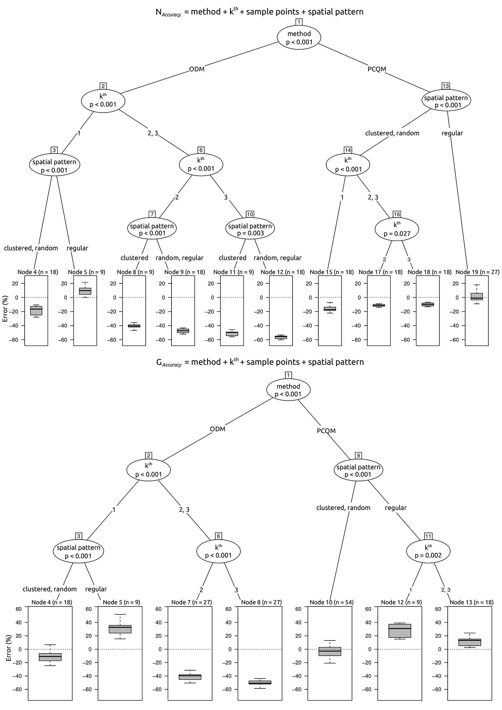
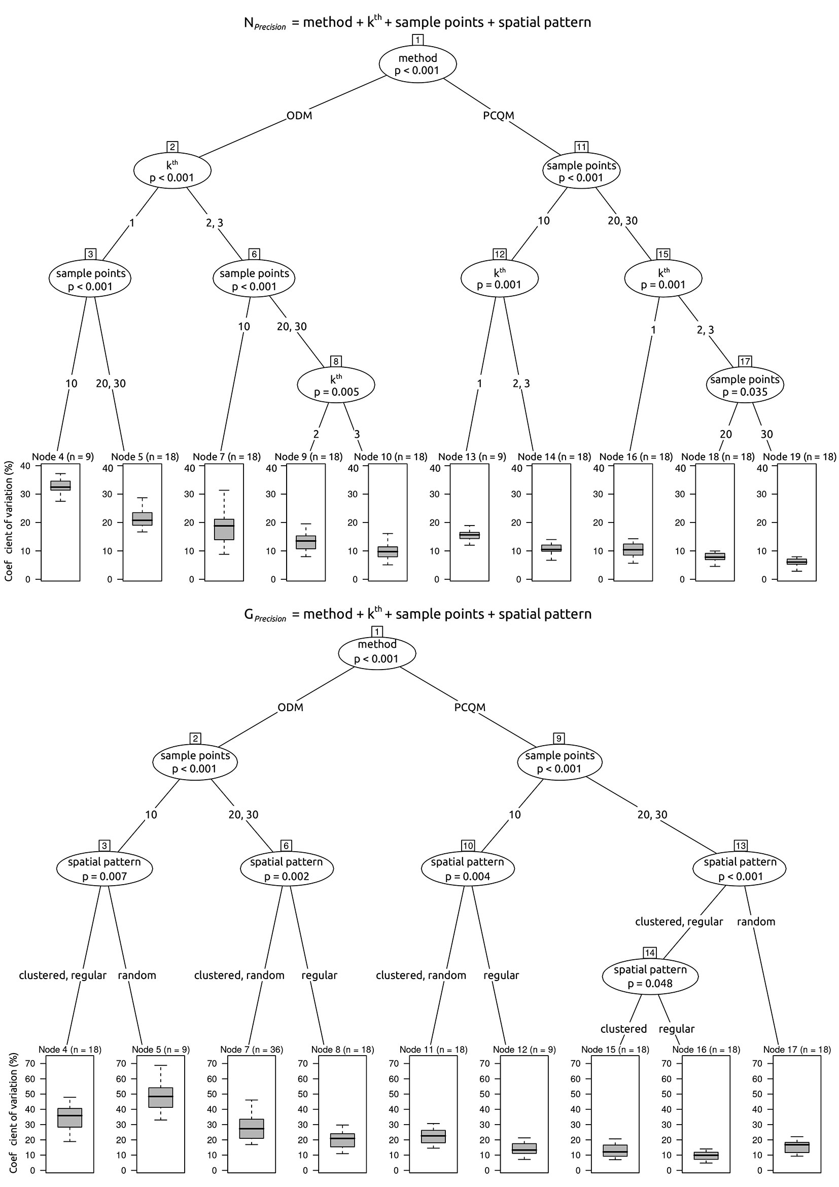
For the ODM the accuracy of estimates is primarily affected by the distance to the nearest tree and secondly by the spatial pattern (Fig. 4). The ODM provides unbiased and better accuracy of the estimates when k = 1, whatever the number of sampling points (Tab. 2, Tab. 3). Moreover, only when k is equal to 1, the accuracy of estimates provided by ODM does not differ from either the PCQM or PSM (Tab. 2, Tab. 3). The tree density estimate of ODM is more accurate in regular spatial patterns, whereas the basal area estimate is more accurate in clustered and random spatial patterns (Fig. 4). For k > 1, the accuracy of estimates of ODM strongly decreases (Tab. 2, Fig. 4). Regarding the precision, the estimate of tree density provided by the ODM is primarily affected by the distance to the nearest tree and, secondly, by the number of sampling points (Fig. 5). The precision of the tree density estimate provided by the ODM improves firstly at an increasing distance to the nearest tree and, secondly, at an increasing number of sampling points (Tab. 3, Fig. 5). Differently, the precision of the basal area estimate is less affected by the number of sampling points, although it improves with increasing the number of points. Lastly, the precision of estimates provided by ODM is significantly lower than PCQM whatever the attribute, distance to the nearest tree, and number of sampling points (Tab. 3). However, for the tree density estimate when k > 1, the precision of ODM does not differ from PSM (Tab. 2).
Fig. 4 - Accuracy (relative error) of estimates of tree density (above) and basal area (below).
Tab. 2 - Average values of accuracy (error) and precision (coefficient of variation) of the estimate of tree density, by distance to the kth nearest tree and number of sampling points, for the ODM, PCQM and PSM. Confidence intervals (95%) around the mean in square brackets. Values marked with an asterisk indicate the unbiased accuracy of estimates. In round brackets, the plot-size area is assumed to be comparable to the respective number of sampling points.
| k | # points | Accuracy (Error %) | Precision (Coefficient of variation %) | ||||
|---|---|---|---|---|---|---|---|
| ODM | PCQM | PSM | ODM | PCQM | PSM | ||
| 1 | 10 (650 m2) |
-9.10* [-19.80, 1.61] |
-7.60* [-16.50, 1.29] |
-7.37 [-12.20, -2.54] |
32.48 [30.39, 34.57] |
15.52 [14.24, 16.80] |
16.26 [12.89, 19.64] |
| 1 | 20 (1250 m2) |
-7.76* [-17.48, 1.96] |
-7.76* [-16.78, 1.25] |
-5.48* [-11.77, 0.81] |
23.05 [20.28, 25.82] |
10.71 [8.92, 12.50] |
11.49 [9.58, 13.39] |
| 1 | 30 (2500 m2) |
-8.62* [-18.08, 0.85] |
-7.74* [-16.57, 1.10] |
-4.32 [-8.52, -0.12] |
19.91 [18.65, 21.18] |
9.66 [8.30, 11.02] |
7.02 [5.15. 8.88] |
| 2 | 10 (650 m2) |
-46.59 [-49.54, -43.63] |
-7.92 [-12.27, -3.57] |
-7.37 [-12.20, -2.54] |
20.68 [16.88, 24.47] |
11.18 [9.70, 12.66] |
16.26 [12.89, 19.64] |
| 2 | 20 (1250 m2) |
-44.38 [-47.53, -41.22] |
-7.71 [-12.36, -3.05] |
-5.48* [-11.77, 0.81] |
14.83 [13.23, 16.44] |
8.11 [7.18, 9.05] |
11.49 [9.58, 13.39] |
| 2 | 30 (2500 m2) |
-44.28 [-46.80, -41.75] |
-7.93 [-12.54, -3.31] |
-4.32 [-8.52, -0.12] |
11.46 [10.03, 12.88] |
6.95 [5.80, 8.10] |
7.02 [5.15. 8.88] |
| 3 | 10 (650 m2) |
-55.95 [-58.21, -53.69] |
-7.13 [-10.32, -3.95] |
-7.37 [-12.20, -2.54] |
16.32 [13.45, 19.20] |
9.74 [8.07, 11.42] |
16.26 [12.89, 19.64] |
| 3 | 20 (1250 m2) |
-53.90 [-56.65, -51.15] |
-7.07 [-10.86, -3.29] |
-5.48* [-11.77, 0.81] |
11.36 [9.83, 12.89] |
7.15 [6.11, 8.20] |
11.49 [9.58, 13.39] |
| 3 | 30 (2500 m2) |
-53.76 [-56.09, -51.43] |
-7.41 [-10.99, -3.84] |
-4.32 [-8.52, -0.12] |
8.19 [6.78, 9.60] |
5.33 [4.49, 6.17] |
7.02 [5.15. 8.88] |
Tab. 3 - Average values of accuracy (error) and precision (coefficient of variation) of the estimate of basal area, by distance to the kth nearest tree and number of sampling points, for the ODM, PCQM and PSM. Confidence intervals (95%) around the mean in square brackets. Values marked with an asterisk indicate the unbiased accuracy of estimates. In round brackets, the plot-size area is assumed to be comparable to the respective number of sampling points.
| k | # points | Accuracy (Error %) | Precision (Coefficient of variation %) | ||||
|---|---|---|---|---|---|---|---|
| ODM | PCQM | PSM | ODM | PCQM | PSM | ||
| 1 | 10 (650 m2) |
5.02* [-12.10, 22.14] |
7.01* [-6.51, 20.53] |
-0.11* [-5.87, 5.65] |
45.70 [38.32, 53.08] |
21.65 [17.73, 25.58] |
20.32 [13.98, 26.65] |
| 1 | 20 (1250 m2) |
2.64* [-12.13, 17.41] |
4.88* [-6.96, 16.71] |
-1.13* [-4.69, 2.43] |
30.67 [25.85, 35.89] |
14.72 [11.55, 17.88] |
13.43 [9.32, 17.54] |
| 1 | 30 (2500 m2) |
2.97* [-11.10, 17.03] |
5.62* [-6.37, 17.61] |
0.27* [-3.51, 4.05] |
27.78 [24.86, 30.69] |
12.68 [10.22, 15.14] |
7.89 [5.90, 9.88] |
| 2 | 10 (650 m2) |
-43.03 [-47.01, -39.06] |
1.64* [-6.01, 9.28] |
-0.11* [-5.87, 5.65] |
37.20 [30.10, 44.30] |
19.64 [15.75, 23.53] |
20.32 [13.98, 26.65] |
| 2 | 20 (1250 m2) |
-39.97 [-42.51, -37.43] |
3.00* [-3.44, 9.45] |
-1.13* [-4.69, 2.43] |
28.61 [22.82, 34.40] |
14.02 [11.51, 16.53] |
13.43 [9.32, 17.54] |
| 2 | 30 (2500 m2) |
-40.18 [-43.35, -37.01] |
2.25* [-4.85, 9.34] |
0.27* [-3.51, 4.05] |
20.72 [17.33, 24.11] |
11.38 [9.02, 13.73] |
7.89 [5.90, 9.88] |
| 3 | 10 (650 m2) |
-52.13 [-56.23, -48.03] |
4.17* [-3.87, 12.20] |
-0.11* [-5.87, 5.65] |
35.83 [30.57, 41.08] |
17.88 [13.51, 22.25] |
20.32 [13.98, 26.65] |
| 3 | 20 (1250 m2) |
-50.00 [-53.02, -46.97] |
3.64* [-1.84, 9.12] |
-1.13* [-4.69, 2.43] |
24.50 [19.03, 29.97] |
12.95 [9.89, 16.00] |
13.43 [9.32, 17.54] |
| 3 | 30 (2500 m2) |
-50.21 [-53.23, -47.18] |
3.18* [-3.09, 9.45] |
0.27* [-3.51, 4.05] |
19.80 [15.47, 24.13] |
10.39 [7.16, 13.62] |
7.89 [5.90, 9.88] |
Fig. 5 - Precision (coefficient of variation) of estimates of tree density (above) and basal area (below).
The accuracy of estimates of PCQM is primarily affected by the spatial pattern and secondly by the distance to the nearest tree (Fig. 4). Averagely, the accuracy of the tree density estimate provided by PCQM is robust to both distance to the nearest tree and number of sampling points (Tab. 2). When k = 1 and in a regular spatial pattern, the PCQM provides an unbiased estimate of tree density (Tab. 2, Fig. 4). For basal area, the accuracy of the estimate provided by the PCQM is unbiased in clustered and random spatial patterns, regardless of distance to the nearest tree (Tab. 3, Fig. 4). In regular spatial patterns, PCQM provides a positively biased estimate of basal area, although the bias decreases when k > 1. The accuracy of estimates of PCQM does not differ from PSM and, in addition, it provides significantly better accuracy of estimates than the ODM when k > 1 (Tab. 2, Tab. 3).
The precision of estimates provided by the PCQM is primarily affected by the number of sampling points and, secondly, by the distance to the nearest tree, when the target attribute is tree density, or by the spatial pattern, when the target attribute is basal area (Fig. 5). The precision of estimates of PCQM is significantly better than the ODM and, at the same time, is comparable with PSM (Tab. 2, Tab. 3).
In our study, ODM provided satisfactory accuracy of estimates when k = 1 and an acceptable precision only for the tree density estimate when k > 1. To obtain the best results from ODM, Nielson et al. ([28]), after an extensive simulation study, suggested higher-order distance (i.e., k > 3) rather than a higher number of sampling points, when time and costs, along with field conditions, permit. Conversely, in our findings the accuracy of estimates of ODM strongly decreases when k > 1. This could be due to simulated populations which may exhibit lower local complexity in tree distribution patterns than the field-measured ones ([14]). In addition, we did not make trials for k > 3, as in field applications the larger the value of k the lower the advantage of plotless sampling methods against plot-based ones.
Differently from ODM, the PCQM provided overall satisfactory estimates, in terms of both accuracy and precision. However, according to Bryant et al. ([7]) and Cogbill et al. ([11]), but in disagreement with Jamali et al. ([19]), our results show biased estimates of the number of trees when k > 1. In opposition to other results ([27], [14], [28], [21]), in our study both plotless methods provided unbiased estimates of the number of trees in stands with regular spatial patterns and unbiased estimates of the basal area, in stands with clustered and random spatial patterns. It should be noted that the spatial pattern, elicited from the R-index calculated at stand scale (1 ha), can exhibit local departures within replicates, as in real forests stem distribution patterns may be non-stationary ([30]).
As pointed out by several authors ([31] [10]), the poorer performance of ODM, when compared to PCQM, is expected because density estimators based on a single distance (i.e., eqn. 1, eqn. 3) have generally larger variance than density estimators which average four distances (i.e., eqn. 2, eqn. 4), as for the PCQM. Furthermore, in our results, the plot-based estimates do not differ from those of PCQM, in terms of both accuracy and precision. Despite the higher field efforts required, due to the identification of the four equal-angular sectors, the PCQM proved to be the most effective method for a variety of forests ([2], [24], [21], [4], [19]).
It is known that the basic weakness of distance sampling methods relies on the assumption that the population to be sampled should be randomly scattered but, at the same time, complete spatial randomness is infrequently detectable in real forests ([31], [5]). Therefore, the effectiveness of a plotless density estimator must be evaluated considering its performance in non-random patterns and especially in clustered patterns, which are more frequent in real forests ([14]). Many studies confirmed the robustness of PCQM towards the bias related to non-random patterns ([14], [38], [22], [21], [4], [19]). Additionally, in our findings the PCQM provided estimates comparable to PSM. As a general rule, there is no unique plotless estimator for the accurate estimation of density for any spatial distribution pattern ([19]).
Conclusions
Distance-based sampling methods have long been proposed for forest surveys, however, to the best of our knowledge, they have never been applied to Italian forests, even for testing purposes. Although the small scale of this study cannot provide settled knowledge nor the generalization of findings, our results indicate that the plotless density estimators applied provide fairly accurate estimates of both tree density and basal area. Summing up, for the application of the ODM (i.e., the easier and faster option), achieving an accuracy and precision at most comparable to PSM, we recommend k=1 with at least 20 points (preferably 30); otherwise for the application of the PCQM (i.e., the time-consuming and laborious option), achieving an accuracy and precision better than PSM, we recommend k=2 even with 10 points (better with 20). Having to decide between the ODM and PCQM, all other things being equal, the latter is preferable.
We deem the evaluation of the distance-based density estimators through simulated plotless sampling surveys on real forest inventory datasets, encompassing different stand distribution patterns and densities, could offer an effective opportunity for revealing the main strength and weaknesses of plotless methods. The satisfactory results obtained, especially from PCQM, are encouraging for further trials over other Alpine as well as Apennine forests, and particularly on coppice stands which occupy almost the same area of the Italian high forests ([16]). If our results are confirmed, the plotless sampling methods (e.g., PCQM) could represent a valuable alternative whenever plot-based sampling is deemed redundant, or expensive in terms of cost and labour (e.g., assessment of the incidence of damages of storms, pests, animals, or spread of invasive alien species etc.), or when large-scale periodic monitoring must be conducted (e.g., EU Habitat Directive reporting). Lastly, the integration of a plotless sampling approach into an inventory framework at a regional, or sub-regional, scale could be an alternative to acquire more accurate estimates of key attributes concerning localized, and/or rare forest types which, by their nature, are not effectively detected at country scale by a national forest inventory.
Abbreviations
ODM: Ordered distance method; PCQM: Point-centred quarter method; PSM: plot-based sampling method; DDE: distance-based density estimator; CIT: conditional inference tree.
Acknowledgements
The authors gratefully thank Dr. Damiano Gianelle and Dr. Lorenzo Frizzera for the provision of data for the Val di Cembra forest used in this study.
References
Gscholar
Gscholar
Gscholar
Gscholar
Gscholar
Gscholar
Gscholar
Gscholar
Authors’ Info
Authors’ Affiliation
Nicola Puletti 0000-0002-2142-959X
Research centre for forestry and wood - Council for Agricultural Research and Economics - CREA, p.za Nicolini 6, I-38123 Trento (Italy)
Emanuele Lingua 0000-0001-9515-7657
Department of Land, Environment, Agriculture and Forestry - TESAF, University of Padua, v.le dell’Università 16, I-35020 Legnaro, PD (Italy)
Institute of BioEconomy, National Research Council of Italy, v. Biasi 75, I-38098 San Michele all’Adige, TN (Italy)
Corresponding author
Paper Info
Citation
Notarangelo M, Carrer M, Lingua E, Puletti N, Torresan C (2023). Performance assessment of two plotless sampling methods for density estimation applied to some Alpine forests of northeastern Italy. iForest 16: 385-391. - doi: 10.3832/ifor4335-016
Academic Editor
Mirko Di Febbraro
Paper history
Received: Feb 23, 2023
Accepted: Oct 25, 2023
First online: Dec 19, 2023
Publication Date: Dec 31, 2023
Publication Time: 1.83 months
Copyright Information
© SISEF - The Italian Society of Silviculture and Forest Ecology 2023
Open Access
This article is distributed under the terms of the Creative Commons Attribution-Non Commercial 4.0 International (https://creativecommons.org/licenses/by-nc/4.0/), which permits unrestricted use, distribution, and reproduction in any medium, provided you give appropriate credit to the original author(s) and the source, provide a link to the Creative Commons license, and indicate if changes were made.

Web Metrics
Breakdown by View Type
Article Usage
Total Article Views: 19850
(from publication date up to now)
Breakdown by View Type
HTML Page Views: 13799
Abstract Page Views: 2995
PDF Downloads: 2654
Citation/Reference Downloads: 5
XML Downloads: 397
Web Metrics
Days since publication: 919
Overall contacts: 19850
Avg. contacts per week: 151.20
Article Citations
Article citations are based on data periodically collected from the Clarivate Web of Science web site
(last update: Mar 2025)
Total number of cites (since 2023): 3
Average cites per year: 1.00
Publication Metrics
by Dimensions ©
Articles citing this article
List of the papers citing this article based on CrossRef Cited-by.
Related Contents
iForest Similar Articles
Research Articles
Advantages of the point-intercept method for assessing functional diversity in semi-arid areas
vol. 8, pp. 471-479 (online: 31 October 2014)
Research Articles
The effect of the calculation method, plot size, and stand density on the accuracy of top height estimation in Norway spruce stands
vol. 10, pp. 498-505 (online: 12 April 2017)
Research Articles
Application of machine learning models and Euclidean distance to predict soil spatial properties
vol. 19, pp. 186-194 (online: 02 June 2026)
Research Articles
Incorporating management history into forest growth modelling
vol. 4, pp. 212-217 (online: 03 November 2011)
Research Articles
Accuracy assessment of different photogrammetric software for processing data from low-cost UAV platforms in forest conditions
vol. 12, pp. 435-441 (online: 01 September 2019)
Research Articles
Evaluation of methods to improve the direct estimation of standing trees volume
vol. 18, pp. 87-92 (online: 17 April 2025)
Research Articles
Optimizing line-plot size for personal laser scanning: modeling distance-dependent tree detection probability along transects
vol. 17, pp. 269-276 (online: 07 September 2024)
Research Articles
Modelling diameter distribution of Tetraclinis articulata in Tunisia using normal and Weibull distributions with parameters depending on stand variables
vol. 9, pp. 702-709 (online: 17 May 2016)
Technical Advances
Forest stand height determination from low point density airborne laser scanning data in Roznava Forest enterprise zone (Slovakia)
vol. 6, pp. 48-54 (online: 21 January 2013)
Research Articles
Comparison of parametric and nonparametric methods for modeling height-diameter relationships
vol. 10, pp. 1-8 (online: 19 October 2016)
iForest Database Search
Google Scholar Search
Citing Articles
Search By Author
Search By Keywords


