Predicting total and component biomass of Chinese fir using a forecast combination method

doi:10.3832/ifor2243-010

Introduction

Forest biomass comprises the arboreal fraction of all existing plant mass in the forest, including stems, branches, leaves, and roots of forest trees ([19]). Due to its important role as carbon pool in forest ecosystems ([6]) and the laborious and costly process of measuring trees in the forest, there is a great demand to accurately predict tree biomass. A number of approaches for tree biomass prediction have been put forward. A widely used approach is the direct prediction of biomass using allometric relationships from tree measurements, such as diameter at breast height, total tree height, crown radius, and wood density ([4], [23], [7], [11]).

There are two methods for predicting total tree biomass with allometric equations: tree-level and component-level. The tree-level method involves a regression to predict total tree biomass. In the component-level method, prediction of total tree biomass is the sum of predictions of all tree components (leaves, branches, stem, and roots), obtained from separate regressions. There are strengths and weaknesses for each method. The tree-level biomass model predicts total tree biomass directly, but lacks detailed information on biomass of stems, branches, leaves, and roots. On the other hand, the component-level method provides more detailed information, but total tree biomass obtained by summing component predictions could often suffer from accumulation of errors and subsequently poor accuracy and precision. Moreover, in the component-level method, the sum of the biomass components can generate inconsistent results, as compared to predictions from the total biomass model ([16], [19]). To eliminate this inconsistency, several model estimation methods have been suggested to enforce additivity on a system of biomass equations ([8], [17], [20], [15], [3]).

Forecast combination, introduced by Bates & Granger ([1]), is a method to improve forecast accuracy ([14]). This method combines information generated from different models and distributes errors from these models, thus ensuring consistency of outputs from different models. Zhang et al. ([24]) used this method to combine tree-level and stand-level predictions of stand basal area.

The objective of this study was to evaluate current methods of predicting total and component biomass against the forecast combination method.

Materials and methods

Study sites

The plantations studied were at Weimin farm (Shaowu city, Fujian province) and Nianzhu farm (Fenyi city, Jiangxi province) in southern China (Fig. 1). Both sites belong to the subtropical monsoon climate region. In Weimin farm, mean annual precipitation is 1768 mm, mean annual temperature is 17.7 °C, and monthly mean temperature ranges from 6.8 °C in January to 28 °C in July. In Nianzhu farm, mean annual temperature and precipitation are 17.2 °C and 1656 mm, respectively.

Fig. 1 - Locations of the Chinese fir study sites in southern China.

Enlarge/Shrink Download Open In Viewer

Weimin farm consisted of stands of 7-, 16- and 28-year-old Chinese firs (Cunninghamia lanceolata [Lamb.] Hook.). Nianzhu farm consisted of stands of 28-year-old Chinese firs. One or two trees in each diameter class (2-cm) in each plot (0.06 ha) were randomly destructively sampled, totaling 39 sample trees in Weimin farm and 24 trees in Nianzhu farm (Tab. 1).

Tab. 1 - Mean and standard deviation (SD) for tree variables and component biomass of Chinese fir by location and age. Values in parentheses are ranges.

Location	Age	n	Stats	D (cm)	H (m)	Stem (kg)	Branch (kg)	Leaf (kg)	Root (kg)
Weimin	7	9	Mean	10.97 (5.7-16.3)	7.28 (4.9-9.3)	14.67	3.60	5.25	6.97
	7	9	SD	3.84	1.61	9.08	2.41	4.25	5.56
	16	14	Mean	14.19 (5.6-22.5)	11.48 (5.9-14.8)	34.26	2.63	3.45	11.38
	16	14	SD	5.28	2.70	22.57	2.50	3.18	8.90
	28	16	Mean	16.86 (8.7-27.8)	17.07 (10.3-22.7)	71.11	5.72	4.22	18.41
	28	16	SD	5.82	3.30	51.04	7.16	3.68	16.03
Nianzhu	28	24	Mean	18.70 (7.5-30.2)	16.89 (10.2-23.2)	86.67	6.82	4.65	21.26
Nianzhu	28	24	SD	7.13	3.57	64.90	6.97	4.53	18.18

Enlarge/Reduce Open in Viewer

Tree diameter at breast height (D) and height (H) was measured after the tree was felled. The fresh and dry weights of stem, branch, leaf and root were determined separately. From each stem, we sampled a 5-cm thick stem disc cut from the base of each 1-m stem segment, three subsamples of the branches and leaves from the upper, middle, and lower crown (1/3 of crown length, approximately 500-1000 g each), and samples (500-1000 g) from the stump, large structural roots (more than 10 mm), small roots (2-10 mm), and fine roots (less then 2 mm), obtained after excavation of the whole root system to the extent of the crown projection area. All samples were fresh weighted in the field, then transported to the laboratory where they were oven-dried to a constant weight at 105 °C and dry weighted. Dry weight was computed for each tree component by extrapolating the ratio of dry weight to fresh weight from subsamples.

Allometric equations

Standard allometric equations predict tree biomass as a power function of D ([11]). Other variables, such as total tree height, have also been proven to be important predictors ([4], [13]). The following two widely used equations ([12], [10], [23], [27], [21]) were considered in this study (eqn. 1, eqn. 2):

\begin{equation} M_{i} = a_{1}D_{i}^{b_{1}} + \varepsilon_{i} \end{equation}

\begin{equation} M_{i} = a_{2} (D_{i}^{2} H_{i})^{b_{2}} + \varepsilon_{i} \end{equation}

where M_i is the biomass (kg) for the i-th tree, a and b are the regression parameters to be estimated, D_i is the tree diameter (cm), H_i is the total height (m), and ε_i is the random error.

The separate model method involves employing separate regression models to predict total tree biomass and its components: branch, leaf, root, and stem. Based on a preliminary analysis, we found that the eqn. 1 performed better than eqn. 2 on modeling branch, leaf and root biomass. However, in terms of the stem and total biomass, the eqn. 2 was better than eqn. 1. Thus, the following equation forms were selected (eqn. 3 to eqn. 7):

\begin{equation} \text{Branch}: M_{Bi} = a_{3B} D_{i}^{b_{3B}} + \varepsilon_{i} \end{equation}

\begin{equation} \text{Leaf}: M _{Li} = a _{4L} D _{i} ^{b _{4L} } + \varepsilon_{i} \end{equation}

\begin{equation} \text{Root}: M _{Ri} = a _{5R} D _{i} ^{b _{5R} } + \varepsilon_{i} \end{equation}

\begin{equation} \text{Stem}: M _{Si} = a _{6S} (D _{i} ^{2} H_{i})^{b _{6S} } + \varepsilon_{i} \end{equation}

\begin{equation} \text{Total}: M _{Ti} = a _{7T} (D _{i} ^{2} H _{i} )^{b _{7T} } + \varepsilon_{i} \end{equation}

where all variables are as defined earlier, with added subscripts to denote component types.

The models were separate in the sense that prediction of total tree biomass from eqn. 7 did not equal the sum of predictions for components from eqn. 3 to 6. In other words, the equations were not constrained to be additive. Parameters of eqn. 3 to 7 were simultaneously obtained by using Seemingly Unrelated Regression (SUR). SAS procedure MODEL ([18]) was used for this purpose.

The Additive model approach was based on the procedure developed by Parresol ([15]). The following system of equations was used to predict total tree biomass and its components (eqn. 8 to eqn. 12):

\begin{equation} \text{Branch}: M_{Bi} = a_{8B} D_{i}^{b_{8B}} + \varepsilon_{i} \end{equation}

\begin{equation} \text{Leaf}: M_{Li} = a_{9L} D_{i}^{b_{9L}} + \varepsilon_{i} \end{equation}

\begin{equation} \text{Root}: M_{Ri} = a_{10R} D_{i}^{b_{10R}} + \varepsilon_{i} \end{equation}

\begin{equation} \text{Stem}: M _{Si} = a _{11S} (D _{i} ^{2} H_{i})^{b _{11S} } + \varepsilon_{i} \end{equation}

\begin{equation} \text{Total}: M_{TSI} = \hat{M}_{Bi} + \hat{M} _{Li} + \hat{M} _{Ri} + \hat{M} _{Si} + \varepsilon_{i} \end{equation}

where the symbol ^ on top of a variable name denotes the predicted value for that variable.

Eqn. 8 to 11 have the same forms as eqn. 3 to 6, respectively. Prediction of total tree biomass (eqn. 12) was obtained by summing predictions of component biomass. Again, SUR was used to estimate parameters of this system of equations.

Zhang et al. ([24], [25]) applied the forecast combination method to combine different types of models for predicting stand basal area and stand survival. A similar approach was applied in this study to predict total tree biomass by combining: (a) direct prediction from the regression model (eqn. 7); and (b) indirect prediction by summing predictions from component models (eqn. 13):

\begin{equation} \hat{M}_{Fi} = w_{1} M_{Ti} + w_{2} M_{TSi} \end{equation}

where {hat} M_Fi is the prediction of total tree biomass from forecast combination, w₁ and w₂, are weights, with w₁ + w₂ = 1, {hat}M_Ti is the direct prediction of total tree biomass from eqn. 7, and {hat} M_TSi is the indirect prediction of total tree biomass by summing predictions from component biomass equations. Depending on the component biomass equations, two methods of Forecast Combination were considered in this study: (i) FC1 that used the sum of predictions from the Separate model (eqn. 3-6); and (ii) FC2 that used the sum of predictions from the Additive model (eqn. 12). The weight coefficients of the combined tree biomass model could be obtained by the optimal weight method ([24] - eqn. 14):

\begin{equation} W = {\frac{ E^{-1} R} {R^{T} E^{-1} R }} \end{equation}

where (eqn. 15 to eqn. 18):

\begin{equation} W = (w_{1}, w_{2})^{T} \end{equation}

\begin{equation} R = (1, 1)^{T} \end{equation}

\begin{equation} E = \left (\array{ e_{1}^{T} e_{1} & e _{1} ^{T} e _{2} \\ e _{2} ^{T} e _{1} & e _{2} ^{T} e _{2}} \right) \end{equation}

\begin{equation} e_{k} = ( \varepsilon_ {k1}, \varepsilon _{k2},\ldots, \varepsilon _{kn} ) \end{equation}

where ε_ki is the prediction error for the tree i using the method k, with k = 1, 2, and i = 1, 2, …, m, being m the total number of trees; T is the transport matrix.

The component predictions were then adjusted to add up to the combined estimator for total tree biomass. This was accomplished by multiplying the component predictions by λ, the adjusting coefficient, which is calculated as (eqn. 19):

\begin{equation} \lambda = \hat{M}_{Fi} / \hat{M}_{TSi} \end{equation}

In this study, the two-fold leave-one-out cross validation scheme was used for model validation. First, the models were fitted using data from the Weimin farm, and then validated using data from the Nianzhu farm. Second, we treated Nianzhu data as the fit data and Weimin data the validation data. Evaluation statistics were computed based on observations pooled from the two validation data sets. The evaluation statistics of mean difference (MD), mean absolute difference (MAD), and R² ([24]) were used to validate the models. Models with lower MD and MAD values indicate a better fit to the data.

Results and discussion

The stem biomass ranged from 14.67 to 86.67 kg, branches from 2.63 to 6.82 kg, leaves from 3.45 to 5.25 kg, and roots from 6.77 to 21.23 kg (Tab. 1). Stem biomass accounted for more than 50% of the total tree biomass, except the stand of age 7, which could explain the same equation (eqn. 2) of stem and total tree biomass in the preliminary analysis. The parameter estimates and their standard deviation errors were slightly different between the Separate model and Additive models in the Weimin and Nianzhu farms (Tab. 2), being their values more consistent across methods than across farms. For total tree biomass prediction, the MD value obtained using the FC1 method (the Forecast Combination method that used separate models) was 83.46% smaller than that obtained using the additive model and 41.04% smaller than that of the FC2 method (Forecast Combination method that used additive model). Moreover, the FC1 method produced the best R² values, while the Separate model method yielded the lowest MAD value (Tab. 3). Regarding the prediction of component biomass, the FC1 method had the best MAD and R² values for all components (except leaf biomass) and the best MD values for two of the four components (Tab. 4).

Tab. 2 - Parameter estimates and standard errors (SE) of the biomass model using Separate and Additive models in the Weimin and Nianzhu farms.

Parameter	Weimin		Nianzhu
Parameter	Estimates	SE	Estimates	SE
a _3B	8.2e-5	6.4e-5	8.84e-4	0.0013
b _3B	3.7571	0.2425	2.9377	0.4520
a _4L	0.0276	0.0215	0.0009	0.0013
b _4L	1.7984	0.2574	2.7953	0.4455
a _5R	0.0110	0.0047	0.0200	0.0103
b _5R	2.5401	0.1383	2.3165	0.2503
a _6S	0.0247	0.0053	0.0397	0.0131
b _6S	0.9141	0.0236	0.8647	0.0346
a _7T	0.0337	0.0066	0.0435	0.0156
b _7T	0.9211	0.0215	0.8897	0.0376
a _8B	0.0001	8.6e-5	0.0015	0.0021
b _8B	3.7089	0.2966	2.7895	0.4583
a _9L	0.0432	0.0396	0.0010	0.0015
b _9L	1.6763	0.3055	2.7802	0.4539
a _10R	0.0089	0.0041	0.0114	0.0058
b _10R	2.6206	0.1480	2.4950	0.2641
a _11S	0.0224	0.0049	0.0369	0.0121
b _11S	0.9254	0.0239	0.8726	0.0344

Enlarge/Reduce Open in Viewer

Tab. 3 - Evaluation statistics for total tree biomass prediction by method. (§): denotes the best method based on each fitting statistic (MD, MAD, R²).

Method	MD	MAD	R²
Separate model	0.5761	8.0296^(§)	0.9772
Additive model	-0.7199	8.6210	0.9726
Combined using Separate model	0.1191^(§)	8.0469	0.9780^(§)
Combined using Additive model	0.2020	8.0802	0.9776

Enlarge/Reduce Open in Viewer

Tab. 4 - Evaluation statistics for component biomass prediction by method. (§): denotes the best method based on each fitting statistic (MD, MAD, R²).

Component	Method	MD	MAD	R²
Branch	Separate model	-0.1511	1.9476	0.6601
	Additive model	-0.487	2.0743	0.6371
	Combined using Separate model	-0.0853^(§)	1.9307^(§)	0.6786^(§)
	Combined using Additive model	-0.3997	2.0213	0.6755
Leaf	Separate model	0.7034^(§)	2.0181^(§)	0.4952^(§)
	Additive model	0.4883	2.0838	0.4424
	Combined using Separate model	0.7343	2.0768	0.4332
	Combined using Additive model	0.5259	2.1002	0.4311
Root	Separate model	-0.2353	3.2619	0.8807
	Additive model	-0.2625	3.3982	0.8686
	Combined using Separate model	-0.0046^(§)	3.2564^(§)	0.8905^(§)
	Combined using Additive model	-0.0466	3.2853	0.8872
Stem	Separate model	-0.298	4.7543	0.9832
	Additive model	-0.4586	4.9985	0.9831
	Combined using Separate model	0.1986	4.2931^(§)	0.9865^(§)
	Combined using Additive model	0.1224^(§)	4.5509	0.9851

Enlarge/Reduce Open in Viewer

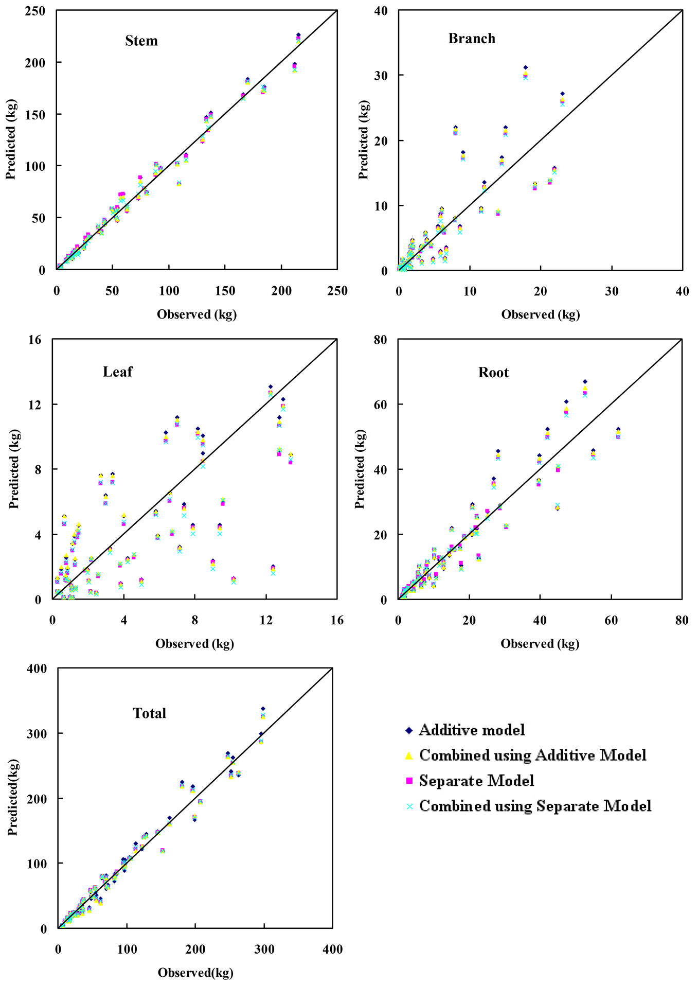
Fig. 2 displays the predicted vs. observed biomass of total and component biomass. Most of biomass predictions were distributed near the straight line (y=x) using any of the four methods used (Fig. 2). It can be noticed that the predictions of leaf biomass showed the lowest accuracy and precision among all the component biomass.

Fig. 2 - Observed vs. predicted total and component biomass by each method.

Enlarge/Shrink Download Open In Viewer

Additive vs. separate model

Parameters of the component regression models in the Additive model approach were subjected to the constraint that the sum of component predictions from the resulting models would be equal to the total biomass ([9], [3], [5]). On the other hand, the Separate model method did not involve any constraints, thus its parameters resulted 19.97% and 6.86% lower for MD, MAD, respectively and 0.47% larger for R² than those of the Additive model method used for modeling total tree biomass (Tab. 3). Furthermore, the separate model method produced the best MD, MAD and R² values for all components. The sole exception using the latter method was leaf biomass, which showed a lower MD value (Tab. 4). However, due to lack of additivity constraint, the sum of predictions from different biomass components was not equal to the prediction of total tree biomass in the Separate model approach ([19]). Therefore, the advantage of a compatible, additive system for total and component biomass in the Additive model method was also accompanied by a decrease in the accuracy and precision of predictions.

Forecast combination

This approach involves a combined estimator, which is the weighted average of the predictions from the total biomass equation and the sum of predictions of component biomass from either (a) the separate model, or (b) the additive model. Yue et al. ([22]) used the variance-covariance method to calculate weight coefficients for the combined model. Zhang et al. ([26]) reported that the optimal weight method (i.e., the ordinary least squares estimate of the weights) performed better than the variance-covariance method. Here, the optimal weight method was used to calculate weight coefficients of combined model of tree biomass. Compared to the method using the additive model (FC2), the Forecast Combination method that used the separate model (FC1) gave better values of MD, MAD, and R² for total and component biomass prediction (Tab. 3, Tab. 4). The only exceptions were MD values for leaf and stem biomass. The sum of component predictions from the Separate model was not subject to any constraint, and therefore could be different from the prediction from the total biomass equation. The combined predictions of FC1 method benefit from non-constraint of the Separate model, thus increasing the accuracy and precision as compared to the FC2 estimation.

Forecast combination vs. additive model

Tree biomass additivity has long been recognized as a desirable property of biomass estimation. Several studies have successfully solved the logical inconsistency between the components and total tree predictions ([17]) by developing a system of additive biomass equations estimated by the SUR method, thus providing a statistically correlated system of equations with restrictions ([15], [2]). In this study, a forecast combination with adjusted coefficient (a consistent value) was applied, ensuring the additivity of the component biomass. It is worth noting that the adjusted coefficient may vary across the biomass components, because the ratio between each component depends on site quality, stand density, age or tree size.

The FC1 method outperformed the Additive model method in predicting the total tree biomass, based on all three evaluation statistics. The FC1 method also produced better values of MD, MAD, and R² for predicting branch, root, and stem biomass. For leaf biomass, the FC1 method resulted in better MAD, but worse MD and R² values, as compared to the Additive model method (Tab. 3, Tab. 4).

Forecast combination vs. separate model

In the Separate model method, the prediction of total tree biomass for each tree is directly derived from the total biomass regression equation. The FC1 method combined the information from this prediction and the sum of predictions from regression equations for each component biomass. The result is an improvement of two (MD and R²) out of three fitting statistics for total tree biomass predictions obtained using the FC1 method, as compared with the Separate model method (Tab. 3). Indeed, the MD value derived from FC1 method was 79.33% smaller than that obtained using the Separate model method, while the R² value from FC1 method was slightly larger than that of the Separate model method.

For the component biomass, predictions from the Separate model method were unadjusted predictions from the regression models. These predictions were then adjusted such that the resulting sum matched the combined estimator for total biomass in the FC1 method.

Based on all three evaluation statistics, the FC1 method showed better performances in predicting branch, root, and stem biomass as compared to the Separate model, whereas the latter method yielded more accurate predictions of leaf biomass. The opposite trend observed in leaf biomass predictions might be due to low R² values of separate leaf biomass model (Tab. 4). In the forecast combination method, the implicit assumption was that the relationship between observed and predicted values from different models was stable. If this relationship remains relatively unchanged from the sample data to the population, then the combined value should provide better predictions than those by any model alone ([26]). However, in this study the relationship in leaf biomass was not stable, as inferred from R² values ranging from 0.43 to 0.49 (Tab. 4).

Conclusions

The Forecast Combination method takes advantages of information from tree-level and component-level models, by providing an estimator that combines predictions from these models. To ensure additivity, component predictions from the Separate model were adjusted to match the combined estimator for total tree biomass. This approach was superior to the Additive model method in predicting total tree biomass and all of its components, except for leaf biomass.

Acknowledgments

The authors gratefully acknowledge the Fundamental Research Funds for the Central Non-profit Research Institution of CAF (CAFYBB2017ZX001-2), the National Natural Science Foundation of China (No. 31670634), and the Scientific and Technological Task in China (No. 2016YFD0600302-1).

References

(1)

Bates JM, Granger CWJ (1969). The combination of forecasts. Operational Research Society 20 (4): 451-468.
::CrossRef::Google Scholar::

(2)

Bi H, Long Y, Turner J, Lei Y, Snowdon P, Li Y, Harper R, Zerihun A, Ximenes F (2010). Additive prediction of aboveground biomass for Pinus radiata (D. Don) plantations. Forest Ecology and Management 259 (12): 2301-2314.
::CrossRef::Google Scholar::

(3)

Bi H, Turner J, Lambert MJ (2004). Additive biomass equations for native eucalypt forest trees of temperate Australia. Trees 18: 467-479.
::CrossRef::Google Scholar::

(4)

Chave J, Andalo C, Brown S, Cairns MA, Chambers JQ, Eamus D (2005). Tree allometry and improved estimation of carbon stocks and balance in tropical forests. Oecologia 145 (1): 87-99.
::CrossRef::Google Scholar::

(5)

Dong L, Zhang L, Li F (2014). A compatible system of biomass equations for three conifer species in Northeast, China. Forest Ecology and Management 329: 306-317.
::CrossRef::Google Scholar::

(6)

Fahey TJ, Woodbury PB, Battles JJ, Goodale CL, Hamburg SP, Ollinger SV, Woodall CW (2010). Forest carbon storage: ecology, management, and policy. Frontiers in Ecology and the Environment 8: 245-252.
::CrossRef::Google Scholar::

(7)

Goodman RC, Phillips OL, Baker TR (2014). The importance of crown dimensions to improve tropical tree biomass estimates. Ecological Applications 24: 680-698.
::CrossRef::Google Scholar::

(8)

Jacobs MW, Cunia T (1980). Use of dummy variables to harmonize tree biomass tables. Canadian Journal of Forest Research 10: 483-490.
::CrossRef::Google Scholar::

(9)

Kozak A (1970). Methods for ensuring additivity of biomass components by regression analysis. Forestry Chronicle 46: 402-404.
::CrossRef::Google Scholar::

(10)

Lambert MC, Ung CH, Raulier F (2005). Canadian national tree aboveground biomass equations. Canadian Journal of Forest Research 35 (8): 1996-2018.
::CrossRef::Google Scholar::

(11)

MacFarlane DW (2015). A generalized tree component biomass model derived from principles of variable allometry. Forest Ecology and Management 354: 43-55.
::CrossRef::Google Scholar::

(12)

Medhurst JL, Battaglia M, Cherry ML, Hunt MA, White DA, Beadle CL (1999). Allometric relationships for Eucalyptus nitens (Deane and Maiden) Maiden plantations. Trees 14: 91-101.
::CrossRef::Google Scholar::

(13)

Molto Q, Hérault B, Boreux JJ, Daullet M, Rousteau A, Rossi V (2013). Predicting tree heights for biomass esitmates in tropical forests. Biogeosciences Discuss 10: 8611-8635.
::CrossRef::Google Scholar::

(14)

Newbold P, Zumwalt JK, Kannan S (1987). Combining forecasts to improve earnings per share prediction and examination of electric utilities. International Journal of Forecasting 3 (2): 229-238.
::CrossRef::Google Scholar::

(15)

Parresol BR (2001). Additivity of nonlinear biomass equations. Canadian Journal of Forest Research 31: 865-878.
::CrossRef::Google Scholar::

(16)

Parresol BR (1999). Assessing tree and stand biomass: a review with examples and critical comparisons. Forest Science 45: 573-593.
::Online::Google Scholar::

(17)

Reed D, Green EJ (1985). A method of forcing additivity of biomass tables when using nonlinear models. Canadian Journal of Forest Research 15: 1184-1187.
::CrossRef::Google Scholar::

(18)

SAS Institute Inc (2009). SAS/ETS 9.2 user’s guide. SAS Publishing, Cary, NC, USA, pp. 2908.
::Google Scholar::

(19)

Sanquetta CR, Behling AB, Corte APD, Netto SP, Schikowski AB, Do Amaral M (2015). Simultaneous estimation as alternative to independent modeling of tree biomass. Annals of Forest Science 72: 1099-1112.
::CrossRef::Google Scholar::

(20)

Tang S, Zhang H, Xu H (2000). Study on establish and estimate method of compatible biomass model. Scientia Silvae Sinicae 36 (1): 19-27. [in Chinese with English abstract]
::Google Scholar::

(21)

Tang X, Lu Y, Fehrmann L, Forrester DI, Guisasola-Rodíguez R, Pérez-Cruzado C, Kleinn C (2016). Estimation of stand-level aboveground biomass dynamics using tree ring analysis in a Chinese fir plantation in Shitai County, Anhui Province, China. New Forests 47: 319-332.
::CrossRef::Google Scholar::

(22)

Yue C, Kohnle U, Hein S (2008). Combining tree-and stand-level models: a new approach to growth prediction. Forest Science 54 (5): 553-566.
::Online::Google Scholar::

(23)

Zhang X, Duan A, Zhang J (2013). Tree biomass estimation of Chinese fir (Cunninghamia lanceolata) based on Bayesian method. PLoS ONE 8 (11): e79868.
::CrossRef::Google Scholar::

(24)

Zhang X, Lei Y, Cao QV (2010). Compatibility of stand basal area predictions based on forecast combination. Forest Science 56: 552-557.
::Online::Google Scholar::

(25)

Zhang X, Lei Y, Cao QV, Chen X, Liu X (2011a). Improving tree survival prediction with forecast combination and disaggregation. Canadian Journal of Forest Research 41: 1928-1935.
::CrossRef::Google Scholar::

(26)

Zhang X, Lei Y, Chen X (2011b). Comparison of weight computation in stand basal area combined model. Scientia Silvae Sinicae 47 (7): 36-41. [in Chinese with English abstract]
::Online::Google Scholar::

(27)

Zhao D, Kane M, Michael D, Teskey R, Clutter M (2015). Additive tree biomass equations for midrotation loblolly pine plantations. Forest Science 61: 613-623.
::CrossRef::Google Scholar::

Previous Next Close

Predicting total and component biomass of Chinese fir using a forecast combination method Zhang et al. (2017). iForest 10: 687-691. - doi: 10.3832/ifor2243-010