Feasibility study of near infrared spectroscopy to detect yellow stain on cork granulate
iForest - Biogeosciences and Forestry, Volume 11, Issue 1, Pages 111-117 (2018)
doi: https://doi.org/10.3832/ifor2563-010
Published: Jan 31, 2018 - Copyright © 2018 SISEF
Research Articles
Collection/Special Issue: INCOTW - Sassari, Italy (2017)
International Congress on Cork Oak Trees and Woodlands
Guest Editors: Piermaria Corona, Sandro Dettori
Abstract
The aim of this study was to evaluate the viability of near infrared spectroscopy (NIRS) to detect the anomaly known as yellow stain on cork granulate. Detecting this anomaly is crucial to the cork granulate stopper industry, since it is associated with the presence of 2.4.6-Trichloroanisole (TCA), this compound having been identified as the main agent responsible for cork off-flavours. Samples for the NIRS spectra were prepared by mixing in different proportions cork granulate with high visual quality and cork granulate with yellow stain, obtaining 120 samples with 8 different percentages of yellow stain (0, 5, 10, 15, 25, 35, 50 and 100%). Two spectra per sample were collected using a Bruker MPA spectrophotometer and the partial least squares (PLS) method was used to obtain numerous equations. The best equation was obtained by utilizing the standard normal variate (SNV) spectral preprocessing, making use of only one specific part of the near infrared spectral range: 9400-4250 cm-1. This equation shows a coefficient of determination (R²) of 99.42%, a root mean square error of cross validation (RMSECV) of 2.34%, and a residual prediction deviation (RPD) of 13.10. The critical level and the limit of detection are 3.8% and 7.6%, respectively. The calculated receiver operating characteristic (ROC) curves show great discrimination capacity and the area under the ROC curve (AUC) is higher than 0.93 in any case. This study demonstrates that NIRS provides a viable technique for detecting yellow stain in cork granulate.
Keywords
Cork, Granulate, Yellow Stain, 2.4.6-Trichloroanisole, TCA, Near Infrared Spectroscopy, NIRS
Introduction
Cork is obtained from the cork oak tree (Quercus suber L.) through successive harvests at given time intervals without the need to cut down the trees, and it is therefore considered a sustainable product. Although cork forests are found in Algeria, France, Italy, Morocco, Portugal, Spain and Tunisia ([26]), most of them are concentrated in Portugal (34%) and Spain (27%), followed by Morocco with 18% ([1]). Cork from the Iberian Peninsula accounts for about 80% of the raw cork extracted yearly, 49.6% of that corresponds to Portugal and 30.5% to Spain ([1]). Cork has numerous applications though the most important of these in economic terms is the manufacture of different types of cork stoppers to be used in the bottling of wines ([25]). It is the suitability of the raw cork material for this production that establishes its commercial value ([16]). Agglomerated, micro-agglomerated and technical stoppers are made from cork granulate which is obtained by grinding the cork that is not suitable for the production of natural cork stoppers and disks, as well as from the waste generated during cork manufacturing ([24]). Cork granulate is defined as cork fragments between 0.2 and 8.0 mm in size ([31]) and represents an important part of the cork industry, accounting for 75% of total cork ([9]).
One of the main problems for the cork industry is the presence of 2,4,6-Trichloroanisole (TCA - [2]). This compound has been identified as the main agent responsible for cork off-flavours ([6], [29]) and is formed through fungal degradation of the chlorophenols present in the cork. Various studies have attributed this phenomenon to different species of fungi such as Penicillium and Aspergillus ([5]) or Armillaria ([22]). TCA has mould-like taste that will be present in the wine ([23]) and it also has a very low detection threshold, 1.4-4 ng l-1 ([8]). Attenuated total reflection infrared spectroscopy (ATR-IR) proved that the presence of TCA modifies the cork spectra ([8]). In this regard, two new bands appeared at 1417 and 1314 cm-1 and the relative intensities of the bands increased at 1039 and 813 cm-1 ([8]). At present, TCA control is only being developed for cork stoppers, using chromatographic ([11]) or sensory techniques ([12]) and research is ongoing in this area ([27], [28]). However, these techniques cannot be applied to raw material (planks or granulate) for 2 reasons, namely, the high cost and high variability of the material.
The cork defect known as “yellow stain” was identified as far back as 1900 ([4]). Studies performed using scanning electron microscopy (SEM) carried out on healthy cork and cork with yellow stain showed that the cellular structures of the infected and the healthy tissues were different, and that the tissues attacked were composed of deformed, wrinkly cells with cell wall separation at the middle lamella level ([22]). These changes were related to the degradation of lignin and pectin, as evidenced by the deposition of calcium in the intercellular space of the cells attacked ([22]). Comparative chemical studies showed that the cork attacked by yellow stain suffered a degradation of tannins with consequent discoloration ([7]) along with a biosynthesis of TCA ([15]).
Hence, the industry would greatly benefit from the development of a method to control the presence of yellow stain in cork granulate. If cork granulate affected by yellow stain and therefore by TCA is not removed from the production line, the granulate cork stoppers produced using this defective material will have a mould-like taste and therefore will not be suitable for wine bottle closure. Near infrared spectroscopy (NIRS) is potentially suitable for detecting yellow stain in cork granulate, since it is widely used in quality control of granulated products in the food and agriculture industry ([14], [17]). In addition, NIRS has certain advantages over other analytical methods, such as rapid and non-destructive analysis, low analyzing costs and easy sample preparation. Furthermore, it can also provide information on different variables simultaneously.
The first application of NIRS technology to cork was a viability study to assess its potential for characterizing cork planks according to visual quality, porosity and moisture content, and for predicting the geographical origin of cork planks ([18]). The potential of this technology as a method for predicting the geographical origin of cork planks and stoppers has been demonstrated ([19]). It allows continuous quality control of moisture content in cork stoppers while simultaneously obtaining other parameters such as chemical components (waxes and total polyphenols) along with physical and mechanical parameters (density, extraction force and compression force) ([20]). It is useful for determining the porosity of cork planks before and after boiling ([25]). The last application of this technology is the development of NIRS models to predict the technological parameters (caliper, earthy cork, blown cork, belly and stained cork) on cork planks ([21]).
The aim of this study is to develop calibration equations to predict the percentages of yellow stain in samples of cork granulate and thereby evaluate the viability of NIRS as a method to detect cork with yellow stain on the production line. Numerous spectra preprocessing and spectral ranges were studied to determine the most suitable. Lastly, critical level, limit of detection and receiver operating characteristic (ROC) curves of the equations were also studied.
Material and methods
Samples and sample preparation
Cork pieces used in this study were collected in a sampling carried out in Catalonia (Spain) in 1991 and form part of the INIA-CIFOR cork laboratory collection. Two groups were selected: pieces classified as being of the highest visual quality (HQ - Fig. 1a), completely free of defects, and pieces where yellow stain was clearly present (YS - Fig. 1b).
Fig. 1 - (a) Piece of cork classified as highest visual quality (HQ); (b) piece of cork with yellow stain clearly present (YS).
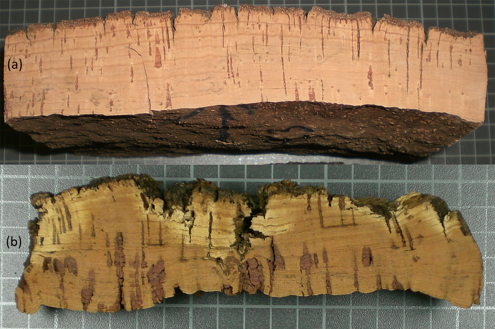
Five strips of 0.5 cm thickness were cut from the cross section on all the pieces from both groups and the corkback (phloemic tissue remaining on the outer side of the cork) was removed. In the case of YS pieces, areas presenting yellow stain were separated, so that areas of “pure cork” and “stained cork” were separately ground and sieved (0.5-1 mm) in order to obtain cork granulate of two types: one comprising 100% highest visual quality cork with no defects ,and the other, 100% yellow stained cork. Both types of cork granulate were dried at 103 °C to constant weight and later conditioned in a container at constant temperature. When the samples were scanned, average moisture content was 4.5%.
Samples for the NIRS spectra were prepared by mixing both types of cork granulate in different proportions, obtaining samples with different percentages of yellow stain (YSP). These percentages were established such that the range was as large as possible while at the same time having a greater incidence of lower values: 0, 5, 10, 15, 25, 35, 50 and 100%. The amount of granulate per sample was fixed at 2.5 grams and the number of samples per percentage of yellow stain was 15, making a total of 120 samples.
Instrumentation and collection of spectra
Samples were scanned using a Bruker MPA® spectrophotometer (Bruker Analytical Systems, Billerica, MS, USA) that measures diffuse reflectance. Spectra were collected every 16 cm-1 from 12,500 cm-1 to 3,600 cm-1 using OPUS software.
Each sample was weighed prior to analysis on a precision scale of 0.1 mg. Two spectra per sample were obtained making a total of 240 spectra. These spectra were stored as log (1/R) and were used to determine the percentage of yellow stain. The integrating sphere with a rotating system was used as a measuring channel and the area of spectrum was a circular crown of 35.34 cm2.
Quantitative analysis
Spectra were collected and quantitative analysis was performed using OPUS software ver. 7.5. Prior to the calibration, the two spectra taken for each of the samples were averaged, performing calibration with the 120 average spectra. The partial least squares (PLS) method was used to obtain the equations and the maximum number of PLS vector was set at 10. Numerous equations were obtained using an algorithm from the OPUS software, which allows around 200 combinations of different preprocessings to be performed along with various preset spectral ranges. The distance of each of the spectra from the center of the space defined by the entire population, known as Mahalanobis distance, was calculated. If the Mahalanobis distance is greater than 3 for a given sample, the software classifies it as a spectral outlier. OPUS software also calculates the chemical anomaly, defined as samples with significant differences between their actual and predicted values.
Equations were validated by means of cross-validation in order to include all of the spectral variability of the data set. The best equations were selected taking into account the lowest value of the root mean standard error of cross validation (RMSECV) and the highest value of the coefficient of determination (R2). Another method of assessment used to evaluate the calibration was residual prediction deviation (RPD). It is calculated as the ratio of two standard deviations; the standard deviations of the reference data as measured using the conventional method and the standard error of cross-validation ([32]). Calculation of RPD allows to compare calibrations that have differing data ranges or have different treatments and properties. The higher the RPD, the more precise the data described by the calibration. The last statistic used to evaluate the calibration was systematic error or BIAS, which allows to determine whether the calibration equation overestimates or underestimates. The three best equations were selected.
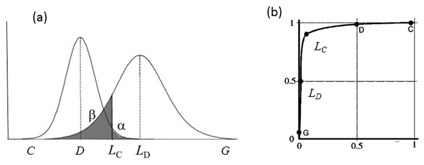
In order to evaluate the discrimination capacity of the different equations, that is, the ability to differentiate between presence or absence of yellow stain rather than to determine the percentage present, we used detection probability (also termed true positive or sensitivity) and false positive probability (1-specificity) by means of the critical level (LC), the limit of detection (LD) and the receiver operating characteristics (ROC) curves. These concepts are related through the distribution of outcomes, more specifically, the mean and the standard deviation of those distributions ([13]). When performing a discriminate test in a certain population in which one part of this population has a disease (or anomaly) and the other part does not, we would not expect to observe a perfect separation between the two groups but rather, the distribution of the test results will overlap (Fig. 2a). As regards the population with the disease, two cases are possible: true positive or sensitivity, when cases are correctly classified as positive and false negative or error type II, when cases are wrongly classified as negative (values higher than LC). Similarly, two cases are also possible for the population without disease: true negative or specificity, when cases are correctly classified as negative and false positive or error type I when cases are wrongly classified as positive (values lower than LC).
Fig. 2 - (a) Example plots of the probability distributions of total samples with disease (right) and number of samples without disease (left). (LC): critical level; (LD): limit of detection; (α): probability of committing a type I or false positive error (analysis of a white gives a positive yellow stain); (β): probability of making a type II or false negative error (analysis of a sample with yellow stain gives a negative yellow stain). Modified from Boqué ([3]). (b) The corresponding receiver operating characteristic (ROC) curves for the distributions shown in (a). Modified from Knoll ([13]).
In our case, critical level (LC - eqn. 1) and limit of detection (LD - eqn. 2) were calculated as follows ([3]):
where t1-α, v is the value of a t-Student distribution for a level of significance α and v degrees of freedom, and s0 is the estimate of the standard deviation when yellow stain is not present in the sample. Critical level and limit of detection were calculated for the three best equations.
ROC curves represent sensivity vs. 1- specificity (Fig. 2b), according to a particular critical level or decision threshold. The area under this curve (AUC) measures the accuracy of the detection system. The closer the curve to the upper left corner of the graph, the greater the accuracy of the calibration ([34]). The AUC statistic is a threshold-independent measure of the accuracy of the discriminant equation, in which values equal to or less than 0.5 indicate no discrimination, values between 0.7-0.8 indicate an acceptable discriminating capacity, and values between 0.8-0.9 or higher indicate excellent discriminations ([10]). A total of 7 ROC curves were calculated for the best equation, varying the size of the subpopulation that is compared with the subpopulation of 15 white samples. In the first calculation, all samples are used, while in the last one only those with 5% of yellow stain are entered.
Results and discussion
Spectra
Fig. 3 shows the mean spectra obtained for each of the different percentages of yellow stain in the zone with the absorption peaks. As far as we know, the spectra obtained in this study are the first spectra of cork granulate with different percentages of yellow stain in the near infrared zone. The spectra show the characteristic bands reported in previous studies on cork plank, stoppers or granulate, corresponding to -CH, -OH and C=O groups. Specifically, bands of 8230 and 5714 cm-1 correspond to the second and the first overtone of -CH groups. Bands of 6890 and 5180 cm-1 belong to the first overtone and combination bands of the -OH group. The band of 4650 cm-1 corresponds to the combination bands of the -CH and C=0 groups. Lastly, 4350 and 4240 cm-1 bands are associated with the combination bands of the -CH groups ([18], [19], [20], [21], [25]).
Fig. 3 - Mean spectra for each percentage of yellow stain (0, 5, 10, 15, 25, 35, 50 and 100%) in the zone with the absorption peaks.
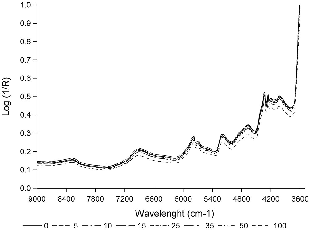
All spectra show the same absorption bands though the intensity differs for each of them. The spectrum of 100% yellow stain shows the highest absorption, spectra of 0, 5, 10, 15, 25 and 35% show the lowest absorption and the spectrum of 50% shows an intermediate absorption. Therefore, the absorption decreases as the percentage of yellow stain declines.
Calibration equations
Tab. 1 shows the statistics for the three best NIRS calibration equations. Equation 1 was developed using the entire NIRS region, without any preprocessing of the spectra. Equation 2 was developed using standard normal variate (SNV) spectrum preprocessing and also used the whole NIRS region. The last equation (Equation 3) was developed using only part of the NIRS region, 9400-4250 cm-1, using SNV preprocessing of the spectra. This region of the near infrared coincides with the absorption peaks previously described. No spectral outliers appeared in any of the three equations, nor were there samples classified as chemical anomalies.
Tab. 1 - Statistics obtained for the three best NIRS calibration equations. Number of PLS vectors (Rank), root mean square error of cross validation (RMSECV), coefficient of determination (R²), residual prediction deviation (RPD) and systematic error (BIAS).
| Equation | Rank | RMSECV (%) | R2 (%) | RPD | BIAS |
|---|---|---|---|---|---|
| Equation 1 | 8 | 3.28 | 98.86 | 9.35 | 0.0356 |
| Equation 2 | 6 | 3.16 | 98.93 | 9.68 | 0.0377 |
| Equation 3 | 8 | 2.34 | 99.42 | 13.10 | -0.0429 |
The number of PLS vectors or rank was 8 for Equations 1 and Equation 3 and was 6 for Equation 2. Fig. 4 shows the evolution of RMSECV as the ranking for Equation 3 increased. As can be seen, from rank 8 onwards, the RMSECV increases slightly.
Fig. 4 - Root mean standard error of cross validation (RMSECV) versus number of PLS vectors (Rank) for Equation 3.
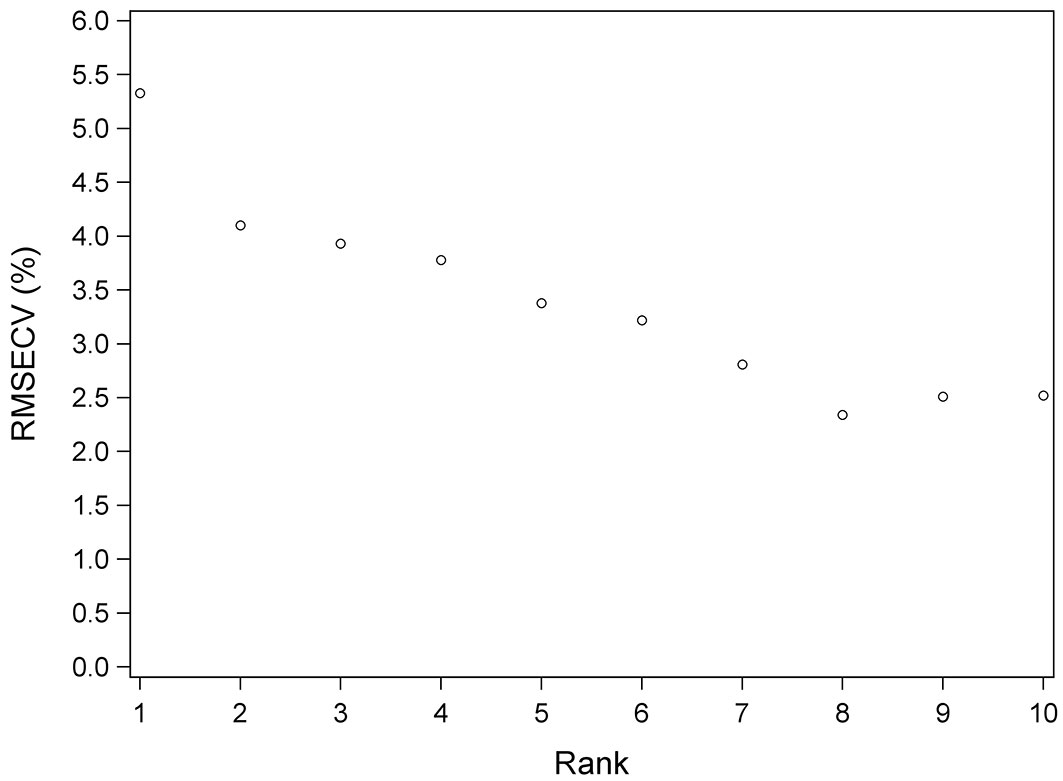
The RMSECV obtained in the three equations was similar and ranges from 3.28% (Equation 1) to 2.34% (Equation 3), revealing that the equations developed predict the percentage of yellow stain with a high level of precision. The R2 was greater than 98% for Equations 1 and Equation 2, and greater than 99% for Equation 3, so more than 98% and 99% respectively of the data variability is explained by the equations. The RPD values were above 8 (between 9.35-9.68) for Equations 1 and Equation 2, indicating that the equations are satisfactory for quality assurance (QA). In Equation 3, the RPD value was above 13 (13.1), indicating that the equation is like the reference ([33]). The BIAS values were positive for Equations 1 and Equation 2, and negative for Equation 3. A negative BIAS indicates that the equation overestimates the percentage of yellow stain, which is preferable as it provides greater assurance when estimating an anomaly.
Fig. 5 shows the percentages of yellow stain predicted by the equation vs. the real values for each of the samples in the case of Equation 3. It also shows the prediction limit and the confidence limit to 95% and the regression line (y = 0.21 + 0.99·x). It can be observed that the estimated values display a compact distribution around the real value, evidencing the accuracy of the calibration. All samples were within the 95% prediction limits except for three, one of 5%, another of 25% and another of 50% yellow stain. As regards the samples with 15% or less yellow stain (in industry, yellow stain is always found in low percentages, so this is the level of most interest), all samples were within the 95% prediction limits, except for the 5% yellow stain sample mentioned above.
Fig. 5 - Predicted values versus actual values for Equation 3. Solid line represents the regression line. Dark-shaded region shows the 95 % confidence interval and dashed lines are upper and lower 95 % prediction intervals of the regression.
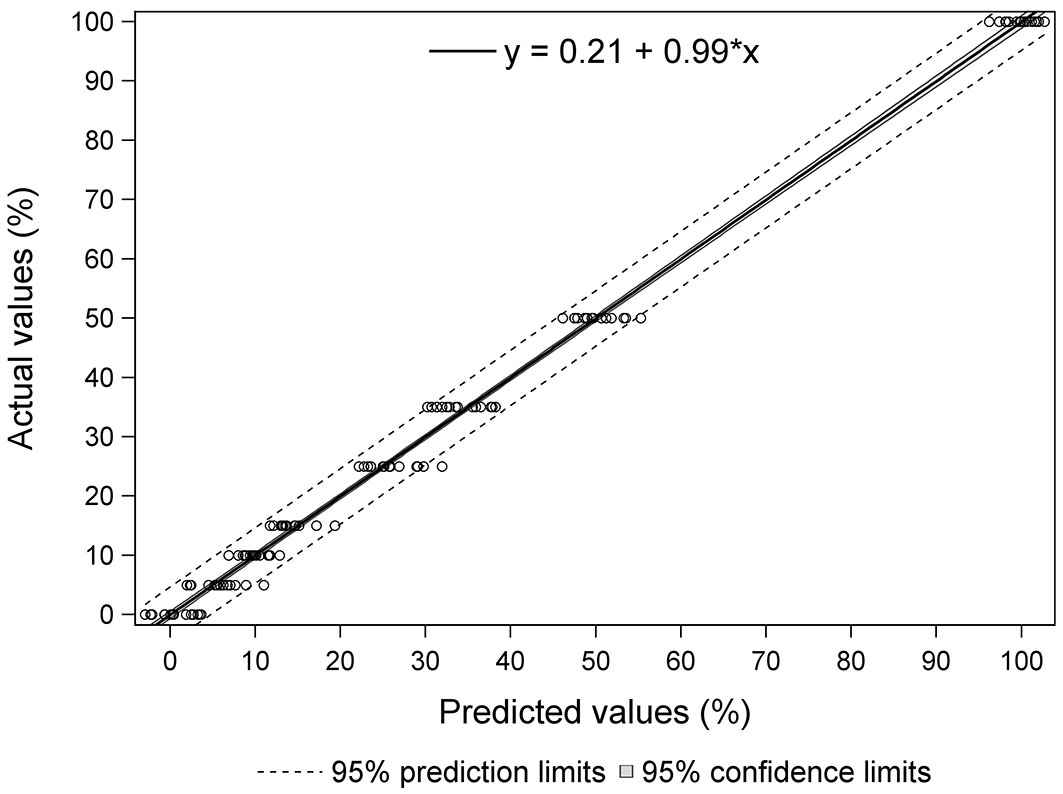
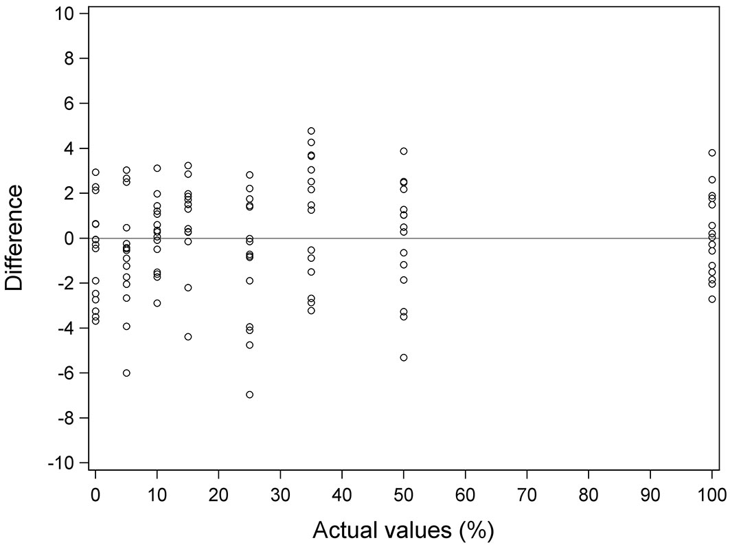
Fig. 6 shows actual values vs. the difference between actual and predicted values for each of the samples in the case of Equation 3. For most of the samples the difference between the actual and the predicted value was less than 3.5% in absolute value. Only three samples presented a difference greater than 5% in absolute value (-5.31% for the 50% yellow stain sample, -6.00% for the 5% sample and -6.96% for the 25% sample). These three samples correspond to those that are beyond the 95% prediction limits. It is important to note that the largest differences are associated with overestimates (preferable when estimating an anomaly). The biggest difference due to underestimation was 4.78 for a sample with 35% yellow stain. In the case of samples with 15% or less yellow stain, the biggest difference due to underestimation was 3.24% for a sample with 15% yellow stain.
Fig. 6 - Actual values vs. difference values for Equation 3. Difference values is the difference between actual values and predicted values. Solid line represents the reference line y=0.
Discrimination capacity of the calibration equations
To calculate the critical level and the limit of detection it is necessary to estimate the standard deviation of the predicted values for the 15 samples with 0% yellow stain for each of the equations (s0). These were 4.2%, 3.7% and 2.2% respectively. Tab. 2 shows the results for the critical level (LC) and the limit of detection (LD) for the three equations.
Tab. 2 - Critical level (LC) and limit of detection (LD) for the three best NIRS calibration equations. (s0): standard deviation of the predicted values for samples with 0% yellow stain for each of the equations.
| Equation |
s
0
|
LC (%) |
LD (%) |
|---|---|---|---|
| Equation 1 | 4.2 | 7.4 | 14.8 |
| Equation 2 | 3.7 | 6.5 | 13.0 |
| Equation 3 | 2.2 | 3.8 | 7.6 |
The best result for critical level and limit of detection was also obtained with Equation 3. The critical level was 3.8%. Therefore, if the predicted value of yellow stain is higher than 3.8%, then it will certainly not correspond to a white sample and yellow stain will be present at a 95% confidence level. There is a 5% probability of committing a type I or false positive error (analysis of a white sample giving a positive for yellow stain).
The limit of detection is 7.6%, meaning that this the minimum percentage of yellow stain for which we are able to state at a 95% confidence level that the sample is not white. As described in the previous section, there is a 5% probability of making a mistake, but in this case, it would be a false negative error (analysis of a sample with yellow stain gives a negative yellow stain).
Fig. 7 shows the different receiver operating characteristic (ROC) curves calculated for Equation 3 and its evolution when the number of samples with yellow stain is reduced. As can be seen, the equation has a very high discrimination capacity, since all curves are very close to the upper left corner. When decreasing the number of samples used to calculate the ROC curves (in Fig. 7 this is equivalent to moving from left to right and from top to bottom), and therefore using lower percentages of yellow stain for the calculation, the discrimination capacity remains high, only decreasing very slightly. The ROC curve calculated using only the 0 and 5% yellow stain samples is that which is of most interest because the amount of yellow stain present in the production lines is always small, since most of the defective part is removed prior to entering the factory. It can be observed that it maintains a very good discrimination capacity.
Fig. 7 - Receiver operating characteristic (ROC) curves for Equation 3. From left to right and from top to bottom: ROC curve with all samples; ROC curve with samples of 0-50%; ROC curve with samples of 0-35%; ROC curve with samples of 0-25%; ROC curve with samples of 0-15%; ROC curve with samples of 0-10%; and ROC curve with samples of 0-5%. The area under the curve (AUC) is showed for each of the calculated ROC curves.
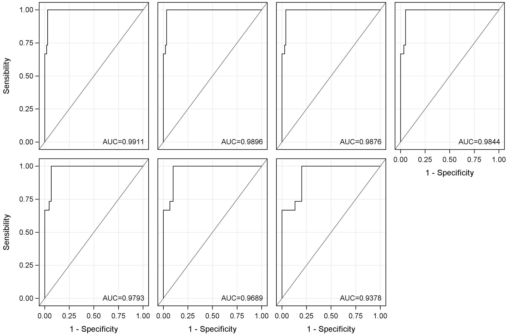
In addition to the graphical interpretation of the ROC curves, the area under the ROC curve (AUC) has also been calculated. The AUC values are between 0.9378 and 0.9911. This statistic confirms that the discrimination capacity of Equation 3 is very high, since values above 0.9 are considered excellent ([10], [30]).
The results obtained demonstrate that the NIRS technology is able to detect the presence of yellow stain and consequently an application able to detect continuously the presence of this anomaly in the lines of granulates industries could be developed. However, it must be taken into account that the models were obtained using just one geographical origin (Catalonia, Spain) and one granulometry (0.5-1 mm). Therefore, in order to generalize the model on a broader scale, different geographical origins and granulometries should be employed.
Conclusion
This study evidences the suitability of near infrared spectroscopy (NIRS) as a viable technique for detecting yellow stain in cork granulate. The NIRS equations obtained have a coefficient of determination (R2) between 98.86% and 99.42%, a root mean standard error of cross validation (RMSECV) ranging from 3.28% to 2.34% and a residual prediction deviation (RPD) above 9. The best result is achieved using standard normal variate (SNV) as preprocessing spectra, entering data exclusively from the near infrared region lying between 9400 cm-1 and 4250 cm-1. This region coincides with the principal absorption peaks of cork granulate. The critical level (LC) for the best equation is 3.8%, so percentages of yellow stain above 3.8% can be detected at a 95% confidence level. The limit of detection (LD) is 7.6%, meaning that this value is the minimum percentage of yellow stain that allows to state with 95% confidence that the sample is not white.
The receiver operating characteristic (ROC) curves show a high discrimination capacity. This capacity is maintained even when samples with a high content of yellow stain are progressively removed. The ROC curve calculated using only 0 and 5% yellow stain samples still shows a high discrimination capacity. Bearing in mind that most of the cork contaminated with yellow stain is removed in the post-harvest preprocessing, it is important that the equations maintains its discrimination capacity even at the lower percentages given that the presence of this anomaly is always low in cork used for the production of wine stoppers.
The results suggest that NIRS technology may provide a useful method for detecting low concentrations of yellow stain in cork granulate. Batches in which the anomaly has been detected could then be removed at the start of the production line, thus assuring the production of yellow-stain-free cork stoppers. However, further research must be undertaken focusing particularly on the lower percentages of yellow stain in order to improve the accuracy of this technique.
Acknowledgements
The authors would like to thank the INIA-CIFOR Cork Laboratory assistants María Luisa Cáceres and Lorenzo Ortiz Buiza for all their work in the laboratory.
References
Gscholar
Gscholar
Gscholar
Gscholar
Gscholar
Gscholar
Gscholar
Gscholar
Gscholar
Gscholar
Gscholar
Gscholar
Gscholar
Gscholar
Gscholar
Authors’ Info
Authors’ Affiliation
Mariola Sánchez-González
INIA-CIFOR, Ctra. de La Coruña km 7.5, E-28040 Madrid (Spain)
MONTES (School of Forest Engineering and Natural Environment), Universidad Politécnica de Madrid, C/ José Antonio Novais s/n, E-28040 Madrid (Spain)
Corresponding author
Paper Info
Citation
Pérez-Terrazas D, González-Adrados JR, Sánchez-González M (2018). Feasibility study of near infrared spectroscopy to detect yellow stain on cork granulate. iForest 11: 111-117. - doi: 10.3832/ifor2563-010
Academic Editor
Piermaria Corona
Paper history
Received: Jul 25, 2017
Accepted: Dec 12, 2017
First online: Jan 31, 2018
Publication Date: Feb 28, 2018
Publication Time: 1.67 months
Copyright Information
© SISEF - The Italian Society of Silviculture and Forest Ecology 2018
Open Access
This article is distributed under the terms of the Creative Commons Attribution-Non Commercial 4.0 International (https://creativecommons.org/licenses/by-nc/4.0/), which permits unrestricted use, distribution, and reproduction in any medium, provided you give appropriate credit to the original author(s) and the source, provide a link to the Creative Commons license, and indicate if changes were made.

Web Metrics
Breakdown by View Type
Article Usage
Total Article Views: 48014
(from publication date up to now)
Breakdown by View Type
HTML Page Views: 39797
Abstract Page Views: 3425
PDF Downloads: 3670
Citation/Reference Downloads: 15
XML Downloads: 1107
Web Metrics
Days since publication: 3068
Overall contacts: 48014
Avg. contacts per week: 109.55
Article Citations
Article citations are based on data periodically collected from the Clarivate Web of Science web site
(last update: Mar 2025)
Total number of cites (since 2018): 1
Average cites per year: 0.13
Publication Metrics
by Dimensions ©
Articles citing this article
List of the papers citing this article based on CrossRef Cited-by.
Related Contents
iForest Similar Articles
Research Articles
Characterization of technological properties of matá-matá wood (Eschweilera coriacea [DC.] S.A. Mori, E. odora Poepp. [Miers] and E. truncata A.C. Sm.) by Near Infrared Spectroscopy
vol. 14, pp. 400-407 (online: 01 September 2021)
Research Articles
Validation of models using near-infrared spectroscopy to estimate basic density and chemical composition of Eucalyptus wood
vol. 17, pp. 338-345 (online: 03 November 2024)
Research Articles
Selection of optimal conversion path for willow biomass assisted by near infrared spectroscopy
vol. 10, pp. 506-514 (online: 20 April 2017)
Research Articles
Estimation of total extractive content of wood from planted and native forests by near infrared spectroscopy
vol. 14, pp. 18-25 (online: 09 January 2021)
Research Articles
NIR-based models for estimating selected physical and chemical wood properties from fast-growing plantations
vol. 15, pp. 372-380 (online: 05 October 2022)
Research Articles
Comparison of extractive chemical signatures among branch, knot and bark wood fractions from forestry and agroforestry walnut trees (Juglans regia × J. nigra) by NIR spectroscopy and LC-MS analyses
vol. 15, pp. 56-62 (online: 08 February 2022)
Research Articles
Density, extractives and decay resistance variabilities within branch wood from four agroforestry hardwood species
vol. 14, pp. 212-220 (online: 02 May 2021)
Research Articles
Changes in moisture exclusion efficiency and crystallinity of thermally modified wood with aging
vol. 12, pp. 92-97 (online: 24 January 2019)
Research Articles
Visible and near infrared spectroscopy for predicting texture in forest soil: an application in southern Italy
vol. 8, pp. 339-347 (online: 09 September 2014)
Research Articles
Improving dimensional stability of Populus cathayana wood by suberin monomers with heat treatment
vol. 14, pp. 313-319 (online: 01 July 2021)
iForest Database Search
Search By Author
Search By Keyword
Google Scholar Search
Citing Articles
Search By Author
Search By Keywords
PubMed Search
Search By Author
Search By Keyword


