Visible and near infrared spectroscopy for predicting texture in forest soil: an application in southern Italy
iForest - Biogeosciences and Forestry, Volume 8, Issue 3, Pages 339-347 (2015)
doi: https://doi.org/10.3832/ifor1221-007
Published: Sep 09, 2014 - Copyright © 2015 SISEF
Research Articles
Abstract
Texture is a primary variable affecting the total amount of carbon stock in the soil. The standard methods for determining soil texture, however, are still conducted manually and are largely time-consuming. Reflectance spectroscopy in the visible, near infrared (Vis-NIR, 350-2500 nm) spectral region could be an alternative to standard laboratory methods. The aim of this paper was to develop calibration models based on laboratory Vis-NIR spectroscopy and PLSR analysis to estimate the texture (sand: 2-0.05 mm; silt: 0.05-0.002 mm; clay: <0.002 mm) in a forest area of southern Italy. An additional objective was to produce continuous maps of sand, silt and clay through a geostatistical approach. Soil samples were collected at 235 locations in the study area, and then dried, sieved at 2 mm and analyzed in laboratory for soil texture and Vis-NIR spectroscopic measurements. Spectra showed that soil samples could be spectrally separable on the basis of classes of texture. To establish the relationships between spectral reflectance and soil texture (sand, silt and clay) partial least squared regression (PLSR) analysis was applied to 175 soil samples, while the remaining 60 samples were used to validate the models. The optimum number of factors to be retained in the calibration models was determined by leave-one-out cross-validation. Results of cross validation of calibration models indicated that the models fitted quite well and the values of R2 ranged between a minimum value of 0.74% for silt and a maximum value of 0.84 for sand content. Results for validation were satisfactory for sand content (R2=0.81) and clay content (R2=0.80) and less satisfactory for silt content (R2=0.70). Geostatistics coupled with Vis-NIR reflectance spectroscopy allowed us to produce continuous maps of sand, silt and clay, which are of critical importance for understanding and managing forest soils.
Keywords
Forest Soils, Soil Texture, Vis-NIR Spectroscopy, Geostatistics, Southern Italy
Introduction
Carbon storage in forest ecosystems involves carbon in biomass and soil. Interest in the ability of forest soils to sequester atmospheric CO2 derived from fossil fuel combustion has recently increased because of the threat of climate change ([29]). Therefore, understanding the mechanisms and factors of organic carbon dynamics in forest soils is important for identifying and enhancing natural sinks for carbon sequestration, in order to mitigate the effects of climate change ([29]). The key factors in estimating the potential for organic matter in soil to act as a source or sink of CO2 are the size of the carbon flux into and out to the soil pool, and the residence time of organic matter in the soil ([43]). In relation to the second factor, it is critical to understand how texture and mineralogy influence the residence time of carbon in forest soils. Besides the key role in belowground carbon storage in forest ecosystems, soil texture strongly influences the availability and retention of nutrients, particularly in highly weathered soils ([48]).
Texture refers to the size and distribution of primary soil particles and it is the relative proportion of sand (2-0.05 mm), silt (0.05-0.002 mm), and clay (< 0.002 mm) in a given soil, inherited from the parent materials. Soil texture, which originates through weathering and pedogenetic processes ([38]), is not usually changed by land management practices, but it may be altered by erosion, deposition, truncation, landfill, etc. ([7], [38]).
Standard methods for determining texture in soils are either the pipette method or the hydrometer method, which are both conducted manually, being hence labor intensive and time-consuming.
Reflectance spectroscopy in the visible, near infrared (Vis-NIR, 350-2500 nm) spectral region could be an alternative to standard laboratory methods, even though soil Vis-NIR spectra are largely non-specific, quite weak and broad due to overlapping absorptions of soil constituents, often present at small concentrations in the soil ([56]). The method is based on the simplified assumption that the soil reflectance in the 350-2500 nm spectral region is a linear combination of the spectral signatures of its compositional components weighted by their abundance ([17], [3], [22]). Therefore, changes in chemical, physical and mineralogical properties of the soil produce distinct spectral features detectable through reflectance spectroscopy ([20], [31], [42], [36], [53], [2], [13], [14], [15]).
Vis-NIR spectroscopy requires only a few seconds to measure a soil sample, but the reflectance spectra are largely non-specific due to interference from the overlapping spectra of soil constituents that are themselves varied and interrelated ([55]). Consequently, the relevant information needs to be mathematically extracted from the spectra and correlated with soil properties. Generally, chemometric techniques and multivariate calibrations are used to this purpose ([32], [56], [45]), such as multiple linear regression (MLR), principal components regression (PCR), partial least-squares regression (PLSR) and artificial neural networks (ANN - [10], [42], [49], [63], [53], [21], [2], [34]).
Examples of the application of visible and near infrared spectroscopy for predicting soil clay content only, or the three textural fractions in soil (sand, silt and clay) can be found in Viscarra Rossel & McBratney ([52]), Sørensen & Dalsgaard ([47]), [35], Waiser et al. ([59]), Wetterlind et al. ([61]), Bricklemyer & Brown ([6]), Conforti et al. ([15]), Curcio et al. ([16]), [27], among others.
The representation of variability of textural fractions (sand, silt, and clay) is of critical importance for understanding and managing forest soils. Since such fractions are determined only at sampled locations, there is the need to couple the multivariate calibrations approach with geostatistical analysis to produce accurate continuous maps. Geostatistical methods ([33]) provide a valuable tool to study the spatial pattern of textural fractions, taking into account spatial autocorrelation of data to create mathematical models of spatial correlation structures, commonly expressed by variograms. The interpolation technique of textural fractions at unsampled locations, known as kriging, provides the “best”, unbiased, linear estimate of a regionalized variable in an unsampled location, where “best” is defined in a least-square sense ([11]).
The main objective of this paper was to develop, separately for each soil textural fraction, calibration models based on laboratory Vis-NIR spectroscopy and PLSR analysis in a forest area of southern Italy. An additio- nal objective was to use a geostatistical approach to map the three soil textural fractions (sand, silt and clay).
Material and methods
Study area
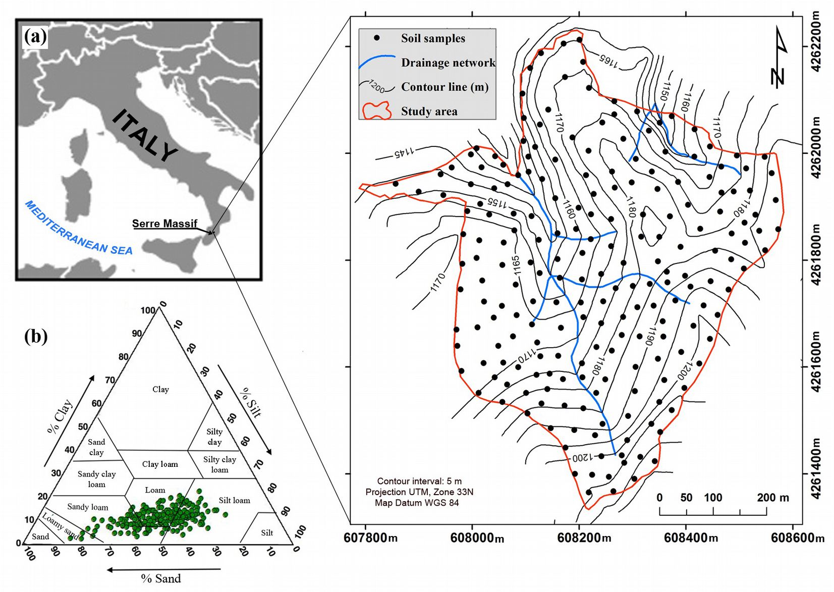
The study area is a high beech (Fagus sylvatica L.) forest of 332 000 m2, located in the Serre Massif (southern Italy - Fig. 1) from 16° 14′ 10″ E to 16° 14′ 42″ E of longitude and 38° 30′ 7″ N to 38° 29′ 31″ N of latitude. Elevation ranges from 1155 to 1205 m a.s.l. Slope ranges between 0 to about 45°, whereas the average slope is 10°.
Fig. 1 - (a) Study area and soil sampling locations; (b) soil textural triangle of the percentages of sand (2-0.05 mm), silt (0.05-0.002 mm) and clay (< 0.002 mm).
The climate is typical Mediterranean upland (Csb, sensu [28]) with a long-term (1928-2012) average annual precipitation of 1810 mm over 110 rainy days, and an average mean annual temperature of 11.3 °C. Yearly rainfall distribution exhibits a peak from November to February when more than 60% of total annual precipitation occurs.
Concerning the pedoclimate, the study area has a mesic soil temperature regime associated with an udic soil moisture regime ([1]).
The geology of the area is characterized by Palaeozoic granitoid rocks deeply fractured and weathered, frequently covered by thick regolith and/or colluvial deposits ([5], [9]). Morphologically, the study area is dominated by a mountains landscape with deep, V-shaped valleys and top paleosurfaces, representing the residual flat or gently-sloping highlands, often separated by steep slopes ([44], [8]).
Soils are relatively young, from poorly to moderately differentiated, and heavily dependent on the nature of the parent rock and the climatic conditions. Based on the USDA ([50]) soil classification, most of the soil types belong to Entisol and Inceptisol orders ([1]). The soil depth ranges from shallow to moderately deep (0.20 to 1 m) with profiles characterized by A-Bw-Cr horizons and/or A-Cr horizons ([1]). Moreover, the upper A horizon (Umbric epipedon - [50]) shows a very dark brown color due to the accumulation of organic matter.
Soil sampling
Soil samples were collected in October 2012 at 235 locations within the study area (Fig. 1a). Soil depth sampling was set at 0.20 m, measured from the base of organic horizons, which were removed. Soil was sampled in a metallic core cylinder with a diameter of 7.5 cm and height of 20 cm (883.6 cm3). Sampling locations were geo-referenced by a differential global positioning system (DGPS) with a precision of about 1 m.
Texture analysis
Prior to the texture analysis and Vis-NIR spectroscopic measurements, samples were oven dried at 45 °C for 48 hours in the laboratory, then gently crushed in an agate mortar to break up larger aggregates, afterward the visible roots were removed and each sample was sieved at 2 mm, homogenized and quartered. Such procedures allowed to homogenize the moisture and roughness of the soil samples, reducing their effect on the spectroscopic measurements.
The relative proportion of sand (2-0.05 mm), silt (0.05-0.002 mm), and clay (<0.002 mm) content was determined through the hydrometer method, after a pre-treatment with sodium hexametaphosphate as a dispersant ([40]). Then the texture was classified in accordance with the soil texture triangle of the United States Department of Agriculture ([50] - Fig. 1b).
Laboratory Vis-NIR spectroscopy
The soil samples sieved at 2 mm were placed in 9 cm diameter petri dishes and measures were taken in a black room (to better control irradiance conditions) with an ASD FieldSpec IV 350-2500 nm spectroradiometer (Analytical Spectral Devices Inc., Boulder, Colorado, USA). The instrument combines three spectrometers to cover the solar reflected portion of the spectrum between 350 and 2500 nm, with a sampling interval of 1.4 nm for the 350-1000 nm region and 2 nm for the 1000-2500 nm region. FieldSpec IV spectra were collected with a resolution of 1 nm, thus producing 2151 spectral bands. A 50-Watts halogen lamp with a zenith angle of 30°, located at a distance of approximately 25 cm from the soil sample was used as artificial illumination. The spectroradiometer was located in a nadir position at a distance of 10 cm from the sample, allowing radiance measurements to be carried out within a circular area of approximately 4.5-cm diameter. To minimize the noise level in the spectral signal, each soil reflectance spectra was recorded as the average of 50 scans carried out consecutively. In addition, to eliminate any possible spectral anomalies due to geometry of measurement, and minimize the possible errors associated with stray light, the measure was repeated 4 times, by rotating each sample 90 degrees (0, 90, 180 and 270 degrees) and the results averaged in post-processing.
A Spectralon panel (20 × 20 cm2, Labsphere Inc., North Sutton, USA) was used as white reference to compute reflectance values. Under the same measurement conditions a reference spectrum was acquired immediately before the first scan and after every set of five samples.
The average reflectance curves were translated from binary to ASCII with the VIEWSPECPRO® software (Analytical Spectral Devices, Inc., Boulder, CO, 80301) and re-sampled each 10 nm by reducing the number of wavelengths from 2151 to 216. Resampling smooths the spectra and reduces the risk of over-fitting ([26], [42]).
Multivariate statistical analysis
Before performing quantitative statistical analysis, spectral data pre-processing was performed to reduce noise and enhance the absorption frequencies ([32], [37]). The measured reflectance (R) spectra were transformed in absorbance through log(1/R) to reduce noise, offset effects, and to enhance the linearity between the measured absorbance and soil properties. The absorbance spectra were mean-centered to ensure that all results would be interpretable in terms of variation around the mean. Spectra were then smoothed using a Savitzky-Golay filter algorithm, with a second order polynomial and a window size of three, and transformed as first derivative to remove an additive baseline ([54]).
Partial least squares regression (PLSR - [23]), a common chemometric method in Vis-NIR analysis ([32], [53]), was chosen from the available multivariate statistical methods. The idea behind PLSR is to find a few linear combinations (components or factors) of the original X-values (spectral data) and to use only these combinations in the regression equation ([37]). In this way, the irrelevant and unstable information is discarded and only the most relevant part of the X-variation is used for regression; thus the problem of collinearity is solved and more stable regression equations are obtained ([37]). PLSR reduces the Vis-NIR matrix to a small number of statistically significant components. PLSR is based on latent variable decomposition of two sets of variables: the set X of predictors (matrix n × N, where n is the number of observations and N is the number of wavelengths) and the set y of response variable (vector n × 1 of sand or silt or clay). The latent variables, which are orthogonal factors maximizing the covariance between independent (X) and dependent variables (y), explain most of the variation in both predictors and responses. The optimal number of latent variables was chosen by a one-at-a-time cross-validation as the number that minimizes the predicted residual sum of squares.
Pre-treatment of data and the PLSR procedure were performed using the PARLES v. 3.1 software package developed by Viscarra Rossel ([54]).
To test the accuracy of the PLSR regression models the dataset was randomly split into two subsets: the calibration set (including 175 samples, i.e., 75% of the total dataset) for developing the prediction model, and the validation set (including 60 samples, i.e., 25% of the total dataset) to test the models’ accuracy.
To split the data randomly into two subsets, a value between 0 and 1 was generated simulating a uniform distribution in each sampling location. Then, by selecting the generated values greater than 0.75 a calibration set was created which included 75% of samples chosen randomly from the data. The complementary selection (values less than 0.25) was included in the validation set (25% of samples).
Leave-one-out cross-validation was used ([19]) to test the predictive significance of each PLSR component and to determine the number of factors (latent variables) to be retained in the calibration model. With the leave-one-out cross-validation one sample is left out of the global dataset and the model is calculated on the remaining data points. The value for the left-out sample is then predicted and the prediction residual computed. The above procedure is repeated until every sample has been left out once. To check the goodness of prediction of the leave-one-out cross-validation models, the coefficient of determination (R2) and the root mean square error (RMSE) were used. The best result for cross validation was considered that showing the lowest RMSE and the highest R2.
The models were independently tested through the validation set, and the coefficient of determination (R2val) and the root mean square error (RMSEval) were computed to check the goodness of prediction.
Geostatistical approach
To produce accurate continuous maps of each soil textural fraction, both measured and spectrally predicted values of sand, silt and clay were modeled as an intrinsic stationary process using a geostatistical approach ([11]). The quantitative measure of their spatial correlation was the experimental variogram γ(h), which is a function of the distance vector (h) of data pairs values separated by a lag vector h. A theoretical function, called variogram model, was fitted to the experimental variogram with the aim of building a model that captures the major spatial features of the attribute under study. The variogram model requires two main parameters: range and sill. The range is the distance over which pairs of the three soil texture fractions are spatially correlated, while the sill is the variogram value corresponding to the range. Optimal fitting was chosen on the basis of cross-validation, which checks the compatibility between the data and the model considering each data point in turn, removing it temporarily from the data set and using neighboring information to predict the value of the variable at its location. Goodness-of-fit for the model was based on the mean error (ME) and the mean squared deviation ratio (MSDR - [60]). ME values close to zero indicate unbiased estimates, whereas MSDR values close to 1 indicate a high model accuracy.
The fitted variograms for both measured and spectrally predicted values of sand, silt and clay were used to predict their values at the nodes of a 1 × 1 m interpolation grid by ordinary kriging ([60]). For more details, see Goovaerts ([24]), Chilès & Delfiner ([11]), Webster & Oliver ([60]), Wackernagel ([58]).
All statistical and geostatistical analyses were performed using the software package ISATIS®, release 2013.3 (⇒ http://www.geovariances.com).
Results and iscussion
The basic statistics for sand, silt and clay of exhaustive, calibration and validation sets are reported in Tab. 1. The sand content for the exhaustive data set ranges from 17.2 to 81.1 %, with a mean value of 42.6 %. Most soil samples have a moderate to high sand content and are generally poor in clay (Tab. 1). The silt content varies from 15.6 to 69.8 %, with a mean value of 45.6 %, while clay content ranges from 2.8 to 23 %, with a mean value of 11.5 %. Frequency distribution of the data appears quite symmetric, as revealed by the low values of skewness (Tab. 1).
Tab. 1 - Descriptive statistics of the exhaustive, calibration and validation data sets for the soil textural fractions.
| Textural fractions |
Data set | Count | Mean (%) |
Median (%) |
Minimum (%) |
Maximum (%) |
Standard deviation (%) |
Skewness |
|---|---|---|---|---|---|---|---|---|
| Sand (2-0.05 mm) |
Exhaustive | 235 | 42.6 | 42.3 | 17.2 | 81.1 | 11.4 | 0.55 |
| Calibration | 175 | 42.5 | 42 | 17.2 | 81.1 | 11.9 | 0.55 | |
| Validation | 60 | 43 | 43.1 | 23.2 | 72.4 | 9.8 | 0.55 | |
| Silt (0.05-0.002 mm) |
Exhaustive | 235 | 45.9 | 46 | 15.9 | 69.8 | 9.7 | -0.41 |
| Calibration | 175 | 46.1 | 47 | 15.9 | 69.8 | 9.9 | -0.51 | |
| Validation | 60 | 45.3 | 44.1 | 20.6 | 66 | 8.9 | -0.06 | |
| Clay (< 0.002mm) |
Exhaustive | 235 | 11.5 | 11.2 | 2.8 | 23 | 3.6 | 0.23 |
| Calibration | 175 | 11.5 | 11.2 | 2.8 | 23 | 3.6 | 0.21 | |
| Validation | 60 | 11.7 | 11.2 | 3.7 | 20.2 | 3.5 | 0.32 |
From the soil texture triangle (Fig. 1b), it appears that soil samples can be mainly classified as sandy loam, loam and silt loam. In addition, Tab. 1 shows that basic statistics for sand, silt and clay in the exhaustive, calibration and validation sets are very similar.
Spectral data analysis and PLSR prediction models for classes of soil texture
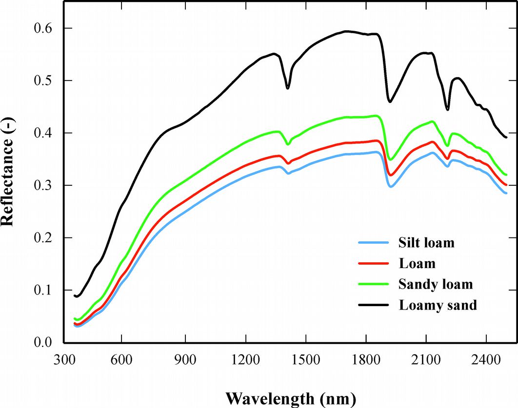
The Vis-NIR reflectance spectra of all soil samples shows the typical pattern for different wavelength bands responding to different chemical and/or mineralogical compositions or molecular groups ([18]). In particular, reflectance is generally lower in the visible range (400-700 nm) and higher in the near infrared (700-2500 nm) region, with three major specific bands around at 1400, 1900 and 2200 nm. These features can be associated with clay minerals, OH features of free water at 1400 and 1900 nm, and lattice OH features at 1400 and 2200 nm ([3], [53]). In addition, the spectra showed a small reflectance peak around 2200 nm, which may be due to organic molecules (e.g., CH2, CH3, and NH3), SiOH bonds, cation OH bonds in phyllosilicate minerals (e.g., kaolinite, montmorillonite - [12]).
Results of the visual inspection of spectral curves showed that variations in reflectance intensity and shape of the spectral curves can be due to differences in soil texture due to the correlation between the shape of NIR spectra and soil texture ([35]). Fig. 2 shows the mean spectral curves for different soil texture classes. Reflectance was relatively high for soils with loamy sand texture with over 70% sand content (Fig. 1). This was probably due to the high amount of quartz in the sand fraction, which raised the intensity of spectral reflectance ([62]). Conversely, the soil reflectance decreased when clay content dominated from phyllosilicates increased ([25], [39]) and, consequently, the organic carbon content increased ([41], [14]). Therefore, organic carbon is an important property as regards spectral behavior ([46], [4], [41], [14]). Generally, the reflectance of soil was found to be relatively low on account of the high content of organic carbon, throughout the Vis-NIR spectral domain.
Fig. 2 - Mean reflectance spectra for different soil texture classes.
Cross-validation results of the PLSR models for the three classes of texture are displayed in Fig. 3a. The prediction factors used in the calibration models, selected on the basis of the best cross validation results (lowest RMSE and the highest R2), were 12 for sand, 10 for silt and 9 for clay. Values of R2 ranged between a minimum value of 0.74 for silt and a maximum value of 0.84 for sand, indicating that the models fit quite well.
Fig. 3 - Scatter-plots of predicted vs. measured soil textural fractions for the calibration (a) and validation (b) data sets. (R2): coefficient of determination; (RMSE): root mean square error.
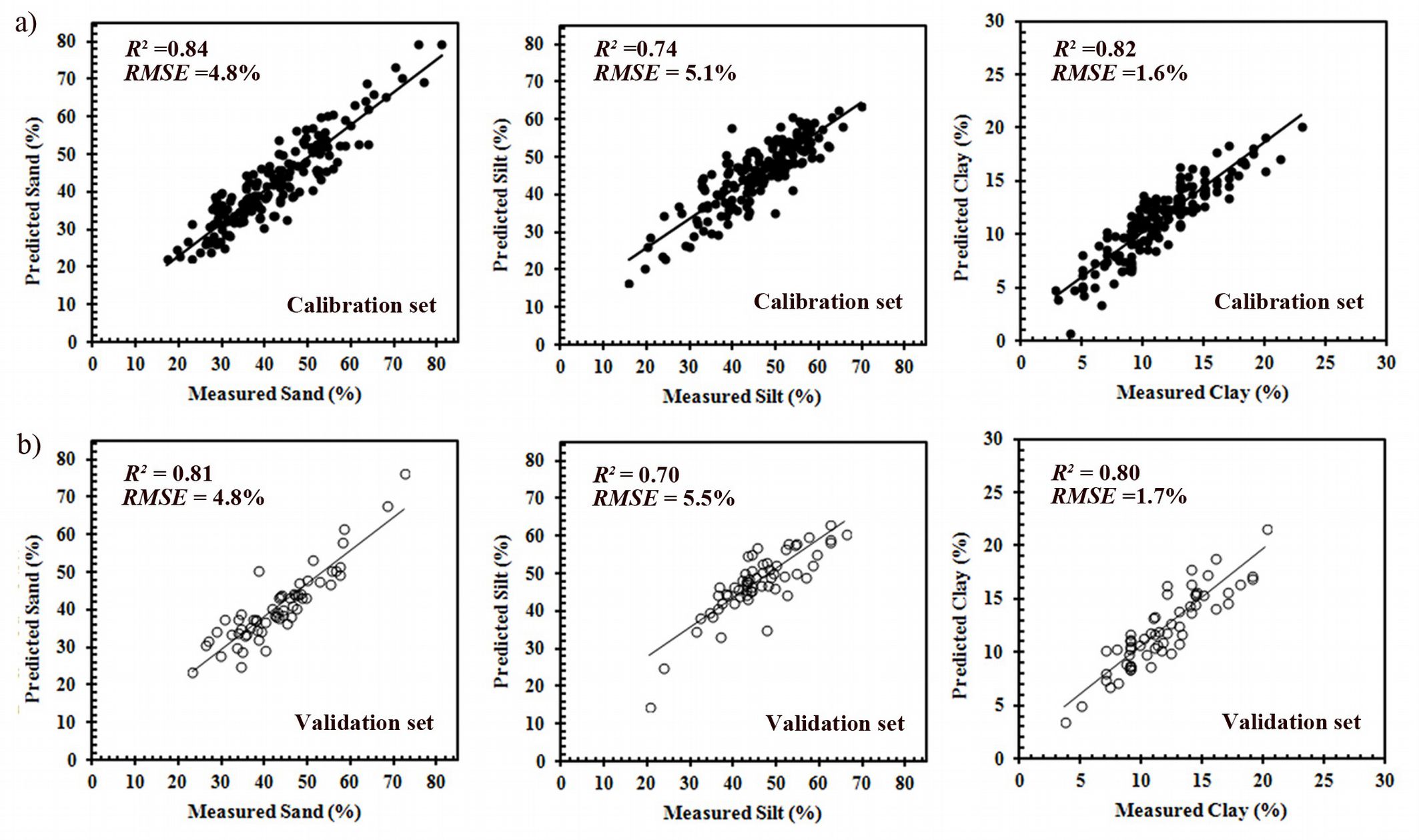
The validation of the models (Fig. 3b) gave satisfactory results for sand content (R2 = 0.81) and clay content (R2 = 0.80), but less stisfactory for silt (R2 = 0.70). Moreover, our results were in agreement with those obtained from the cross-validation prediction model, and from many other studies as well ([53], [57], [51], [16]).
Modeling of spatial dependence and mapping of classes of soil texture
Tab. 2 - Variogram model parameters for the values of measured (meas) and spectrally predicted (pred) textural fractions.
| Variable | Model | Range (m) | Sill (%) |
|---|---|---|---|
| Sandmeas | Nugget | - | 38 |
| Spherical | 44.06 | 64.91 | |
| Spherical | 290.06 | 26.05 | |
| Siltmeas | Nugget | - | 40.39 |
| Spherical | 46.85 | 42.17 | |
| Spherical | 279.6 | 11.64 | |
| Claymeas | Nugget | - | 4.39 |
| Spherical | 40.79 | 6.34 | |
| Spherical | 296.32 | 2.12 | |
| Sandpred | Nugget | - | 31.24 |
| Spherical | 52.98 | 54.75 | |
| Spherical | 291.37 | 32.99 | |
| Siltpred | Nugget | - | 21.42 |
| Spherical | 54.8 | 40.02 | |
| Spherical | 305.45 | 17.19 | |
| Claypred | Nugget | - | 3.99 |
| Spherical | 38.78 | 4.6 | |
| Spherical | 243.76 | 3.32 |
In the analysis of both measured and spectrally predicted sand, silt and clay contents, no anisotropy was evident in the 2-D variogram maps (not shown) up to a maximum lag distance of 450 m. Subsequently, a bounded isotropic nested variogram model was fitted for each experimental variogram. In the nested model, three basic structures (Tab. 2) were combined to include a nugget effect, a spherical model ([60]) at short range and a spherical model at longer range. The nugget effect is a positive intercept of the variogram and arises from errors of measurement and spatial variation within the shortest sampling interval ([60]). The spherical model ([60]) is given by (eqn. 1):
where c is the sill and a the range.
The presence of two ranges (short and long) in the nested model of the variogram means that the physical processes responsible for the variation of soil texture operate and interact at two spatial scales: the short range at about 40-50 m and the longer range at 280-300 m.
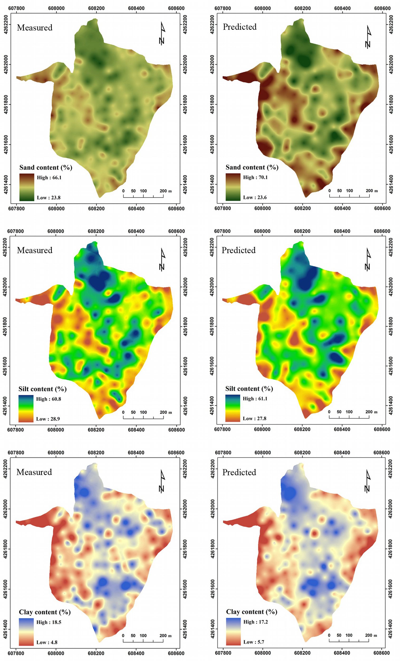
Cross-validation of the variogram models reported in Tab. 2 revealed satisfactory results, in terms of ME and MSDR (close to 0 and 1, respectively - data not shown). The fitted variogram models were then used with ordinary kriging to produce the maps of sand, silt and clay contents for the measured and spectrally predicted data (Fig. 4). Such maps showed a reasonable spatial similarity, with high and low values matching well (Fig. 4). High sand and low clay content were observed in the upper part of the slopes characterized by low gradient slope and poorly developed soils. Conversely, low values of sand and high content of fine particles (silt and clay) were prevalently observed along the foot of slopes and/or in concave areas where soils are deeper and more developed and, consequently, contain high levels of organic carbon.
Fig. 4 - Maps of measured (left) and spectrally predicted (right) values for sand (top panels), silt (middle panel) and clay (bottom panels) content in the soil of the study area. Map geographic coordinates are referred to the UTM zone 33N.
Comparing the interpolated maps of measured and spectrally predicted soil texture fractions, it is apparent that the PLSR predictions provided a good representation of the spatial pattern for sand, silt and clay content (Fig. 5). Moreover, as a spatial measure of prediction accuracy, maps of local mismatch were computed as the difference between the maps of measured and spectrally predicted values (Fig. 5). For sand content, 35.2% of the pixels were overestimated and 64.8% were underestimated, with a mean difference between measured and spectrally predicted sand content of 0.64% (min. -8.5%, max. 8.6%). For silt content, 71.6% of the pixels were overestimated and 28.4% were underestimated, with a mean difference between measured and spectrally predicted silt content of about -0.95% (min. -11.7%, max. 10.1%). As regards the clay content, overestimated pixels were 71.8% and 28.2% were underestimated; the mean difference between measured and spectrally predicted clay content was about -0.30% (min. -2.4%, max. 2.6%).
Fig. 5 - Maps of differences between measured and spectrally predicted values for sand (a), silt (b) and clay (c) content in the soil of the study area. Map geographic coordinates are referred to the UTM zone 33N.
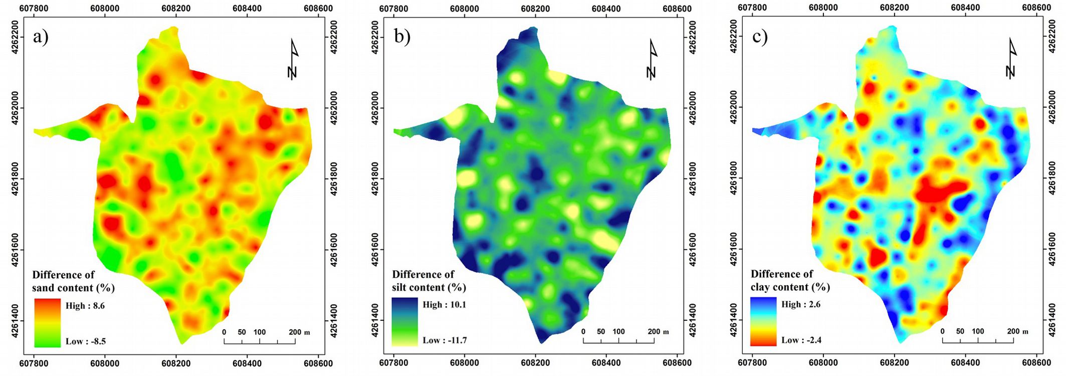
Based on the above results, it is clear that the maps of texture fractions could be used to aid land management decisions; in particular, maps of sand content could be used to identify areas with high drainage and those prone to accelerated nutrient leaching ([30]).
Conclusions
This study confirmed that soil Vis-NIR (350-2500 nm) reflectance spectra contain valuable information for predicting soil textural fractions (sand, silt, and clay content). Chemometrics techniques and multivariate calibration (PLSR) allowed researchers to extract the relevant information from the reflectance spectra and to correlate this with the soil texture fractions.
Results from cross validation of the calibration models revealed a quite good fitting, with R2 varying from a minimum value of 0.74% for silt to a maximum value of 0.84 for sand content. Also for validation, the results were satisfactory for sand content (R2 = 0.81) and clay content (R2 = 0.80) and less satisfactory for silt content (R2 = 0.70). Our results were in agreement with those obtained from the cross-validation prediction model, and from many other studies as well.
In conclusion, reflectance spectroscopy in the visible, near infrared (350-2500 nm) spectral region proved to be a useful alternative to laboratory standard methods for determining the soil textural fractions. By coupling the reflectance spectroscopy approach with geostatistical analysis, map of the spatial pattern for soil texture fractions were obtained, which can be used for better understanding and managing forest soils.
Acknowledgements
This work was supported by the project LIFE 09ENV/IT/000078 ManFor C.BD. “Managing forests for multiple purposes: carbon, biodiversity and socio-economic wellbeing” and by PONa3_00363 INFRASTRUTTURA AMICA: “Infrastruttura di Alta Tecnologia per il Monitoraggio Integrato Climatico-Ambientale”.
The authors thank two anonymous reviewers for their constructive comments on an earlier version of the manuscript. We are grateful to Nicola Ricca for assistance in the fieldwork, and Kevin O’Connel for the English revision of the manuscript.
References
Gscholar
Gscholar
Gscholar
Online | Gscholar
Gscholar
Gscholar
Gscholar
CrossRef | Gscholar
Online | Gscholar
Gscholar
Gscholar
Gscholar
Gscholar
Gscholar
Gscholar
Gscholar
Authors’ Info
Authors’ Affiliation
Raffaele Froio
Giorgio Matteucci
Gabriele Buttafuoco
Institute for Agricultural and Forest Systems in the Mediterranean (ISAFOM), National Research Council of Italy, v. Cavour 4/6, I-87036 Rende (CS, Italy)
Corresponding author
Paper Info
Citation
Conforti M, Froio R, Matteucci G, Buttafuoco G (2015). Visible and near infrared spectroscopy for predicting texture in forest soil: an application in southern Italy. iForest 8: 339-347. - doi: 10.3832/ifor1221-007
Academic Editor
Davide Ascoli
Paper history
Received: Dec 29, 2013
Accepted: May 29, 2014
First online: Sep 09, 2014
Publication Date: Jun 01, 2015
Publication Time: 3.43 months
Copyright Information
© SISEF - The Italian Society of Silviculture and Forest Ecology 2015
Open Access
This article is distributed under the terms of the Creative Commons Attribution-Non Commercial 4.0 International (https://creativecommons.org/licenses/by-nc/4.0/), which permits unrestricted use, distribution, and reproduction in any medium, provided you give appropriate credit to the original author(s) and the source, provide a link to the Creative Commons license, and indicate if changes were made.

Web Metrics
Breakdown by View Type
Article Usage
Total Article Views: 66320
(from publication date up to now)
Breakdown by View Type
HTML Page Views: 54989
Abstract Page Views: 4002
PDF Downloads: 5437
Citation/Reference Downloads: 92
XML Downloads: 1800
Web Metrics
Days since publication: 4311
Overall contacts: 66320
Avg. contacts per week: 107.69
Article Citations
Article citations are based on data periodically collected from the Clarivate Web of Science web site
(last update: Mar 2025)
Total number of cites (since 2015): 36
Average cites per year: 3.27
Publication Metrics
by Dimensions ©
Articles citing this article
List of the papers citing this article based on CrossRef Cited-by.
Related Contents
iForest Similar Articles
Research Articles
Availability and evaluation of European forest soil monitoring data in the study on the effects of air pollution on forests
vol. 4, pp. 205-211 (online: 03 November 2011)
Research Articles
Short-time effect of harvesting methods on soil respiration dynamics in a beech forest in southern Mediterranean Italy
vol. 10, pp. 645-651 (online: 20 June 2017)
Research Articles
Soil chemical and physical status in semideciduous Atlantic Forest fragments affected by atmospheric deposition in central-eastern São Paulo State, Brazil
vol. 8, pp. 798-808 (online: 22 April 2015)
Research Articles
Wood-soil interactions in soil bioengineering slope stabilization works
vol. 2, pp. 187-191 (online: 15 October 2009)
Research Articles
Soil stoichiometry modulates effects of shrub encroachment on soil carbon concentration and stock in a subalpine grassland
vol. 13, pp. 65-72 (online: 07 February 2020)
Research Articles
Seasonal dynamics of soil respiration and nitrification in three subtropical plantations in southern China
vol. 9, pp. 813-821 (online: 29 May 2016)
Research Articles
Changes in the properties of grassland soils as a result of afforestation
vol. 11, pp. 600-608 (online: 25 September 2018)
Research Articles
Soil fauna communities and microbial activities response to litter and soil properties under degraded and restored forests of Hyrcania
vol. 14, pp. 490-498 (online: 11 November 2021)
Research Articles
Relationship between microbiological, physical, and chemical attributes of different soil types under Pinus taeda plantations in southern Brazil
vol. 17, pp. 29-35 (online: 28 February 2024)
Research Articles
Effect of size and surrounding forest vegetation on chemical properties of soil in forest gaps
vol. 8, pp. 67-72 (online: 04 June 2014)
iForest Database Search
Search By Author
Search By Keyword
Google Scholar Search
Citing Articles
Search By Author
Search By Keywords
PubMed Search
Search By Author
Search By Keyword


