Geostatistical techniques for estimating aboveground biomass in eastern Amazonia
iForest - Biogeosciences and Forestry, Volume 19, Issue 2, Pages 85-93 (2026)
doi: https://doi.org/10.3832/ifor4789-018
Published: Mar 13, 2026 - Copyright © 2026 SISEF
Research Articles
Abstract
The Amazon plays a crucial role in global environmental debates due to its vital ecosystem services, including the carbon stock in its vegetation. Given the challenges of collecting field data in remote areas, remote sensing products such as those provided by the Global Ecosystem Dynamics Investigation (GEDI) mission are a valuable alternative for estimating aboveground biomass and carbon stocks, particularly in regions of high conservation interest. This study aimed to map aboveground biomass (AGB) and estimate carbon stocks in the Carajás Mosaic, a set of protected areas in eastern Amazonia, using geostatistical interpolation methods on GEDI-derived AGB data. We tested four methods: inverse distance weighting, ordinary kriging, regression kriging, and cokriging. Vegetation and terrain indices were evaluated as auxiliary variables. Results revealed high spatial variability in AGB, with significant correlations between AGB and spectral and terrain variables. Among the methods, regression kriging and cokriging showed a good spatial dependence structure, with cokriging providing the most accurate estimates. Overall, the results enabled a precise analysis of AGB estimates in these protected areas, providing insights into carbon distribution and emphasizing the importance of combining geostatistics and remote sensing for effective forest management and conservation planning.
Keywords
Spatial Variability, Remote Sensing, Protected Areas, Interpolation Methods
Introduction
The Amazon holds a central role in global environmental discussions due to the magnitude and importance of its ecosystem services ([3]), including climate regulation. Amazonian forests are estimated to store approximately 123 ± 23 Pg of Carbon in the above- and belowground biomass ([22]). However, recent estimates indicate that parts of the Amazon rainforest are undergoing critical ecological transitions, acting as a net carbon source ([14]). Ongoing deforestation and consequent carbon emissions contribute to global climate change and biodiversity loss, threatening endemic species ([24]) and negatively impacting the well-being of forest-dependent local communities ([16]).
Despite the importance of understanding carbon dynamics in tropical forests, the collection of accurate field data is hindered by high logistical costs and labor-intensive efforts ([30]). In this context, remote sensing data can be a viable alternative for monitoring aboveground biomass (AGB) ([26]), offering greater spatial and temporal coverage of this forested landscape. Among these technologies, Light Detection and Ranging (LiDAR) has proven particularly effective for obtaining accurate measurements of forest vertical structure across large areas ([11]). To enhance the accuracy of AGB estimates, integrated models that combine tree-level field and remote sensing data have been developed ([29]), enabling a more comprehensive assessment of forest contributions to climate change regulation.
Launched in 2019, the Global Ecosystem Dynamics Investigation (GEDI) was designed to retrieve vegetation structure information using a sampling design that explicitly quantifies AGB and its associated uncertainty ([10]). However, its discrete footprint-based data structure, comprising 25-m diameter footprints spaced about 60 m apart along-track and about 600 m between orbits ([10]), poses challenges for continuous spatial analysis ([8]). GEDI provides aggregated products with a spatial resolution of 1 km, which is insufficient for high-resolution AGB mapping and exacerbates the limitations imposed by the sparse sampling density.
Geostatistical techniques can be a viable approach to address the spatial discontinuity of GEDI data by enabling the interpolation of AGB values between sampled locations. These methods have been successfully applied to investigate spatial variation in vegetation structure, map forest variables, and support site-specific environmental assessments ([12]). By combining geostatistical models with remote sensing inputs and environmental covariates, several studies have enhanced the spatial prediction of forest attributes, employing methods such as ordinary kriging, regression kriging, or cokriging ([38], [20], [41], [46]). However, only Benítez et al. ([2]) have applied these techniques in the Amazonian context. Their results indicated that kriging was the most accurate method for spatializing AGB and emphasized the need to investigate which variables correlate more strongly with AGB across different Amazonian landscapes.
One of the most important forest remnants in the eastern Amazon is a group of neighboring, overlapping protected areas and indigenous lands that together encompass 1.21 million hectares, commonly referred to as the “Carajás Mosaic”. Despite their exceptional biodiversity, high levels of endemism, and natural capital ([7]), little is known about the spatial variation of their carbon stocks ([37]). However, recent studies have quantified the carbon stock potential in sample plots within the Carajás National Forest, which is part of the Carajás Mosaic, estimating up to 182.5 t C ha-1 in areas of open ombrophilous forest ([6]). These studies also identified the disproportionate role of large trees, which represent less than 1% of the inventoried individuals but account for 33% of the total carbon stock. Their findings highlight the need to integrate remote sensing data with field measurements efficiently to scale up carbon assessments across broader regions of the mosaic.
This study aims to generate a spatially explicit AGB map for natural forest areas within the Carajás Mosaic using GEDI data and geostatistical techniques. Four interpolation methods were tested and compared to identify the most suitable approach for addressing spatial gaps and improving AGB estimation. In addition to the geostatistical framework, we correlated AGB data with environmental variables to further enhance estimation accuracy. Using the best-performing method, we estimated the region’s total carbon stock and analyzed its spatial distribution to inform conservation planning.
Materials and methods
Study area
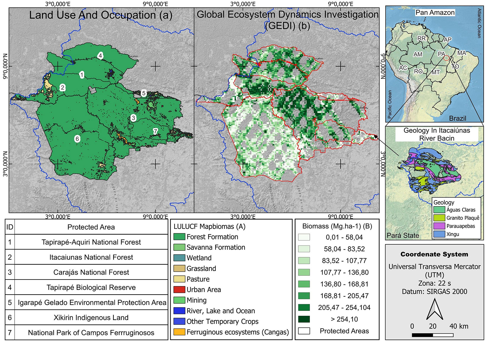
The study area consists of 1.21 million ha of the Carajás Mosaic, which includes two protected areas (PA) of integral protection, four of sustainable use, and the indigenous land of Xikrin do Cateté (Fig. 1). The limits were obtained from the environmental information database of the Brazilian Institute of Geography and Statistics (IBGE). The area is located in the Eastern part of Amazonia, in the state of Pará, and forms a fragment that is almost isolated from other preserved areas (PAs). In sustainable-use PAs, natural resources can be exploited as long as the use complies with environmental legislation, whereas in integral-protection PAs, resource extraction is prohibited, allowing only activities such as environmental education, research, and ecotourism.
The Xikrin, part of the Kayapó linguistic group, have been the original inhabitants of the region since ancient times. Comprising three villages, Cateté, the largest in both territory and population, Dju-djekô, and Ô-Odjã, the most recently founded with a smaller demographic, these settlements showcase a notably autonomous political organization. The official approval of the indigenous land of the Xikrins of Catété in 1991 marked a significant acknowledgment of their historical connection to the area.
The original vegetation of the Carajás Mosaic includes different physiognomies, predominantly ombrophilous forests, with 11.597.49 km2 (95.27%) of open and dense formations, and 82.57 km2 (0.006%) of rocky outcrop fields known as ferruginous “Canga”. The ferruginous “Canga” is directly associated with large iron ore deposits, revealing a strong influence of geology on vegetation and defining different geoenvironments ([37]). Nowadays, 3.78% of the area of the “Carajás Mosaic” has already been deforested and converted to mining areas and related infrastructure, mainly in the Carajás National Forest (based on the 2021 Mapbiomas project land-use classification). The climate is classified by Köppen as “Aw” with well-defined dry (May to October) and wet (November to April) seasons, including periods of torrential rains and monthly average temperatures between 19 and 31 °C ([1]).
Environmental variables in predictive AGB mapping
We used the AGB data provided by the GEDI L4B product, which consists of 1-km-resolution estimates of aboveground biomass density (AGB) based on observations from April 2019 to August 2021. It utilizes the GEDI L4A Footprint Biomass product to convert high-quality waveform data into AGB predictions and statistically infer the mean AGB within each 1 km cell ([13]). The GEDI instrument, launched in December 2018 aboard the International Space Station, conducts high-resolution laser samplings of Earth’s three-dimensional structure globally, covering latitudes between 51.6° N and 51.6° S, with the highest spatial resolution and density to date.
Vegetation and terrain indices were evaluated as predictors of AGB. The mean Normalized Difference Vegetation Index (NDVI), Normalized Difference RedEdge Index (NDRE), Soil-Adjusted Vegetation Index (SAVI), and Enhanced Vegetation Index (EVI) from 2019-2021 resolution were calculated using Landsat collection 8 data in the Google Earth® Engine (GEE). The terrain variables (altitude, slope, roughness, and aspect) were downloaded from the online Topodata Index Map of the National Institute for Space Research (INPE) with a resolution of 30 m. We calculated the minimum, maximum, standard deviation, median, mode, mean, and variance of predictor variables. Pearson’s correlation r was calculated to identify the most critical variables, and only those with significant correlations (r ≥ 0.50) were considered.
Since our focus is on calculating carbon stock in the natural forests of the Carajás Mosaic, only GEDI pixels with more than 70% of their area covered by primary forest were included in the predictor calculations. These areas were identified using the Mapbiomas land-use/land-cover classification data at 30 m spatial resolution from 1985 to 2021, and the methodology reported by Silva Junior et al. ([42]).
Although not used in the models, we assessed the influence of geology on the AGB within the Carajas Mosaic. The primary forest areas were categorized according to geological classes from the Information Database (Bdias) of the Brazilian Institute of Geography and Statistics (IBGE). Differences in mean AGB across the four geological typologies were evaluated using the Kruskal-Wallis and the Dunn test. These four typologies (Águas Claras, Granito Plaque, Parauapebas, and Xingu) accounted for over 80% of the AGB estimated by GEDI.
Geostatistics and spatial modeling techniques
Geostatistics provides techniques for estimating spatially structured variables. A key component is the semivariogram, which quantifies the correlation between samples as a function of distance. This allows nearby samples to exert more influence on predictions than distant ones, improving spatial accuracy ([19]).
The application of a theoretical mathematical model is essential for a comprehensive analysis, with key components such as nugget, sill, and range providing insights into spatial variance and modeling the ideal structure of the semivariogram for each variable. Here, we used four spatial modeling methods to fill data gaps in the GEDI mapping of AGB: one deterministic (Inverse Distance Weighted - IDW) and three stochastic approaches (Ordinary Kriging, Regression Kriging, and Cokriging). The GEDI dataset was split into training (70%) and validation (30%) subsets using the “caret” library in R ([33]). To ensure independence, a two-tailed Student’s t-test was performed between the subsets.
From this point onward, the techniques inverse distance weighting, ordinary kriging, regression kriging, and cokriging will be referred to by their abbreviations: IDW, OK, RK, and CK, respectively.
Inverse distance weighted (IDW)
IDW was performed with an exponent of 2, known as Inverse Square Distance. This approach is computationally efficient and may yield results similar to kriging when spatial structure is weak (IDE > 75% - [44]). However, where spatial structure is present, kriging is recommended because it does not introduce bias into the estimate.
Ordinary kriging (OK)
The OK method ([19]) assigns weights to observed values based on both spatial and statistical relationships, captured in the empirical semivariogram ([40]). The OK estimator is defined as (eqn. 1):
where Z(xi) is the value at location xi, h is the distance separating two samples, and N(h) is the number of sample pairs separated at each distance h. The resulting plot of γ(h) as a function of h allows for modelling spatial behavior.
Cokriging (CK)
CK is a multivariate geostatistical technique that predicts a primary variable based on its spatial correlation with one or more secondary variables. It is cost-effective and yields high-accuracy results when a strong correlation exists between variables ([47]).
Spatial dependence in CK is assessed using the cross-semivariogram, which evaluates the joint variability between the primary and secondary variables (eqn. 2):
where z(x) and Z2(x) represent the value of the primary and secondary variables at a specific location x.
Regression kriging (RK)
RK is a combination of two spatial interpolators: a global and stochastic model. The first concerns the application of a multiple linear regression model (MLR), which captures the behavior of the primary variable ([17]), in this case, AGB, as a function of spatial covariates. The residuals from this model, representing unexplained variation, are then interpolated using OK to enhance spatial prediction. The covariates tested (independent variables) included NDVI, NDRE, SAVI, EVI, Altitude, Slope, Roughness, and Aspect (see Appendix 1 in Supplementary material). Variables with non-significant correlation coefficients (p > 0.05) were excluded from the model. A Forward-Stepwise procedure was applied to identify the most influential predictors for the RK model.
The models were evaluated against fundamental statistical assumptions, including the normality of residuals (Breusch-Pagan test), independence of residuals (Durbin-Watson test), and multicollinearity (Variance Inflation Factor, VIF). Assessing normality is crucial, as distributions with pronounced skewness or heavy tails can compromise the validity of significance tests and reduce the robustness of parameter estimates.
Tab. 1 - Summary statistics of aboveground biomass (AGB ha-1) derived from the GEDI map with 1-km resolution for primary forest areas within the Carajás Mosaic. Outlier values were removed from the training dataset to avoid bias in the calculations. (yÌ„): mean value; (s): standard deviation; (s2): variance; (CV): coefficient of variation.
| Statistics | AGB (Mg ha-1) |
|---|---|
| Min | 3.45 |
| Max | 991.3 |
| Mode | 121 |
| ȳ | 148.2 |
| s | 81.58 |
| s2 | 6656.88 |
| CV (%) | 55.05 |
To mitigate potential spatial trends and ensure the validity of the intrinsic hypothesis of stationarity, the classical Matheron estimator with second-order correction was employed. The investigation of this assumption was conducted during the exploratory data analysis stage, and the full procedure is provided in Appendix 2 (Supplementary material). Three widely used semivariogram models (spherical, exponential, and Gaussian - Tab. 1) were fitted to the experimental semivariogram using weighted least squares. The same fitting procedure was applied to the residuals and predicted values of the multiple linear regression (MLR) model, following the residual kriging (RK-B) approach described by Odeh et al. ([28]). This approach integrates regression, which models the explained variation, with ordinary kriging, assuming a zero mean, to estimate the unexplained variation ([17]), as presented in eqn. 3:
where m(u) is the estimated mean (drift) through regression; r(u) is the estimated residual through kriging; β0 + β1 x(u) is the regression model; and λα is the kriging weights for residuals at neighboring points.
The RK-B approach was selected because the AGB data exhibited a well-defined spatial structure, as previously identified using OK.
Outliers were identified using Cook’s distance on standardized residuals, calculated with the “lm” package in R. Observations with Cook’s distance outside the range -3 to 3 were treated as leverage points and removed to improve model accuracy. These outliers were found to distort the overall trend of the data and weaken the observed correlation. Moreover, because both the predicted values and residuals were spatially analyzed, the presence of outliers could introduce artificial spatial dependence or conceal genuine spatial patterns.
Methods evaluation
A total of 3640 GEDI’s footprints (70%) were randomly selected to train the models for AGB prediction, while 862 pixels (30%) were reserved for model validation. Due to the spatially clustered acquisition of GEDI data, footprint distribution can be irregular, resulting in diamond-shaped gaps between adjacent orbits (see study location map). To minimize potential spatial sampling bias, 10 × 10 km rectangles were randomly distributed throughout the study area to simulate these GEDI gaps and generate an independent validation dataset.
The stochastic methods (OK, CK, RK) were evaluated using cross-validation procedures to identify the spatial model that best fits the empirical semivariogram. Evaluation metrics included the Akaike Information Criterion (AIC), Spatial Dependency Index (IDE), reduced mean error (RME), and the standard deviation of the reduced mean error (DRME) ([39]). Parameter estimation for the theoretical semivariogram models involved determining the nugget (τ2), sill (σ2), and range (φ). The SDI was calculated as the ratio τ2 / (τ2 σ2) with spatial dependence index (SDI) classified following Cambardella et al. ([4]) thresholds as strong (IDE < 25%), moderate (25% < IDE < 75%), and weak (IDE > 75%). All geostatistical analyses were performed using the GeoR package in R version 4.0.2 ([33]).
For quantitative comparison of AGB predictions generated by the deterministic IDW method and the stochastic approaches (OK, CK, RK), predicted values were compared to observed AGB measurements using Root Mean Squared Error (RMSE), Mean Absolute Error (MAE), and Mean Error (ME). A lower RMSE indicates reduced residual variance, whereas a lower MAE reveals an improved precision between predicted and observed AGB values. The ME assists in identifying any systematic bias in the model, and the RMSE expressed as a percentage contextualizes predictive accuracy relative to the observed data range. Consistently small values in these metrics suggest that the models are more aligned with the actual patterns of AGB distribution, providing a reliable estimate of AGB for spatial interpretation.
Additionally, to assess spatial consistency among models, the four interpolated AGB maps were compared using the Multivariate Band Collection Statistics tool, which performs a pixel-wise correlation analysis across the entire study area and produces a correlation matrix reflecting inter-map relationships. The selection of the optimal interpolation method for the Carajás Mosaic was based on an integrative assessment of both statistical performance and visual inspection of spatial patterns across training and validation datasets.
Results
Exploratory data analysis
The GEDI-estimated AGB for primary forests in the Carajás Mosaic revealed a high variability, ranging from 3.45 to 991.30 Mg ha-1, respectively (Tab. 1). The Shapiro-Wilk test for normality rejected the null hypothesis of a normal distribution (p-value = 2.2e-16).
Among the terrain variables, altitude (R2 = 0.46), slope (R2 = 0.50), and roughness (R2 = 0.50) showed the strongest correlations with AGB estimates. Due to multicollinearity between slope and roughness, slope was selected because it is easier to obtain and available in national databases. Aspect and curvature displayed the weakest correlations: -0.08 and -0.005, respectively.
As for spectral variables, EVI (R2 = -0.45), NDVI (R2 = -0.44), and SAVI (R2 = -0.54) demonstrated the strongest correlations, with SAVI selected for further analyses. NDRE showed the weakest correlation (R2 = 0.004), indicating limited potential for biomass prediction, despite being an adapted NDVI index.
Aboveground biomass modeling
Ordinary kriging
Exploratory spatial data analysis revealed no trends along latitude or longitude, confirming that geostatistical assumptions were satisfied, and the generated semivariograms are omnidirectional and isotropic.
For OK, the exponential model provided the best fit based on validation statistics (Tab. 2), with low RME and high DRME. The SDI indicated a robust spatial dependence structure due to the significant contribution and range values in relation to the nugget effect (Tab. 2). This index, which incorporates range to assess variability magnitude, showed that beyond a distance (h) of 6 km, AGB spatial behavior in the Carajás Mosaic presents a strong correlation at moderate distances.
Tab. 2 - Performance metrics of the models used to spatialize aboveground biomass (AGB) in the Carajás Mosaic: mean error (ME), mean absolute error (MAE), root mean square error (RMSE), and percentage of root mean square error (RMSE%) for both training and testing datasets. Reduced mean error (RME) derived from the comparison between the GEDI and the interpolated biomass maps generated by each method was presented. R2 is the Spearman’s linear correlation based on test data.
| Model | Statistics | AGB error (Mg ha-1) | RME | Spearman (R²) |
|
|---|---|---|---|---|---|
| Training dataset |
Test datasets |
||||
| IDW | ME | 0.10 | 18.45 | 0.51 | 0.64 |
| MAE | 0.01 | 0.06 | |||
| RMSE | 30.22 | 64.27 | |||
| RMSE (%) | 20.39 | 37.05 | |||
| Ordinary Kriging |
ME | 0.04 | 13.13 | 0.24 | 0.68 |
| MAE | 0.02 | 0.05 | |||
| RMSE | 42.92 | 58.80 | |||
| RMSE (%) | 28.96 | 33.89 | |||
| Regression Kriging |
ME | -0.24115 | 11.75323 | 0.21 | 0.65 |
| MAE | 0.050385 | 0.002088 | |||
| RMSE | 62.34477 | 60.19027 | |||
| RMSE (%) | 42.06542 | 34.69745 | |||
| Cokriging | ME | 0.051978 | 11.80091 | 0.21 | 0.70 |
| MAE | 0.028143 | 0.046773 | |||
| RMSE | 39.89416 | 56.8957 | |||
| RMSE (%) | 26.91 | 32.79825 | |||
Regression kriging (RK-B)
Among the environmental variables, the average slope and SAVI emerged as the most significant predictors of AGB values, with no evidence of multicollinearity, as assessed by the variance inflation factor (VIF = 1.075). Therefore, these variables were selected for inclusion in the RK-B model to predict AGB, resulting in the following equation (eqn. 4):
This RK-B model achieved an adjusted R2 (R2adj) of 0.42 and a standard error of 61.86 (Sxy). This model satisfied the assumptions of multiple regression, demonstrating normality of residuals according to the Shapiro-Wilk test (W = 0.98744, p-value = 0.0235) and homoscedasticity based on the Breusch-Pagan test (BP = 169.37, df = 2, p-value = 0.0137).
The regression residuals tend to be more dispersed for values exceeding 240 Mg ha-1, suggesting that prediction errors increase for very high AGB values. However, despite the correlation of 0.42 with GEDI data, the estimated values show a generally linear growth pattern, with lower errors in the average AGB range (66.77 to 233.25 Mg ha-1).
The experimental semivariograms derived from AGB estimation and regression residuals both exhibited a moderate spatial dependence index (SDI) according to the classification of Cambardella et al. ([4]). The exponential theoretical model provided the best fit for both data sets, although performance varied by data type. The estimated values contributed approximately half as much as the residuals, one-third of the nugget effect, and nearly twice the range (Tab. 3).
Tab. 3 - Main parameters of the isotropic experimental semivariogram for the ordinary (OK), regression kriging (RK), RK residuals (RKr), and cokriging (CK): nugget effect (τ), sill (σ2), and range (A), as well as model selection statistics; Akaike Information Criterion (AIC), Spatial Dependency Index (SDI), Reduced Mean Error (RME), and Deviation of Reduced Mean Error (DRME).
| Method | Model | τ | σ2 | A (m) | AIC | SDI | RME | DRME |
|---|---|---|---|---|---|---|---|---|
| OK | Exp | 1012.5 | 4062.2 | 6343.0 | -46503.9 | 35.27 | -0.00059 | 0.86421 |
| RKr | Exp | 998.0 | 2010.8 | 7045.6 | -47971.6 | 16.51 | -0.01660 | 0.85269 |
| RK | Exp | 389.1 | 1050.1 | 16854.1 | -46749.4 | 16.47 | -0.00177 | 0.92034 |
| CK | Exp | 40.0 | 220.0 | 40645.2 | -41058.5 | 37.94 | -0.00045 | 0.91245 |
Incorporating the spatial patterns of both residuals and predicted values enhanced the modeling framework, leading to more accurate AGB estimates by explicitly accounting for spatially correlated errors in the regression model. This approach highlighted regions with higher or lower AGB predictions. The model selection statistics showed satisfactory results, meeting the required criteria (Tab. 3). Notably, the DRME was higher than that for OK, suggesting that incorporating auxiliary variables into AGB prediction improved overall model performance.
Cokriging
The SDI revealed a strong spatial dependence for the CK model, and the selection statistics confirmed the accuracy of the modeling process, with DRME performing similarly to RK, emphasizing the importance of predictor variables in AGB estimation (Tab. 3). The cross-semivariogram exhibited the smallest nugget effect and contribution when compared to OK and RK. This result indicates that the interaction between variables reduced spatial variability arising from differences in their scales and spatial characteristics. AGB exhibits greater spatial variability, whereas the slope shows shorter, more defined variations across the study area, leading to a decrease in variability in the cross-semivariogram. In this case, the result underscores the importance of using slope as an auxiliary variable, as the resulting variability was lower than that of AGB but higher than that of the slope, indicating a partial gain between the two.
Comparison between biomass maps
The training and test datasets showed significant differences in AGB values (t-Student test, t=8, df=4500, p-value=2.345e-16), with averages of 173.47 and 148.20 Mg ha-1, respectively. For the training data, RK exhibited the highest negative systematic bias, indicating consistent underestimation of AGB values, as well as the highest RMSE (Tab. 2). In contrast, the IDW showed the lowest MAE and RMSE, suggesting that AGB predictions were closer to observed values.
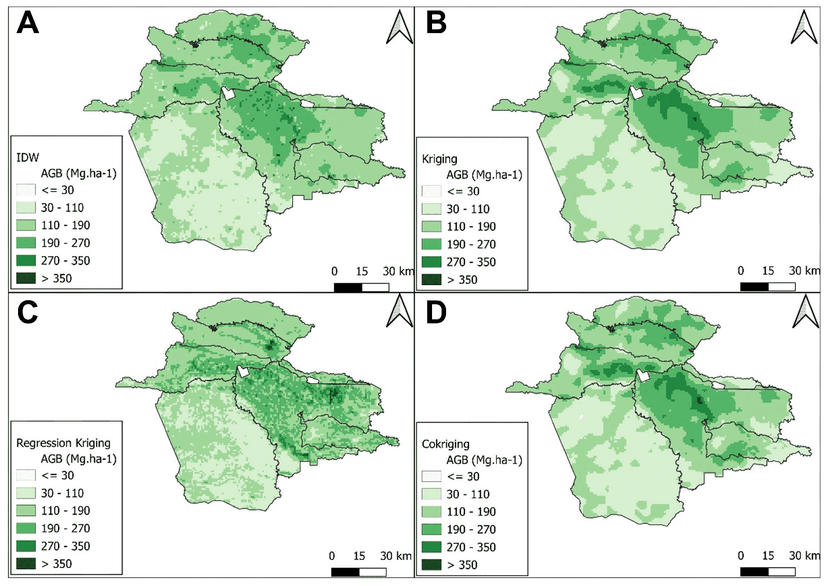
In the test data, however, IDW overestimated AGB predictions, whereas RK showed an extremely low MAE, indicating more accurate predictions (Tab. 2). CK stood out with the lowest RMSE and better overall performance in the test dataset. Considering the RME in interpolated maps, IDW revealed the highest average discrepancy, while RK and CK showed similar RMEs. The interpolation map for each utilized method is presented in Fig. 2.
Fig. 2 - Aboveground biomass (AGB) maps in Mg ha-1 generated by different spatial modeling methods for the Carajás Mosaic.
The total AGB estimated for the original forest areas (1.15 million km2) of the Carajás Mosaic varied from 539.091.30 (obtained using the IDW method) to 540.358.83 Mg (obtained using the RK method - Tab. 4), equivalent to a maximum difference of only 0.235% among the AGB values obtained through different spatial modeling techniques. In addition to satisfactory RME, the correlation between pixels for OK and CK was R2 = 0.99; R2 = 0.61 between RK and OK; R2 = 0.60 between RK and CK. For IDW, there was a correlation of (R2 = 0.82) for both OK and CK, and (R2 = 0.72) with RK.
Tab. 4 - Descriptive statistics (mean, minimum, maximum, standard deviation, and total) of the aboveground biomass (AGB) maps generated by each spatial interpolation method, and carbon stocks calculated using the conversion fraction = 0.47.
| Statistics | Methods | |||
|---|---|---|---|---|
| IDW | Kriging | Regression kriging |
Cokriging | |
| Mean (Mg ha-1) | 148.10 | 148.16 | 148.45 | 148.15 |
| Minimum (Mg ha-1) | 11.31 | 33.64 | 35.84 | 25.98 |
| Maximum (Mg ha-1) | 420.56 | 345.83 | 310.78 | 365.36 |
| Standard Deviation (Mg ha-1) | 61.66 | 62.65 | 52.19 | 64.31 |
| Total AGB (Mg) | 539.091.30 | 539.315.99 | 540.358.83 | 539.291.85 |
| Total Carbon (106 Mg C ha-1) | 80.36 | 80.39 | 80.55 | 80.39 |
Influence of geology on AGB estimates
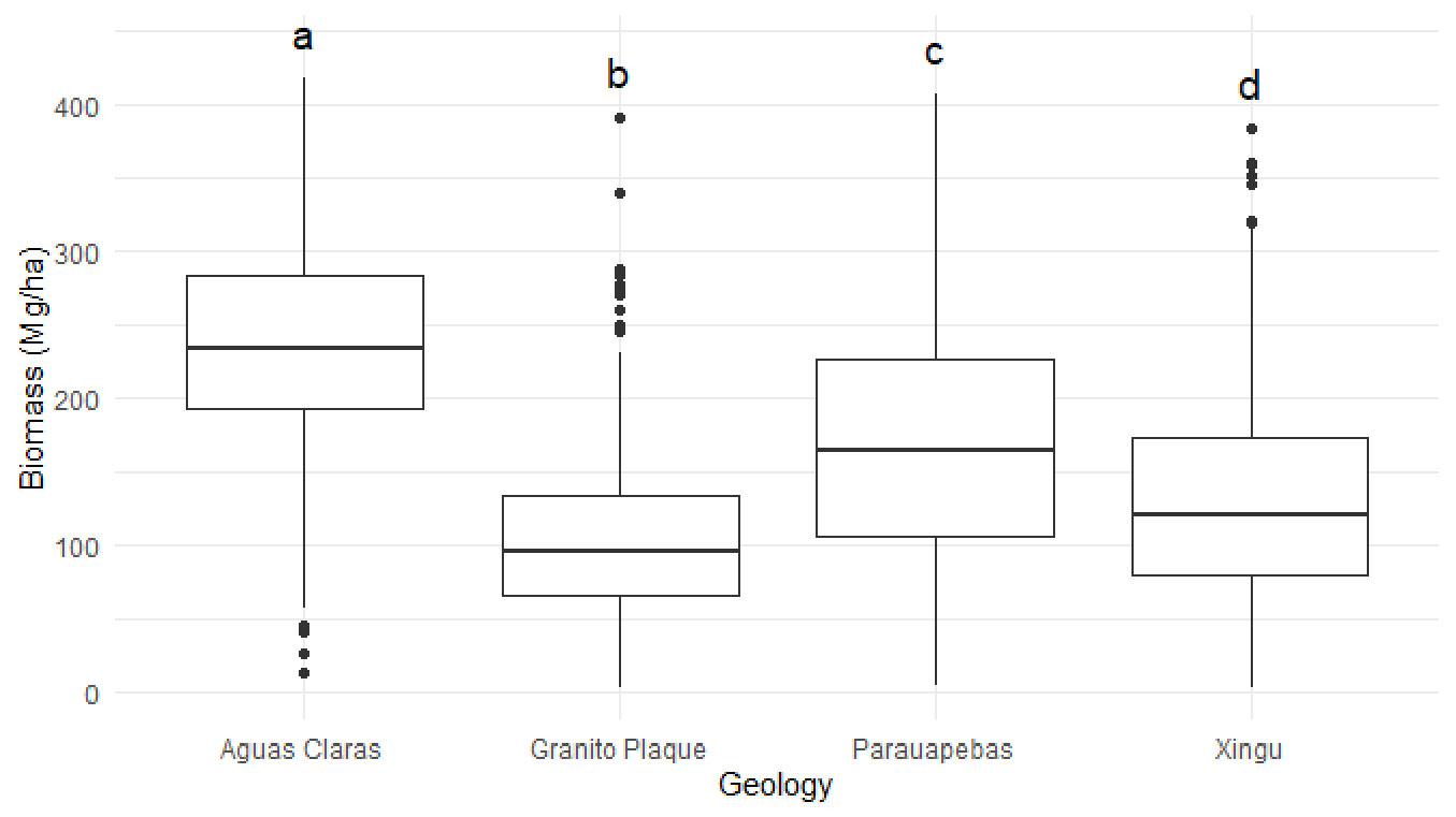
A significant difference in AGB among all geological typologies was detected (χ2 = 1191.3, df = 3, p-value < 2.2e-16 - see Supplementary material). The highest mean AGB was observed in Águas Claras (236.07 Mg ha-1), followed by Parauapebas (169.03 Mg ha-1), Xingu Formation (128.09 Mg ha-1), and Granito regions (104.33 Mg ha-1 - Fig. 3).
Fig. 3 - Box-plot of AGB estimated by GEDI across different geological formations in the Carajás Mosaic.
The analysis of the family of kriging methods and the comparison of mean values across different geological formations revealed that the inclusion of auxiliary variables in the estimates significantly influences the correlations among methods. The cokriging (CK) approach exhibited the best validation metrics and a closer approximation to the actual data estimated by GEDI. Based on these results, CK was employed to analyze aboveground biomass (AGB) estimates across protected areas of the Carajás Mosaic, including conservation units and indigenous lands, as well as the main geological formations present in the region. Notably, protected areas dominated by the Águas Claras geological formation exhibited a higher mean AGB compared to other formations (Tab. 5).
Tab. 5 - Minimum (Min), maximum (Max), and the total aboveground biomass (AGB) for each conservation unit and indigenous land in the Carajás Mosaic, including the dominant geology type obtained from the environmental information database of the Brazilian Institute of Geography and Statistics.
| Protected Area | Min | Max | Total AGB (Mg × 100) |
Mean AGB (Mg ha-1) |
Main Geology Formation |
|---|---|---|---|---|---|
| Tapirapé-aquiri National Forest | 64.3 | 316.0 | 372.487.0 | 189.7 | Xingu |
| Carajás National Forest | 35.8 | 375.5 | 704.789.8 | 181.6 | Águas Claras |
| Itacaiunas National Forest | 64.3 | 316.0 | 245.672.6 | 179.1 | Parauapebas |
| Tapirapé Biological Reserve | 72.7 | 268.6 | 168.666.6 | 171.2 | Xingu |
| National Park of Campos Ferruginosos | 47.4 | 256.8 | 113.308.3 | 142.8 | Águas Claras |
| Igarapé Gelado Environmental Protection Area | 45.4 | 210.8 | 25.573.7 | 114.1 | Xingu |
| Xikirin Indigenous Land | 25.9 | 245.6 | 431.302.2 | 98.9 | Granito Plaquê |
Discussion
AGB variability and geostatistical potential
The variability of AGB within primary forests of the Carajás Mosaic has provided a robust basis for the application of geostatistical methods, and the absence of spatial trends in the data was crucial to prevent biased results and ensure that the variance depended only on the distance (h), assuming the intrinsic hypothesis of stationarity ([19]). This variability stems from a complex interaction of edaphoclimatic factors, water availability, geographical gradients, ecological factors, and natural and anthropogenic disturbances ([36]).
The geological heterogeneity of the study area strongly influences soil properties, nutrient availability, and drainage patterns, which in turn affect forest structure and carbon storage ([18]). Areas underlain by the Águas Claras geology exhibited a higher mean AGB compared to other formations, suggesting a potential link between substrate type and carbon storage capacity.
AGB in tropical forests can exhibit substantial spatial variability even within landscapes where average biomass appears relatively stable ([9]). Local factors such as soil type and topography strongly influence tree size, stem density, and the spatial arrangement of vegetation ([45]). Consequently, while the mean landscape-scale AGB may show limited variation, the distribution of biomass across the landscape is shaped by underlying geological features. Incorporating geological information, therefore, enhances our understanding of these spatial patterns and helps identify regions with higher potential for conservation or carbon sequestration.
The exponential model in isotropic semivariogram modeling
The predominance of the exponential model in fitting the generated semivariograms differs from some results found in the literature. The spherical model is often selected in geostatistical modeling of natural forests and forest stands ([31]) and has shown flexibility in explaining the spatial variability of dendrometric variables, such as biomass ([32]). However, our results corroborate the findings of [38]), who also selected the exponential model to explain the semivariogram of AGB in Brazilian states such as Minas Gerais and Bahia. As mentioned above, the AGB grid is derived from the structural behavior of vegetation. Thus, the shape of the semivariogram and the model used may vary with grid resolution and vegetation heterogeneity.
Generally, the contribution (σ²) in forest spectral data is small due to the homogeneity of reflectance, and the ranges (A) tend to be short because they reflect the size of the most significant elements in the image, in this case, tree canopies ([43]). At the spatial resolution used for the Amazon forest, tree-level detail is not possible. Therefore, the spatial dependence structure indicates that pixels within about 6 km exhibit spatial correlation. Consequently, they are influenced by large-scale environmental factors, such as slope, altitude, and soil. Scolforo et al. ([38]) and Viana et al. ([46]) found even larger ranges, up to 150 km, in the biomass semivariogram for the entire Minas Gerais state, reflecting larger biogeographic contexts, including different biomes.
Subsequently, it was observed that the semivariogram structure exhibited a high nugget effect (τ), indicating that unexplained variations at scales below 1 km are significant, i.e., interpixel variation is high. However, the variogram structure presented well-defined parameters, suggesting that errors did not compromise the detection of spatial behavior.
Methods utilizing auxiliary variables achieved the best performance
Among the interpolation methods employed, IDW produced biased estimates on the validation dataset, exhibiting excessive islands known as “bull’s eyes” and noticeable overestimation. This type of interpolation is appropriate when the variable of interest lacks spatial continuity, which is not the case for the AGB GEDI map.
Interpolation methods that utilized auxiliary variables achieved superior performance in validation statistics and produced visually similar biomass maps. Our results align with those of Reis et al. ([34]), who showed that the RK can capture the spatial distribution of AGB. Scolforo et al. ([38]) selected RK as the best method for spatializing AGB in Minas Gerais, using latitude and altitude as predictor variables. The authors found a Pearson’s correlation of R2 = 0.40, which is very similar to that in our study (R2 = 0.42).
The incorporation of auxiliary variables (slope and SAVI) improved RK performance, yielding residuals and regressed values with spatially balanced, trend-free behavior ([25]). However, the greater dispersion of residuals at higher AGB values can be attributed to several interrelated factors. First, aggregating GEDI footprints into coarser 1-km pixels inherently masks local heterogeneity. This smoothing effect increases uncertainty, particularly in structurally complex, high-biomass areas ([13]). Second, spectral indices derived from optical data, including SAVI, are known to saturate in densely vegetated areas, thereby limiting their sensitivity to variations at very high biomass levels ([27]). Third, slope, though ecologically meaningful, exerts comparatively less influence on biomass in structurally mature and dense forests, where terrain gradients have limited effects on biomass distribution ([36]). Collectively, these factors suggest that the RK model performs reliably across intermediate biomass ranges, while its predictive accuracy decreases for extreme AGB values, as reflected in the increased residual dispersion.
The highest correlation among methods using auxiliary variables showed the greatest similarity, strengthening the reliability of our analyses. The superior performance of these methods may be associated with the use of terrain slope, which helps capture minor variations in AGB distribution across the Carajás Mosaic.
The effect of topography and canopy irregularity on forest AGB estimates
In the Amazon, the spatial variability of forest AGB is influenced by edaphic and topographic characteristics ([5]). In the study area, the slope presented significant variability due to the wide range of landforms. Although SAVI is known to be sensitive to variations in terrain relief ([15]), no significant correlation was found between SAVI and slope within the study area. SAVI is considered a good predictor of AGB in tropical forest areas ([20]), and a negative, even more robust, correlation between AGB and SAVI has been observed in other studies in the Amazon forest ([21]). As forest basal area and AGB increase, so does the amount of shade caused by the irregular structure of the canopy, resulting in a low spectral response in the red band (band 4). As a result, SAVI values decrease, causing a negative correlation with AGB. This circumstance proved advantageous for modeling and was observed in our results. Variations in terrain and vegetation structure contributed to a negative SAVI behavior. According to Roquette ([35]), different forest typologies exhibit distinct characteristics in biomass quantity and distribution patterns. The distribution of AGB is directly linked to the presence of arboreal individuals in vegetation formations, with tree trunks possessing greater carbon storage capacity than roots ([26]).
Literature-based information aligns with our research findings. However, our study relies on indirect measurements obtained from laser and LiDAR data. Consequently, our results are subject to this limitation but can be validated through field data and research. Our final maps serve as a reliable source for a preliminary analysis of estimated AGB in the protected areas of Carajás, employing a consistent and robust statistical approach for interpolation and result validation. As such, the generated products can assist in studies related to conservation, ecology, and forest management in these protected areas.
Conclusions
The estimated AGB for the forests within the Carajás Mosaic exhibited a spatial dependence structure as revealed by the geostatistical semivariogram analysis. Among the tested variables, slope and SAVI were the most effective predictors of variation in AGB density in the region.
Deterministic interpolation poorly performed on the validation dataset, failing to capture the spatial structure of AGB and highlighting the risk of bias and overestimation in sparsely sampled areas.
In contrast, geostatistical interpolation methods provided more consistent and reliable estimates of both AGB and carbon stocks. All three kriging methods demonstrated potential for biomass estimation; however, CK is recommended as it requires only slope as a covariate while still producing accurate results. While OK also yielded robust estimates, its disregard for environmental covariates may limit its ability to capture spatial heterogeneity in AGB across the Amazon. Nonetheless, the selection of a kriging method should be guided by the research objectives, precision requirements, and data availability.
The total estimated AGB for the original forest areas of the Carajás Mosaic was about 539.000 Mg, with minimal variation among the interpolation methods. The highest mean AGB (189.75 Mg ha-1) was observed in the Tapirapé-Aquiri National Forest. Geological formations and terrain features across the protected areas were identified as key environmental drivers of AGB distribution, offering valuable insights for future ecological and carbon stock assessments.
The improved spatial prediction of AGB using slope and SAVI in RK provides a valuable tool for carbon monitoring and conservation planning. The resulting maps allow the identification of high-carbon areas for prioritization, support sustainable management practices, and inform decision-making in REDD+ programs (Reducing Emissions from Deforestation and Forest Degradation, including conservation, sustainable management, and enhancement of forest carbon stocks). These practical applications enhance the relevance of AGB mapping for both ecological assessment and climate change mitigation strategies.
Acknowlegdements
We express our gratitude to the Vale Institute of Technology (VIT) for their initiative on the project “Carbon Emissions and Removal Inventory” by Vale S.A. and for providing research grants for the project (RC100603.IE).
Author’s Contribution
Conceptualization, Methodology, Validation, and Visualization: Souza, RLF; Dionizio, EA; Cavalcante, RBL. Curation, Formal Analysis, and original draft preparation: Souza, RLF. Writing - review and editing: Souza, RLF; Dionizio, EA; Cavalcante, RBL.
References
CrossRef | Gscholar
CrossRef | Gscholar
CrossRef | Gscholar
CrossRef | Gscholar
CrossRef | Gscholar
CrossRef | Gscholar
CrossRef | Gscholar
Gscholar
CrossRef | Gscholar
CrossRef | Gscholar
CrossRef | Gscholar
CrossRef | Gscholar
CrossRef | Gscholar
CrossRef | Gscholar
CrossRef | Gscholar
Online | Gscholar
Authors’ Info
Authors’ Affiliation
Vale Institute of Technology (ITV), Belém, Pará (Brazil)
World Resources Institute (WRI), São Paulo, São Paulo (Brazil)
Vale Institute of Technology (ITV), Belém, Pará (Brazil)
Corresponding author
Paper Info
Citation
Figueiredo De Souza RL, Dionizio EA, Lopes Cavalcante RB (2026). Geostatistical techniques for estimating aboveground biomass in eastern Amazonia. iForest 19: 85-93. - doi: 10.3832/ifor4789-018
Academic Editor
Rafael Da Silveira Bueno
Paper history
Received: Jan 07, 2025
Accepted: Oct 06, 2025
First online: Mar 13, 2026
Publication Date: Apr 30, 2026
Publication Time: 5.27 months
Copyright Information
© SISEF - The Italian Society of Silviculture and Forest Ecology 2026
Open Access
This article is distributed under the terms of the Creative Commons Attribution-Non Commercial 4.0 International (https://creativecommons.org/licenses/by-nc/4.0/), which permits unrestricted use, distribution, and reproduction in any medium, provided you give appropriate credit to the original author(s) and the source, provide a link to the Creative Commons license, and indicate if changes were made.

Web Metrics
Breakdown by View Type
Article Usage
Total Article Views: 1700
(from publication date up to now)
Breakdown by View Type
HTML Page Views: 396
Abstract Page Views: 783
PDF Downloads: 462
Citation/Reference Downloads: 0
XML Downloads: 59
Web Metrics
Days since publication: 94
Overall contacts: 1700
Avg. contacts per week: 126.60
Article Citations
Article citations are based on data periodically collected from the Clarivate Web of Science web site
(last update: Mar 2025)
(No citations were found up to date. Please come back later)
Publication Metrics
by Dimensions ©
Articles citing this article
List of the papers citing this article based on CrossRef Cited-by.
Related Contents
iForest Similar Articles
Review Papers
Remote sensing-supported vegetation parameters for regional climate models: a brief review
vol. 3, pp. 98-101 (online: 15 July 2010)
Review Papers
Accuracy of determining specific parameters of the urban forest using remote sensing
vol. 12, pp. 498-510 (online: 02 December 2019)
Review Papers
Remote sensing of selective logging in tropical forests: current state and future directions
vol. 13, pp. 286-300 (online: 10 July 2020)
Technical Reports
Detecting tree water deficit by very low altitude remote sensing
vol. 10, pp. 215-219 (online: 11 February 2017)
Review Papers
Remote sensing support for post fire forest management
vol. 1, pp. 6-12 (online: 28 February 2008)
Research Articles
Afforestation monitoring through automatic analysis of 36-years Landsat Best Available Composites
vol. 15, pp. 220-228 (online: 12 July 2022)
Research Articles
Assessing water quality by remote sensing in small lakes: the case study of Monticchio lakes in southern Italy
vol. 2, pp. 154-161 (online: 30 July 2009)
Technical Reports
Remote sensing of american maple in alluvial forests: a case study in an island complex of the Loire valley (France)
vol. 13, pp. 409-416 (online: 16 September 2020)
Research Articles
Classification of xeric scrub forest species using machine learning and optical and LiDAR drone data capture
vol. 18, pp. 357-365 (online: 07 December 2025)
Research Articles
Mapping the vegetation and spatial dynamics of Sinharaja tropical rain forest incorporating NASA’s GEDI spaceborne LiDAR data and multispectral satellite images
vol. 18, pp. 45-53 (online: 01 April 2025)
iForest Database Search
Search By Author
Search By Keyword
Google Scholar Search
Citing Articles
Search By Author
Search By Keywords
PubMed Search
Search By Author
Search By Keyword


