Classification of xeric scrub forest species using machine learning and optical and LiDAR drone data capture
iForest - Biogeosciences and Forestry, Volume 18, Issue 6, Pages 357-365 (2025)
doi: https://doi.org/10.3832/ifor4720-018
Published: Dec 07, 2025 - Copyright © 2025 SISEF
Research Articles
Abstract
Arid and semi-arid forest ecosystems represent the largest biomes on Earth. However, research on identifying their species using remote sensing techniques is still limited. Understanding the spatial distribution of vegetation is crucial for precision management. This can be achieved through methods that allow for the individual identification and classification of species, which are essential for accurately estimating forest inventory. The objective of this study was to identify and classify forest species present in a xeric shrubland (arid and semi-arid region) based on multispectral images, red-green-blue (RGB) images, and Light Detection and Ranging (LiDAR) data. All images and data were drone-captured. Machine learning algorithms such as Adaptive boosting (AB), Gradient boosting machine (GBM), Xtreme gradient boosting (XGB), Classification and regression trees (CART), Random Forest (RF), and Support vector machines (SVM) were employed. RF yielded better results for species and shrub class classification, with an accuracy of 0.64 and a Kappa coefficient of 0.56. Classification accuracy values per species were 0.73 (E. antisyphilitica), 0.70 (opuntias), 0.67 (palms), 0.65 (L. tridentata), 0.59 (trees and shrubs), and 0.55 (A. lechuguilla), all of which were obtained by combining the three types of data used. Spectral variables contributed the most metrics, followed by LiDAR and RGB. The results support the adoption of remote drone-mounted sensing systems for characterizing the complex forest vegetation in arid and semi-arid regions, thereby providing a decision-support tool for its management.
Keywords
Arid/semi-arid Ecosystem, Multispectral, Non-timber Forest Management, Remote Sensing
Introduction
Arid and semi-arid forest ecosystems are the largest biomes globally ([5]). Despite that, efforts to demonstrate the capabilities of remote sensing technology, particularly drone-mounted spectral or LiDAR sensors, in identifying and classifying plant species are very scarce worldwide ([32], [25], [26]). Among the main reasons for the limited studies on these ecosystems are their structural complexity and the high diversity of small species. Furthermore, in arid environments, the influence of the soil background on the spectral response can lead to errors such as “same objects with different spectra” or “the same spectrum on different objects”, further complicating the accurate identification of species using remote sensing techniques ([7]). This represents a disadvantage for properly developing forest management plans for such a vast global resource.
Sustainable management of any ecosystem plays a fundamental role in preserving its resources, whether timber or non-timber. To achieve this task, it is necessary to rely on accurate information about the ecosystem structure and composition ([23], [43]). Knowing the different species involved, their current range, and the distribution patterns of individuals allows implementing specialized management for each species based on its growth pattern, spatial arrangement ([9]), and resilience to environmental changes ([34], [27]).
The integration of remote sensing data into a forest vegetation inventory process can result in an efficient and effective classification of tree and shrub individuals of interest, thereby allowing the quantification of the total stock by species in a given area. This is an essential input for sustainable harvest planning of forest raw materials ([42]), and could also result in a significant reduction in the investment required for inventory, particularly in large areas. In contrast, the traditional inventory method, based on field sampling, intensive labor, high costs, and a long execution time ([10]) limits its implementation ([28]).
The recent development in aeronautics allows acquiring affordable drones equipped with miniature high-resolution red-green-blue (RGB), multispectral, hyperspectral, and Light Detection and Ranging (LiDAR) remote sensors that can collect information about land surface features in a considerably shorter time than traditional sensors ([39], [28]). Altogether, these tools effectively describe vegetation in horizontal and vertical dimensions, making them valuable for identifying and classifying plant species across various ecosystems. For instance, accurate species classification has been achieved by combining high-resolution LiDAR and drone-acquired optical data (RGB, multispectral, and hyperspectral). This approach has been successfully applied in grasslands ([21], [36]), xeric shrublands with shrub species ([32], [26], [40]), and forests with tree-like individuals ([34], [28], [43]).
Although drone-based remote sensing data have proven to be valuable, their high spatial resolution implies the generation of large databases ([18]), which, combined with the presence of diverse vegetative structures, creates a complex scenario that demands efficient methods for accurate analysis ([23]).
To address the above challenges, machine learning and deep learning have become essential tools for processing and analyzing such data ([2], [28]). Notable machine-learning algorithms include Gradient Boosting Machines (GBMs), Classification and Regression Trees (CARTs), Random Forests (RFs), and Support Vector Machines (SVMs) ([19], [25], [18]). In deep learning, algorithms such as YOLO, Faster R-CNN, and RetinaNet have shown promising results in species classification based on combinations of RGB, multispectral, hyperspectral, and LiDAR remote sensing data ([1], [11]). Despite these advances, few studies have demonstrated the effectiveness of these technologies in species classification within arid and semi-arid ecosystems. Valuable contributions in this area include the studies by Sankey et al. ([32]), Tang et al. ([35]), Pervin et al. ([26]), Norton et al. ([25]), and Wang et al. ([36]).
This study aimed to identify and classify xeric scrub species from arid and semi-arid regions using a combination of multispectral, RGB, and LiDAR remote sensing data collected by drones. The underlying hypothesis is that the structural variability of a xeric shrubland can be captured in optical and LIDAR variables, thereby enabling the identification of non-timber forest species growing in these ecosystems.
Materials and methods
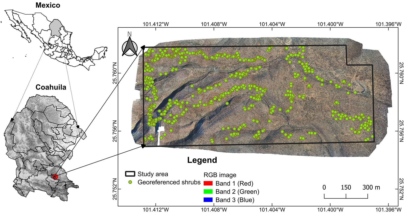
The study area is located within the Ejido Hipólito, Ramos Arizpe Municipality, Coahuila, Mexico (25.756° N, 101.408° W; WGS84 - Fig. 1), covering 116 ha, with altitudes ranging from 1134 to 1249 m a.s.l. and an average slope of 16%. The climate is arid/semi-warm (BSohw), with a precipitation range of 125-300 mm per year and average temperatures of 9-28 °C. The vegetation corresponds to rosetophilous desert scrub under current forest management, dominated by shrubs such as Agave lechuguilla Torr. (Lechuguilla), Euphorbia antisyphilitica Zucc. (Candelilla), Jatropha dioica Cerv. (Sangre de Drago), Larrea tridentata (Sessé & Moc. ex DC.) (Gobernadora), Hechtia glomerata Zucc. (Guapilla), Opuntia spp. (Nopal), and trees such as Vachellia farnesiana (L.) Willd. (Huizache) and Neltuma glandulosa Torr. (Mezquite).
Fig. 1 - Location of the study area. High-resolution RGB image and individual location of shrubland species referenced in the field.
Field data capture and processing
Field surveys were carried out to generate a georeferenced database of 343 plant specimens using a Garmin eTrex® GPS receiver (error ± 3.0 m). Additionally, 303 individuals were identified in the RGB imagery. Sampling was focused on plants with clear and distinctive structures to minimize misidentification with other species. Efforts were made to ensure a homogeneous and spatially dispersed distribution of sampling points across the study area, reflecting species distribution patterns and capturing landscape variability. Overall, the geographic coordinates (latitude and longitude) of 646 individuals were recorded and used for algorithm training (Fig. 1). The GPS coordinates were geometrically corrected to UTM zone 14, WGS84, based on the RGB images.
For the analysis, individual coordinates were organized by species, focusing on the highest-density species: A. lechuguilla (101 specimens), E. antisyphilitica (150), and L. tridentata (92). Additionally, morphologically similar species were grouped into shrub categories, such as opuntias (50 specimens), which included Opuntia rastrera Weber, O. engelmannii subsp. Lindheimeri, Cylindropuntia leptocaulis (DC.) F. M. Knuth, C. imbricata (Haw.) F.M.Knuth; palms (36 specimens), including Yucca filifera Chabaud, Y. treculeana Carrière, Dasylirion cedrosanum Trel.; trees (44 specimens), including V. farnesiana, Senegalia berlandieri Britton & Rose, V. rigidula Benth., N. glandulosa; and shrubs (173 specimens), comprising all remaining species not classified into previous groups.
Remote sensing data and processing
A DJI Phantom 4M multirotor drone flight was conducted, equipped with a five-band multispectral camera: blue (BS, 450 nm), green (GS, 560 nm), red (RS, 650 nm), RedEdge (RE, 730 nm), and near-infrared (NIR, 840 nm). The images were taken at a height of 150 m, with a spatial resolution of 0.10 m, and were georeferenced using an RTK module (Real Time Kinematic) to a UTM zone 14, WGS84 coordinate system (Fig. 2b, Fig. 2f). The orthomosaic, radiometric calibration, and atmospheric correction were all automatically executed in DJI Terra v. 3.8.0.
Fig. 2 - Remotely sensed view of shrub species. LiDAR point cloud (a), multispectral image (b), and RGB image (c). Data acquisition equipment: DJI Matrice 300 RTK with Zenmuse L1 (d) and DJI Phantom 4M (f).
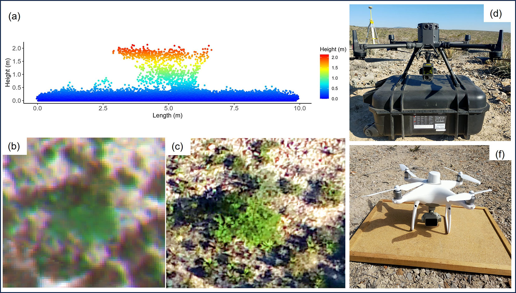
The area was also scrutinized with a DJI Matrice 300 RTK drone, a Zenmuse L1 sensor, and an RGB camera (20 MP - Fig. 2d). The flight altitude was 180 m, with 75% overlap. The RGB images resulted in a spatial resolution of 0.04 m and three bands (red [Rrgb], green [Grgb], and blue [Brgb]), from which hue values were obtained (Fig. 2c). The LiDAR point cloud consisted of two returns and an average density of 193.62 points m-2 (Fig. 2a). Both items were orthorectified by RTK to the UTM zone 14 coordinate system, WGS84. The drone-captured data were processed in RStudio ([29]), using the procedures and methods implemented in the “lidR” packages ([30]) for LiDAR and in the “GLCMTextures” ([8]) package for the extraction of spectral-texture and RGB metrics.
LiDAR-based individual bush extraction
To detect shrubby individuals, the LiDAR point cloud was pre-processed as follows: (i) extreme points (outside the frequency distribution of the maximum and minimum altitudes of the study area) were eliminated by means of altitude filtering (Fig. S1a in Supplementary material); (ii) points were classified into ground and non-ground (vegetation) through the Progressive Morphological Filtering (PMF) procedure ([41]) using a window size of 0.9 m and a height threshold of 0.03 m, which corresponds to the minimum height of existing vegetation (Fig. S1b); (iii) a 0.5 m spatial resolution Digital Elevation Model (DEM) was generated from points classified as ground using the K-nearest neighbor (K-NN) and the Inverse Distance Weighting (IDW) interpolation algorithms; and (iv) the point cloud was normalized by subtracting the DEM to the Z-coordinate (altitude) of each point classified as non-ground. This eliminates the influence of DEM on shrub height ([33] - Fig. S1c).
A 1.5 m-diameter circular sampling window and a minimum cut-off height of 0.05 m were used to detect the highest points corresponding to each shrub in the zone using the normalized cloud and the Local Maximum Filter (LMF) algorithm ([23], [28]). The point cloud was then segmented using the Dalponte2016 algorithm ([3]). This algorithm used the LMF parameters to group and assign a unique identifier to the points that make up each individually segmented shrub. This allowed to accurately measure each shrub in the field and simplify the calculation of height and intensity metrics.
Extraction and selection of optic and LiDAR metrics
To represent the variability of structures and conditions of arid and semi-arid vegetation, 143 metrics were calculated from LiDAR (57), spectral (54), and RGB (32) data. The latter include the BS, GS, RS, RE, and NIR spectral (S) bands, and the color levels (RGB = 0-255) Rrgb, Grgb, and Brgb. To reduce the effect of saturation on image values, eight texture metrics per band were included, derived from the Gray Level Co-occurrence Matrix (GLCM), which are: mean (Me), variance (Va), correlation (Co), entropy (En), second moment (Sm), homogeneity (Ho), contrast (Con) and dissimilarity (Di) ([8]).
Additionally, 14 vegetation indices (VIs) were included to mitigate the effect of soil albedo on vegetation reflectance and to highlight variations across different cover types. The NDVI, RVI, DVI, SAVI, MSAVI, GCI, GDVI, GRVI, and GNDVI indices were generated from spectral data, and the GRVI, RGBVI, GLI, VARI, and NGRDI indices from RGB images ([24], [6], [12], [28] - see Tab. S1 in Supplementary material).
The LiDAR metrics were extracted from the normalized segmented cloud to use the specific records of each detected individual. For this, the normalized Z attributes (Height, m - [33]), the intensity, and the classification of points ([2]) were used. The extraction was performed by deriving standard metrics at different levels of regularization using the “stdmetrics” function in the “lidR” package ([22], Tab. 1). The altitude (m) of each individual was also obtained from the LiDAR-generated DEM.
Tab. 1 - List of vegetation structure metrics calculated from the segmented LiDAR point cloud for each detected shrub individual.
| Attribute | Code | Description | Attribute | Code | Description |
|---|---|---|---|---|---|
| Point cloud | n | Number of points | Intensity | itot | Sum of intensities for each return |
| area | Individual area (m2) | imax | Maximum intensity | ||
| Normalized Z | zmax | Maximum height (m) | imean | Mean intensity | |
| zmean | Mean height (m) | isd | Standard deviation of intensity | ||
| zsd | Standard deviation of height | iskew | Skewness of intensity | ||
| zskew | Skewness of height | ikurt | Kurtosis of intensity | ||
| zkurt | Kurtosis of height | ipground | Intensity returned by points classified as "ground" (%) | ||
| zentropy | Entropy of height | ipcmzqx | Intensity returned below the k-percentile of height (%) | ||
| pzabovezmean | returns above zmean (%) | ipxth | Intensity returned by 1st, 2nd, 3rd,xth, returns (%) | ||
| pzabovex | Returns above the x percentile (%) | Point cloud | n | Number of points | |
| zqx | Quantile of height | area | Individual area (m2) | ||
| zpcumx | Cumulative returns per individual (%) | Classification | pground | Returns classified as "ground" (%) |
Including diverse variables in the modeling process can lead to redundant information, thus affecting classification accuracy ([2]). To avoid redundancy, we used the Random Forests with Boruta (RFB) and the Xtreme Gradient Boosting (XGB) algorithms to select relevant variables. RFB uses random permutations to choose variables that significantly (α=0.05) contribute to an increased accuracy ([17]). XGB evaluates the increase in node purity using the Gini coefficient, which serves as a unit of measurement for estimating prediction variance ([14]). In both cases, variables with a positive and significant importance value were selected.
Statistical analysis
Six machine learning algorithms were evaluated to classify shrub individuals. All algorithms were adjusted using ensemble models to increase accuracy. Boosting was used for AdaBoost (adaptive boosting, AB), GBM, and XGB; Bagging for CART, RF, and SVM. In the latter, a Gaussian Kernel was used to achieve appropriate adjustments when working with a high number of variables ([15]). Optimal hyperparameters for the models were determined via cross-validation with 5 to 10 iterations. All algorithms were performed in the RStudio “caret” package ([16]).
The algorithms were trained and evaluated in two phases. First, the models were adjusted with two selection approaches (RFB and XGB) and with all the variables generated from the spectral data, RGB, and LiDAR; for both selection approaches, the best algorithms, as well as the set of variables (metrics) with the most significant contribution to the classification, were selected. In the second phase, the algorithms with the best statistics were adjusted using the chosen set of variables to evaluate the capacity of the different types of data, used individually and combined, to classify shrub vegetation in arid and semi-arid ecosystems.
Seventy percent of the field data was used to train the algorithms, and the remaining 30% was used as a test set. The models’ fit was assessed using bias and agreement measures derived from each algorithm’s confusion matrix: overall training accuracy (TA), overall test accuracy (OTA), the Kappa coefficient (K), and specific accuracy per classification group (SA). In addition, the importance of the variables in the classification was assessed with the Gini coefficient ([14]).
Results
Individual bush segmentation
The identification of individuals derived from the LiDAR cloud revealed a total of 471.625 shrubs of all species associated with xerophytic scrub in the study area. These presented an average individual shrub cover of 0.232 m2 (range: 0.0094-12.223 m2) and an average height of 0.342 m (range: 0.05-6.63 m). The individuals’ geographic locations showed an average spatial error of 0.40 m relative to the multispectral image, attributable to differences in acquisition equipment. This mismatch was rectified by a geometric correction of the multispectral image from the RGB orthomosaic (see Fig. S2 in Supplementary material).
Selection of metrics and algorithm evaluation
The 143 spectral, RGB, and LiDAR metrics were extracted for each individual detected in the point cloud (471.625 shrubs) and for the sampled individuals (646 shrubs). Five metrics related to the percentage of return intensity (ipxth) were excluded because they lacked values, leaving 138 metrics. The selection of variables with RFB was reduced to 102 metrics (LiDAR: 35, spectral: 43, and RGB: 24), whereas XGB selected only 32 (LiDAR: 13, spectral: 12, and RGB: 7). Regarding the efficiency of the variable sets, RFB (TA: 0.70, OTA: 0.55, K: 0.64) and without selection (TA: 0.70, OTA: 0.54, K: 0.63) presented the highest accuracy. In contrast, XGB had lower accuracy (TA: 0.67, OTA: 0.55, K: 0.61), due to its strict discrimination, which could eliminate essential variables for a specific class of shrubs (Fig. 3).
Fig. 3 - Accuracy of algorithms and variable selection methods for the classification of xerophytic shrub species. (TA): overall training accuracy; (OTA): overall test accuracy; (K): Kappa coefficient; (AB): adaptive boosting; (GBM): gradient boosting machine; (XGB): Xtreme gradient boosting; (CART): classification and regression trees; (RF): Random Forest; (SVM): support vector machines.
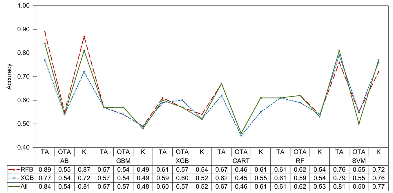
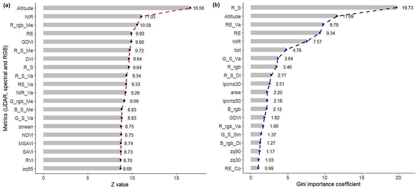
Of the selected variables, the most relevant in the classification of shrubs were Altitude, NIR, Rrgb_Me, RE, and GDVI, for the RFB method (Fig. 4a); and RS, Altitude, RE_Va, RE, NIR, and itot with XGB (Fig. 4b). In general, spectral and RGB images presented a greater number of variables with significance in both methods, in addition to their texture and VI derivatives. For LiDAR, the reduction was greater, which implies a lesser contribution (Fig. 4). With these sets of variables (RFB, XGB, and without selection), the AB, GBM, XGB, CART, RF, and SVM algorithms were evaluated, in which the overall mean TA was 0.69, OTA was 0.54, and K was 0.63. The highest values of TA and K were presented in AB (0.83 and 0.80, respectively), SVM (0.79 and 0.75), and CART (0.65 and 0.59); whereas the lowest were in GBM (0.57 and 0.49 - Fig. 3).
Fig. 4 - Selected spectral, RGB, and LiDAR metrics with (a) Random Forests with Boruta (RFB), and (b) extreme gradient boost (XGB) with greater significance in the classification of xerophytic shrubland species. (R): red; (G): green; (B): blue; (S): spectral data; (rgb): RGB data; (Me): mean; (Va): variance; (Di): dissimilarity; (Sm): second moment.
As for OTA, the best models were RF (0.61), XGB (0.58), and GBM (0.55), whereas the rest showed a drop in OTA relative to TA, suggesting overfitting and the inability to predict new observations accurately. In this parameter, CART (0.46) had the lowest fit (Fig. 3). The algorithms that performed best in bush classification were AB, SVM, and RF. The first two were chosen for their ability to fit the training data, while the last one stood out for its statistical stability and higher prediction accuracy (OTA). Using these three best-fitting algorithms and the set of metrics generated with RFB, which was superior, the remote sensing data types were evaluated for species and shrub class classification.
Spectral, RGB, and LiDAR data assessment
Across all data combinations, the AB and SVM algorithms achieved the highest average training accuracy (TA: 0.74 and 0.68, K: 0.69 and 0.62, respectively). However, prediction in the OTA is low (0.44 and 0.46) (Tab. 2), which means overfitting and a low efficiency to perform new estimations. On the contrary, although RF obtained lower training values for TA and K, its accuracy was higher in the test set (OTA: 0.49), in addition to show stability in the learning and prediction process (Tab. 2). Therefore, the RF model was selected for the assessment of LiDAR, spectral, and RGB data.
Tab. 2 - Accuracy of the three selected models using spectral, RGB, and LiDAR data individually and combined for the classification of species and shrub groups of a xeric shrubland. (RFB): Random forests with Boruta; (AB): Adaptive boosting; (RF): Random forests; (SVM): Support vector machines; (TA): overall training accuracy; (OTA): overall test accuracy; (K): Kappa coefficient; (L): LiDAR; (S): spectral; (RGB): red-green-blue image.
| Selection | Data | AB | RF | SVM | ||||||
|---|---|---|---|---|---|---|---|---|---|---|
| TA | OTA | K | TA | OTA | K | TA | OTA | K | ||
| RFB | L | 0.67 | 0.34 | 0.61 | 0.42 | 0.33 | 0.32 | 0.58 | 0.35 | 0.49 |
| S | 0.63 | 0.39 | 0.55 | 0.47 | 0.43 | 0.37 | 0.65 | 0.42 | 0.58 | |
| RGB | 0.67 | 0.39 | 0.60 | 0.42 | 0.42 | 0.30 | 0.61 | 0.40 | 0.53 | |
| L-S | 0.74 | 0.45 | 0.69 | 0.54 | 0.52 | 0.45 | 0.70 | 0.51 | 0.64 | |
| L-RGB | 0.78 | 0.43 | 0.74 | 0.53 | 0.49 | 0.43 | 0.68 | 0.49 | 0.62 | |
| S-RGB | 0.79 | 0.45 | 0.75 | 0.51 | 0.51 | 0.42 | 0.70 | 0.51 | 0.65 | |
| L-S-RGB | 0.89 | 0.55 | 0.87 | 0.61 | 0.62 | 0.54 | 0.76 | 0.55 | 0.72 | |
| - | Mean | 0.74 | 0.44 | 0.69 | 0.51 | 0.49 | 0.42 | 0.68 | 0.46 | 0.62 |
When the predictive power (OTA) of different types of remote sensing data for shrub species classification was compared, spectral data showed the highest accuracy (0.43), followed by RGB (0.42) and LiDAR metrics (0.33). The combination of two types of data increased the classification accuracy in all cases (Tab. 2). The data set composed of LiDAR and spectral data was superior (0.52), with an increase of 20.93%, 23.81% and 57.58% compared to the independent use of spectral, RGB, and LiDAR variables, respectively. Finally, combining all three data types (0.62) yielded an accuracy gain of 19.23%, suggesting that using all variables together improves the classification of species and shrub classes.
Classification of shrub species and classes
The RF algorithm was trained to classify shrub species and groups using 646 individuals and a combination of three types of selected and refined remote sensing data. The overall accuracy was 0.64 (range: 0.60-0.68), and the Kappa index was 0.56. The minimum specific accuracy (SA) achieved for the classes was 0.55. The values for each species and shrub group were 0.73 (E. antisyphilitica), 0.70 (opuntias), 0.67 (palms), 0.65 (L. tridentata), 0.59 (trees and shrubs), and 0.55 (A. lechuguilla).
Spectral data made a greater contribution to species and shrub group classification, as they provided more variables. Among the 20 variables with the highest importance, spectral data contributed with 10 metrics to the shrub classification (NIR, DVI, RS, RE, GDVI, SAVI, NIR_Va, MSAVI, GS, BS), compared to eight metrics extracted from LiDAR (Altitude, zmean, zq95, zq85, zmax, zq65, zsd, zq80) and two metrics from the RGB image (Rrgb_Me, Grgb_Me - Fig. S3 in Supplementary material). Of all metrics, altitude made the most significant contribution, followed by a group of spectral variables (bands and VI NIR, DVI, RS, RE, GDVI). Texture metrics from RGB data had less influence on species discrimination.
The results of the classification of the 471.625 shrubs detected with LiDAR are shown in Tab. 3. Adequate classifications were obtained for E. antisyphilitica and L. tridentata, as well as for the group of trees, opuntias, and palms. Field density and spatial distribution were obtained according to model estimates (Fig. 5). However, a low precision was observed when classifying A. lechuguilla (one of the most abundant species in the study area), despite having a good number of samples for fitting the model, so an underestimation of this species is assumed. This may be because the spectral response of A. lechuguilla could have been confused with that of other species in the shrub class. In fact, distinguishing it from similar species can be difficult due to its agglomerated growth form ([31], [25]).
Tab. 3 - Classification parameters of shrubs detected with the LiDAR point cloud in the study area and average dimensionality values.
| Species/Category | Training Individuals (n) |
Classified individuals (n) |
Classified individuals (%) |
Mean height (m) |
Mean coverage (m2) |
|---|---|---|---|---|---|
| A. lechuguilla | 101 | 46.272 | 9.8 | 0.265 | 0.229 |
| Trees | 44 | 1.897 | 0.4 | 1.183 | 0.530 |
| Shrubs | 173 | 251.161 | 53.3 | 0.334 | 0.230 |
| E. antisyphilitica | 150 | 120.404 | 25.5 | 0.271 | 0.230 |
| L. tridentata | 92 | 43.693 | 9.3 | 0.549 | 0.229 |
| Opuntias | 50 | 5.326 | 1.1 | 0.542 | 0.231 |
| Palms | 36 | 2.872 | 0.6 | 1.091 | 0.425 |
Fig. 5 - Classification of individuals by shrub species and groups of a xerophytic shrubland obtained from remote sensing data and the Random Forest model.
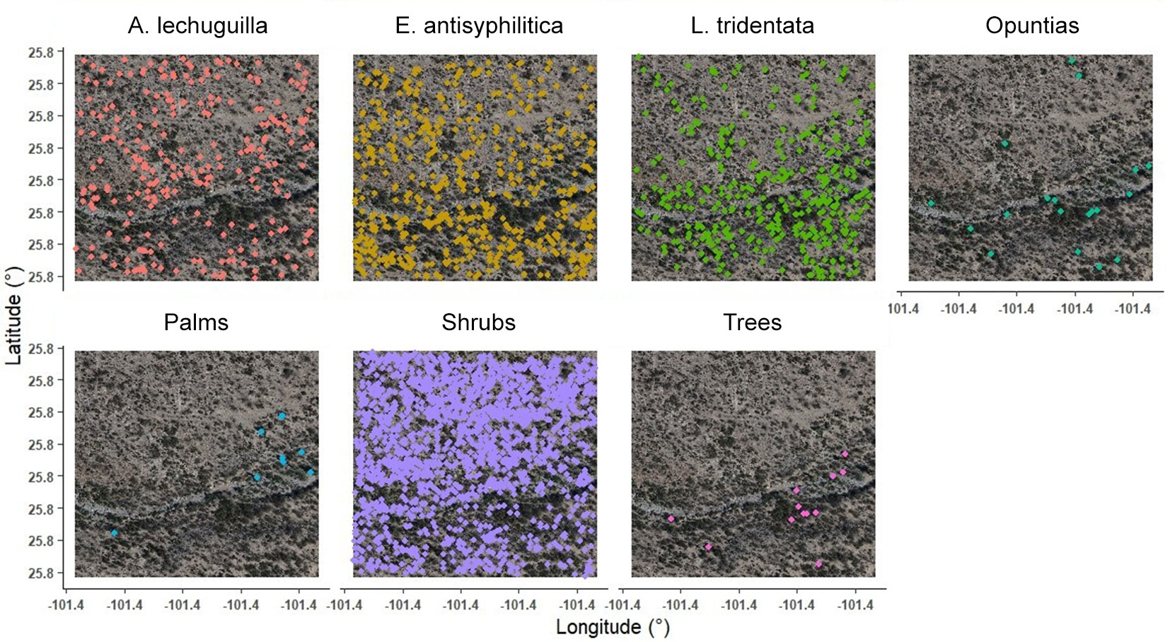
The classified species and groups presented coverages of 0.557 m2 for trees, 0.231 m2 for shrubs, 0.230 m2 for opuntias, 0.408 m2 for palms, 0.230 m2 for E. antisyphilitica, 0.228 m2 for L. tridentata, and 0.229 m2 for A. lechuguilla. The highest height was registered in the tree group (1.18 m, range; 0.30-5.13 m), followed by the palms (1.09 m, range: 0.32-4.50 m), whereas the rest were distributed between average heights ranging from 0.25 m to 0.55 m (Tab. 3). Regarding this variable, overestimates were found in all classes, especially for E. antisyphilitica and A. lechuguilla with maximum heights of 4.81 m and 4.03 m, respectively, values that are outside the expected growth interval of these species.
Discussion
Individual shrub segmentation
In this study, LiDAR data and the FML algorithm were used to segment individual plants based on vegetation structural dimensions, yielding accurate results validated against RGB images (Fig. S2 in Supplementary material). These findings are consistent with recent studies on individual tree detection ([37], [23], [28]), although with lower accuracy for shrubs. This reduced accuracy is attributed to the morphological diversity of vegetation in arid and semi-arid ecosystems, which includes spherical, cylindrical, and rectangular shapes ([20]). Furthermore, in areas with high species density, both underestimation of individual counts and overestimation (false individuals) in bare soil areas associated with rocky bodies were observed.
The bias generated in the detection of individuals is attributed to the similarity in the vegetation height. This was observed during maximum Z-value filtering, where only larger individuals were identified, and the smaller ones were eliminated, making it difficult to separate individual shrubs and leading to individual loss during LiDAR scanning. Sankey et al. ([31]) mentioned that accuracy in this process is highly dependent on the quality of cloud segmentation, which is influenced by point density, number of bounces, structural similarity, and species agglomeration. In addition, using fixed parameters to identify all species or plant strata can increase detection errors, particularly for shrub species ([4]).
Using vegetation-based parameters improved the detection of individuals. This is supported by recent findings of Wu et al. ([37]) and Xu et al. ([38]), who used small windows and a minimum cut-off height to generate a higher number of individuals in shrub or small vegetation. In particular, the cut-off height is crucial for detecting individuals. It should be comparable to the minimum vegetation height to capture the variability in shrub and tree structures ([26]). In addition, it is recommended to adopt a short cut-off height, according to the flattened shape of the shrub canopy, as described by Qian et al. ([27]).
Selection of metrics and algorithm evaluation
A crucial step in the training process is variable selection, which helps eliminate multicollinearity and less important variables, thereby improving the accuracy and performance of algorithms in classification and regression ([18]). In this study, 138 remotely sensed metrics were employed to characterize three species and seven shrub groups in a xerophytic rosetophytic shrubland. Two variable selection techniques were applied, RFB and XGB, which reduced the metrics by 26.10% and 76.81%. The first was selected to avoid omitting important information during classification. This is also recommended for modeling complex structures, such as vegetation in arid and semi-arid ecosystems, where a large set of variables is needed to achieve species discrimination with low estimation bias ([2], [18]). In addition, several studies highlight the integration of remote sensing data to improve classification accuracy and detail ([25], [36]). In this case, precision increased by 3.3% by eliminating correlated or redundant variables. This improvement has been corroborated in similar studies, which demonstrated that optimal variable selection can improve the accuracy of species classification. This finding applies to both shrubby species in arid and semi-arid regions ([39], [25], [26], [35]) and arboreal species in temperate and tropical forests ([4], [18]).
Evaluation of spectral, RGB, and LiDAR data
The effectiveness of integrating data from multiple remote sensors for classifying plant species across various ecosystems has already been documented. The best results have been obtained by combining metrics derived from LiDAR and optical imaging (spectral and RGB - [25], [43], [18]). In this work, integrating optical and LiDAR remote sensing data increased the classification accuracy of shrub species by 23.80%, with OTA rising from 0.42 when used individually to 0.52 when combining the three data types, which aligns with previous findings. As reported by Qian et al. ([27]) the inclusion of vegetation structure metrics (LiDAR) improves the estimates by describing the dimensions of plant species and by complementing the optical information for a complete characterization of vegetation ([2], [43]). The individual use of these data limits the ability to describe vegetation properties, as variables are captured separately along a single dimension ([28], [18]). Therefore, it is necessary to incorporate various types of remotely sensed data to achieve a comprehensive characterization of vegetation, covering both its vertical and horizontal aspects.
Data derived from multispectral images yielded the best results, which agree with similar research on classifying shrubby individuals from other arid and semi-arid regions ([31], [32], [23], [28]). This is because the spectral signatures of the species can be discriminated, along with the high spatial resolution of the spectral and RGB images (0.10 m). Although LiDAR did not perform well in species classification, it was indispensable for improving the results.
Nonetheless, this result differs from the findings reported by Liu et al. ([19]) and Cao et al. ([2]), who observed better performance with LiDAR metrics than with optical data. This can be attributed to the fact that these authors modelled the tree structures of coniferous forests, in which the crown spectral response is similar, and the most relevant differences lie in the arrangement of branches and crown morphometry, aspects better represented by structure-derived LiDAR variables. Moreover, Zhong et al. ([43]) noted that differences in the efficiency of different types of remote sensing data are attributable to the capture season and sensor type, as well as to the complexity of the evaluated phenomenon and the classification algorithm used.
Classification of shrub species and classes
Our results align with similar studies that used the RF machine learning algorithm to classify shrub species in arid and semi-arid regions. Although RF did not achieve the highest training accuracy, it demonstrated superior prediction performance compared to the SVM and AB algorithms ([2], [25], [28]). These results align with other studies that compare several classification algorithms, showing that RF achieves higher prediction accuracy than SVM, AB, CART, and GBM ([19], [18]). This success is attributed to RF’s flexible nature as a learning algorithm, especially its ability to effectively handle large datasets ([13]). RF divides the data into adaptive sections (i.e., trees), and fits a model specifically for each classification group. This adaptive approach has proven fundamental for obtaining accurate results ([32], [26]). In contrast, Mayra et al. ([23]) showed that, when classifying tree species in a mixed temperate forest, decision tree-based methods (GBM and RF) had significant difficulties in separating deciduous species, which was attributed to the spatial incompatibility of field and remotely sensed data, affecting the spectral signature of species.
On the other hand, classification accuracies in this study ranged from 0.55 to 0.73 at the species level, and an overall accuracy of 0.64. The accuracy levels may have been influenced by factors such as the amount of data available per species and shrub class, as well as the distinct characteristics of each species. Additionally, the species density imbalance in the study area could have contributed to these results. In this regard, Huang et al. ([11]) demonstrated that classification accuracy in arid grasslands varied with sample size per class, reporting accuracies of 0.78-0.90, which are higher than those found in this study. Similarly, Norton et al. ([25]) achieved accuracies of 0.86-0.98 when classifying five tree species in semi-arid ecosystems, while Liu et al. ([20]) obtained accuracies of 0.70-0.82 using a combination of remote sensing data (LiDAR, multispectral, and RGB) to improve classification precision.
Although these technologies offer promising advances in species classification and environmental monitoring, they still face significant challenges, including issues with data quality and ongoing improvement needs. Addressing these limitations is critical to fully realizing the potential of drone-borne remote sensing in non-timber forest management.
Conclusions
This study demonstrates the potential of combining high-resolution multispectral, RGB, and LiDAR data acquired with drone-borne sensors with machine learning algorithms for classifying xeric scrub vegetation in arid and semi-arid ecosystems. Combining LiDAR structural information with optical data (multispectral and RGB), the proposed approach achieved a 19.23% improvement in classification accuracy compared to the individual data sources. This multidimensional strategy enabled not only the detection and spatial mapping of over 471.625 individual shrubs using LiDAR point clouds, but also the successful identification of non-timber forest species with moderate to high accuracy. The results emphasize the relevance of spectral variables in distinguishing among species and highlight the critical role of LiDAR in capturing vegetation structure, particularly vertical complexity.
These findings highlight the value of drone-based remote sensing combined with machine learning algorithms as a novel, scalable, and cost-effective framework for precision forest management in data-scarce arid and semi-arid ecosystems.
Future applications of this approach may include monitoring vegetation dynamics, assessing biodiversity, and informing restoration strategies, thereby contributing to the sustainable management of dryland forest resources.
Acknowledgments
The first author thanks the Secretaría de Ciencia, Humanidades, Tecnología e Innovación (SECIHTI) for the scholarship granted to pursue his doctoral studies in Forest Sciences at the Colegio de Postgraduados. We would also like to thank the Instituto Nacional de Investigaciones Forestales, Agrícolas y Pecuarias (INIFAP) for funding the project “Estimation of forest variables in arid and semi-arid ecosystems using remote sensing data for the use of non-timber forest resources”, through which the field data were collected.
Conflicts of Interest
The authors declare no conflict of interest.
References
CrossRef | Gscholar
CrossRef | Gscholar
CrossRef | Gscholar
Gscholar
Gscholar
CrossRef | Gscholar
CrossRef | Gscholar
CrossRef | Gscholar
Authors’ Info
Authors’ Affiliation
José René Valdez-Lazalde 0000-0003-1888-6914
Héctor Manuel De Los Santos-Posadas 0000-0003-4076-5043
Valentín José Reyes-Hernández 0000-0002-1804-412x
Postgrado en Ciencias Forestales, Colegio de Postgraduados, Campus Montecillo (México)
Antonio Cano-Pineda 0000-0003-4924-8050
Instituto Nacional de Investigaciones Forestales, Agrícolas y Pecuarias - INIFAP, Campo Experimental Saltillo, Saltillo, Coahuila (México)
Instituto de Silvicultura e Industria de la Madera, Universidad Juárez del Estado de Durango, Durango (México)
Postgrado en Hidrociencias, Colegio de Postgraduados Campus Montecillo (México)
Corresponding author
Paper Info
Citation
Hernández-Ramos A, Valdez-Lazalde JR, De Los Santos-Posadas HM, Reyes-Hernández VJ, López-Serrano PM, Cano-Pineda A, Flores-Magdaleno H (2025). Classification of xeric scrub forest species using machine learning and optical and LiDAR drone data capture. iForest 18: 357-365. - doi: 10.3832/ifor4720-018
Academic Editor
Francesco Ripullone
Paper history
Received: Sep 05, 2024
Accepted: Sep 14, 2025
First online: Dec 07, 2025
Publication Date: Dec 31, 2025
Publication Time: 2.80 months
Copyright Information
© SISEF - The Italian Society of Silviculture and Forest Ecology 2025
Open Access
This article is distributed under the terms of the Creative Commons Attribution-Non Commercial 4.0 International (https://creativecommons.org/licenses/by-nc/4.0/), which permits unrestricted use, distribution, and reproduction in any medium, provided you give appropriate credit to the original author(s) and the source, provide a link to the Creative Commons license, and indicate if changes were made.

Web Metrics
Breakdown by View Type
Article Usage
Total Article Views: 3890
(from publication date up to now)
Breakdown by View Type
HTML Page Views: 1524
Abstract Page Views: 1528
PDF Downloads: 732
Citation/Reference Downloads: 0
XML Downloads: 106
Web Metrics
Days since publication: 189
Overall contacts: 3890
Avg. contacts per week: 144.07
Article Citations
Article citations are based on data periodically collected from the Clarivate Web of Science web site
(last update: Mar 2025)
(No citations were found up to date. Please come back later)
Publication Metrics
by Dimensions ©
Articles citing this article
List of the papers citing this article based on CrossRef Cited-by.
Related Contents
iForest Similar Articles
Review Papers
Remote sensing-supported vegetation parameters for regional climate models: a brief review
vol. 3, pp. 98-101 (online: 15 July 2010)
Review Papers
Accuracy of determining specific parameters of the urban forest using remote sensing
vol. 12, pp. 498-510 (online: 02 December 2019)
Review Papers
Remote sensing of selective logging in tropical forests: current state and future directions
vol. 13, pp. 286-300 (online: 10 July 2020)
Technical Reports
Detecting tree water deficit by very low altitude remote sensing
vol. 10, pp. 215-219 (online: 11 February 2017)
Review Papers
Remote sensing support for post fire forest management
vol. 1, pp. 6-12 (online: 28 February 2008)
Research Articles
Mapping the vegetation and spatial dynamics of Sinharaja tropical rain forest incorporating NASA’s GEDI spaceborne LiDAR data and multispectral satellite images
vol. 18, pp. 45-53 (online: 01 April 2025)
Technical Reports
Remote sensing of american maple in alluvial forests: a case study in an island complex of the Loire valley (France)
vol. 13, pp. 409-416 (online: 16 September 2020)
Research Articles
Afforestation monitoring through automatic analysis of 36-years Landsat Best Available Composites
vol. 15, pp. 220-228 (online: 12 July 2022)
Research Articles
Geostatistical techniques for estimating aboveground biomass in eastern Amazonia
vol. 19, pp. 85-93 (online: 13 March 2026)
Research Articles
Assessing water quality by remote sensing in small lakes: the case study of Monticchio lakes in southern Italy
vol. 2, pp. 154-161 (online: 30 July 2009)
iForest Database Search
Google Scholar Search
Citing Articles
Search By Author
- A Hernández-Ramos
- JR Valdez-Lazalde
- HM De Los Santos-Posadas
- VJ Reyes-Hernández
- PM López-Serrano
- A Cano-Pineda
- H Flores-Magdaleno
Search By Keywords


