A new zoning index for detecting areas of biological importance applied to a temperate forest in Central Mexico
iForest - Biogeosciences and Forestry, Volume 16, Issue 4, Pages 253-261 (2023)
doi: https://doi.org/10.3832/ifor4111-016
Published: Aug 31, 2023 - Copyright © 2023 SISEF
Research Articles
Abstract
Biodiversity conservation is a priority because it is the cornerstone of ecosystem services and natural cycles, providing essential resources for the development of humans and other species. Several indices have been proposed to prioritize areas needing protection. However, some require specific information while others are based on subjective categorical variables, are limited to a particular plant community or cannot be represented at a spatial scale. We developed an Index of Importance for Biological Conservation (InICoB), which was applied to a temperate forest in central Mexico but can be used for any plant community by adjusting some of its parameters. The proposed index is objective, based on quantitative indicators of vegetation composition and structure, and can be spatially projected. InICoB was tested and validated on a temperate cloud forest (CF) and its associated communities: advanced secondary vegetation (ASV) / coffee plantations (CP), agriculture, and induced grasslands. Life forms, presence of endemic, climax, native and protected species, diversity, structural complexity, and complementarity were used as indicators in its construction. InICoB was calculated for 63 sampling units (SUs), and a geostatistical model was incorporated for its interpolation with environmental and social variables as predictors. The results show that InICoB adequately evaluated the different environmental units that cover the locality. Significant differences were observed between the forest and the secondary/induced vegetation. The highest value of InICoB (0.91) was found in the CF, and the lowest in induced vegetation (0.3). The geostatistical model showed that occupation of the land, distance to town, and slope have an important influence on InICoB. The advantages of InICoB include the use of quantitative indicators that can be applied to any plant community. Additionally, it is flexible with respect to the data collected, it can be calculated only with the presence/absence of species or it can include forest measurement data. Furthermore, it is easy to interpret and can be spatially represented in a raster layer that can be added to a geographic information system. Therefore, it can be a very helpful tool in decision-making for land use planning and evaluation of the effects of human activities on plant communities.
Keywords
Biodiversity Conservation, Composition and Structure, Plant Communities, Flora Indicators, Flora Diversity, Cloud Forest, Geostatistical Model
Introduction
The loss of biodiversity has negative impacts on human health and social and economic well-being. Since 1992, the United Nations Convention on Biological Diversity has set as its mission “to halt the loss of biological diversity to ensure the resilience of ecosystems and the continuity of the environmental services” ([49], [55]). Despite this, since 2014 many authors have suggested that the planet is going through the “Sixth Mass Extinction”, or just that “the biodiversity is changing at a greater rate than it would in the absence of anthropogenic influences” ([7]). Therefore, it is necessary to apply global environmental policies and programs whose objective is to guarantee the functional continuity of biodiversity.
Some of these policies include the establishment of natural protected areas, preservation of key species, conservation or retention of areas in forest management zones, and implementation of zoning and land use planning for infrastructure projects in order to minimize the impact on biodiversity ([17], [49], [14]).
Planning and execution of these conservation measures require the selection of conservation sites and their monitoring to periodically assess their status. Since 1990, and especially in the last 20 years, several methodologies have been designed by integrating biological-ecological indicators that evaluate one of the four levels of organization of terrestrial biodiversity (regional or landscape, community or ecosystem, population or species, and genetics) and focusing on one or more of its three components (composition, structure, and function - [35], [8]).
These indices have been applied in Europe ([16], [48], [32]), Asia ([53]), and in the tropical and temperate forests of the Americas ([9], [1], [2], [30], [42]).
The indicators depend on tools and data sources. For example, based on satellite images and land use, Barreto et al. ([1]) evaluated the populations of native, invasive, or opportunistic plants; Opdam et al. ([36]) and Rial ([41]) considered the extent, connectivity, and distribution of the habitats; and Rüdisser et al. ([48]) used the distance to natural habitats assuming the trend for biodiversity to decline as anthropogenic disturbance increases.
Another source of information is the species list, which provides properties of the plant community, as well as characteristics of the species. For example, Vane-Wright et al. ([56]) and Rodrigues & Gaston ([43]) used phylogenetic diversity; Bordenave et al. ([2]) evaluated the richness, proportion of protected species, and mono/dicots ratio; Martínez-Cruz & Ibarra-Manríquez ([30]) calculated the flora’s rarity, richness, and complementarity; and Ricardo-Nápoles ([42]) dealt with the synanthropy and origin (native/introduced) of the species.
Other indices are based on composition and vegetation structure, along with ecological data, such as that of Mora ([33]) who assessed the ecological integrity based on functional diversity, food chains, species specialization, and other habitat characteristics; Geburek et al. ([16]) and Marín et al. ([32]) used the composition and structure of the forest, its regeneration, biomass, and distribution of its species, among other elements; while Song et al. ([53]) used species indicators (protected and endemic species) and added diversity indices.
In Mexico, only Martínez-Cruz & Ibarra-Manríquez ([30]) and Mora ([33]) have assessed areas of importance for conservation in tropical forests at a national scale. However, Mexico, as a member of the Biological Diversity Convention, has temperate forests of great importance due to their richness, endemism, structural complexity, and services they provide. Therefore, territorial planning and monitoring of these natural communities are constantly required.
Some of the aforementioned indices are challenging to apply since they require specialized data, such as cladistic relationships ([56], [43]), soil conditions, trophic networks, or regeneration data ([16], [2], [33]). Others are based on subjective categorical variables ([41]), or on just one of the components of diversity (composition or structure - [42], [32]). Furthermore, when results are not obtained from satellite images, they cannot be visualized on a spatial scale, making their practical application difficult ([36]).
In this study we developed an index to evaluate, prioritize, and monitor plant communities at a local scale. It is based on the plant list and forest measurement data, and it can be represented on a spatial scale to create cartographic information. The index was applied and evaluated in a humid temperate forest in central Mexico, particularly a cloud forest (CF) in Puebla. The CFs are recognized for containing the greatest diversity of species per unit area, playing an important role in carbon storage and water capture; unfortunately, CFs are one of the ecosystems most threatened by habitat loss and climate change ([24]).
Material and methods
Study area
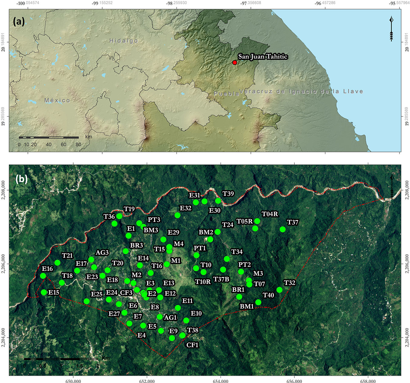
The study was conducted in San Juan Tahitic (19° 56′ 12.7″ N, 97° 32′ 54.6″ W), a 1464-ha area in the municipality of Zacapoaxtla, state of Puebla, Central Mexico (Fig. 1). It is part of the region known as Sierra Norte de Puebla of the Sierra Madre Oriental. Its topographic system corresponds to low and high mountains ranging from 720 to 1800 m a.s.l. in elevation ([20], [22]). It is composed of sedimentary rocks, and regosol is the predominant soil ([20], [22]). The climate is humid-temperate with year-round rainfall ([52]).
Fig. 1 - (a) Location of the study area: San Juan Tahitic (red dot) in the state of Puebla, Central Mexico; (b) the study area (red polygon) and the sampling units (green dots).
The potential vegetation of the area corresponds to cloud forests (CF). This community has very specific environmental requirements, characterized by high annual rainfall, frequent fog, and high atmospheric humidity. This vegetation has a very fragmented distribution, covering only 1.183.800 ha (0.6%) of the Mexican territory ([57], [18]). It is a dense forest made up of several tree strata, where epiphytic and arboreal life forms are of great importance ([47], [12]). Currently, some forests in the study area have been replaced by coffee plantations (CPs) along with rain-fed agriculture ([20]).
Data collection
Sixty-three sampling units (SUs) were established, of which 53 were in areas covered by forests (cloud forests, CF; advanced secondary vegetation, ASV; or shaded coffee plantations, CPs) and the rest (10 SU) in sites with induced vegetation (grasslands and rain-fed agriculture). Each SU consisted of 400 m2 square plots for trees and epiphytes, 100 m2 for shrubs, and 4 m2 for herbs.
For each morphospecies within the SUs, a herbarium specimen was collected ([27]). The variables measured in the field were: (i) density (for trees and shrubs: number of individuals of each species per unit area); (ii) cover (for trees, shrubs, and herbs: proportion of land, occupied by the perpendicular projection of the aerial parts, expressed in m2); (iii) height (trees, shrubs, and herbs); and (iv) diameter at breast height (trees). The epiphytes were only considered for their presence/absence.
Botanical specimens were determined with the help of taxonomic keys or consultation with experts. Data for each species were obtained from public databases ([54]).
Index of Importance for Biological Conservation
Fig. 2 - Flowchart to obtain the index InICoB. Field data collection indicators, raster layers for the geostatistical model..
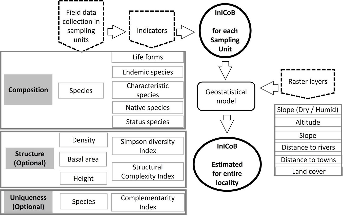
The Index of Importance for Biological Conservation (InICoB, after its Spanish acronym - Fig. 2) is an additive index (eqn. 1) of three weighted variables: composition (C, eqn. 2), structure (E, eqn. 3), and uniqueness (U, eqn. 4). These variables are correlated with the functional aspects of the ecosystem and are integrated by parameters such as the presence and richness of species, diversity or dominance, as well as cover and height of the vegetation, which are excellent indicators of the current, historical conditions and trends of change of the systems ([26], [9], [60], [10], [42]). IniCoB is expressed as follows (eqn. 1):
where Pc (weighting of C) + PE (weighting of E) + PU (weighting of U) = 1; thw weighting depends on plant community (see below). The three components of the index are calculated as follows (eqn. 2 to eqn. 4):
where nij is the number of indicator (i) species in the j-th sampling unit (SU), Nj is the total number of species in the j-th SU, jmax is the maximum value of the ratio nij / Nj observed in the j-th SU. The Simpson’s diversity index (ID - [51]) for the j-th SU is calculated as (eqn. 5):
where n is the number of individuals of a species and N the total number of individuals of all species. The structural complexity index (IC - [19]) at the j-th SU can be estimated as (eqn. 6):
where s is the number of species detected in the j-th SU, d is the density of individuals per unit of area, b is the basal area in the same unit area, and h is the average height. Finally, the average complementarity index (ICom), which reflects the dissimilarity in the species composition of each SU with respect to the rest ([6]) is calculated as (eqn. 7):
where a is the number of species in site A, b the number of species in site B, and c the number of shared species between sites A and B.
Among the advantages of InICoB, there is the easy interpretation of results, because it ranges from 0 (for sites of no importance) to 1 (for sites of high importance for conservation). Additionally, its weighting parameters and composition indicators can be adjusted to any type of plant community and species data (floristic list, optionally forest measurement data).
InICoB applied to cloud forest and associated vegetation
The following weighting was used for the cloud forest (CF) considered in this study: Pc = 0.6, PE =0.3, and PU =0.1. Higher weight was assigned to species composition (C) as several authors ([11], [37], [34]) have reported that after a disturbance, the recovery of species typical of humid forests is slower compared to the recovery of the structure; then, based on the plant list, this variable reflects the degree of conservation of the communities. In contrast, a low weight was given to the uniqueness factor (U, discussed below) because in the study area the secondary/induced plant communities, which are less important for conservation, showed a higher value for this variable.
To quantify the species indicator (ni) in each sampling unit (j), we considered the following: (i) life form (ni1) = number of trees and epiphytes species, which are the best represented life forms of this forest ([46], [47]), and its richness is low in initial or intermediate seral stages; (ii) distribution (ni2) = number of species endemic to Mexico or the Sierra Madre Oriental: this distribution highlights the endemic component; most of the CF species (about 55%) have a neotropical distribution ([46]); (iii) habitat (ni3) = number of species typical of the climax CF; this indicator allows the inclusion of species from other non-dominant life forms that are typical of this ecosystem, such as ferns and lycopods (terrestrial - [46]); (iv) origin (ni4) = number of species native to Mexico; this indicator allows areas covered by secondary or induced vegetation to acquire a non-zero value; (v) status (ni5) = number of species present in the list NOM-059-SEMARNAT-2010 ([50]), the IUCN ([23]) red list and in CITES ([5]); this set adds value when species present a protection or risk status.
The value of InICoB was obtained for each SU, and basic statistics were calculated for the four vegetation communities found in the area: cloud forests (CF), advanced secondary vegetation (ASV) / coffee plantation (CP), agriculture, and induced grasslands. The Kruskal-Wallis and Nemenyi tests ([25]) were performed to compare the InICoB between the communities. Noteworthily, ASV was considered in the same category as shade CPs owing to the difficulty to distinguish them in satellite images ([13]).
Geostatistical model
A beta regression was performed to extrapolate the InICoB to the whole study area in order to predict a continuous dependent variable over the interval (0, 1); it was adjusted under the same distribution (beta) with the use of the mean and precision (phi) parameters. The first parameter (beta) is linked through a link function and a linear predictor, and the second parameter (phi) is linked to a set of regressors through a second link function, resulting in a model with variable dispersion. The estimation was carried out using maximum likelihood procedures, analytical gradients and initial values of an auxiliary linear regression of the transformed response ([61]). The model was developed using the “betareg” library of the R software ([38]), with two types of predictive variables considered: environmental and social (Tab. 1).
Tab. 1 - Predictive variables of the geostatistical model used to extrapolate the InICoB over the whole study area.
| Type | Variable | Character | Categories and abbreviations |
|---|---|---|---|
| Environmental | Altitude | Categorical | Low areas: 720 to 1400 m altitude (A_LOW) High areas: 1400 to 1880 m altitude (A_HIGH) |
| Slope orientation | Categorical | Wet slopes: 0 to 110 and 280 to 360° (S_WET) Dry slopes: 110 to 280° (S_DRY) |
|
| Slope | Quantitative | SLOPE_GR | |
| Distance to rivers | Quantitative | DIST_RIV | |
| Social | Distance to town | Quantitative | DIST_TOWN |
| Distance to roads | Quantitative | DIST_ROAD | |
| Land occupation | Categorical | Cloud forest (V_CF) Advanced secondary vegetation (V_ASV) Initial secondary vegetation (V_ISV) Temporary agriculture (V_AGR) Induced grassland (V_GRA) |
Raster layers were created for each variable using data from the Mexican Continuum of Elevations ([22]), the System for Census Information Consultation ([21]), and the supervised classification of the 2018 SPOT 7 image. The latter layer was obtained using training polygons of known land occupation and the Random Forest algorithm of the R software. All the layers were resampled to a 6-m resolution in order to serve as the basis for further interpolation using the regression model.
Results
Composition and structure indicators
In the 2.52 ha surveyed, 522 vascular plant species were observed; 23 of the sampled sites were covered by different CF associations, 30 by ASV or shade CPs, 7 by grasslands, and 3 by rain-fed agriculture. Tab. 2 and Tab. 3 show the statistics calculated for each composition, structure, and complementarity indicator. All of them present high absolute values in the CF, followed by ASV/CP, and lastly grasslands and agricultural areas, except for the complementarity index (IC), for which the last two associations showed the highest values.
Tab. 2 - Statistics of the composition indicators obtained by each plant community and the entire locality. (CF): cloud forest; (ASV): advanced secondary vegetation; (CP): coffee plantations.
| Group | Community / Stats |
Tree and epiphytic |
Restricted distribution |
Climax species |
Native species |
Conservation status |
Total |
|---|---|---|---|---|---|---|---|
| Average for each plant community |
CF | 20 | 7 | 28 | 32 | 9 | 36 |
| ASV/CP | 17 | 5 | 26 | 32 | 7 | 37 | |
| Grassland | 1 | 2 | 6 | 14 | 1 | 18 | |
| Agriculture | 0 | 2 | 5 | 14 | 1 | 15 | |
| For the whole locality | Mean | 15.56 | 5.33 | 23.54 | 28.94 | 6.75 | 33.3 |
| Standard deviation | 10.15 | 2.88 | 11.89 | 11.15 | 4.77 | 12.8 | |
| Minimum | 0 | 0 | 1 | 7 | 0 | 8 | |
| Maximum | 47 | 12 | 52 | 57 | 19 | 70 |
Tab. 3 - Statistics of the structure and complementarity indexes obtained by plant community and the entire locality. (CF): Cloud Forest; (ASV): Advanced secondary vegetation; (CP): Coffee plantations.
| Group | Community / Stats |
Simpson Index (ID) |
Complexity index (IC) |
Complementarity index (ICom) |
|---|---|---|---|---|
| Average for each plant community |
CF | 0.77 | 28.56 | 0.92 |
| ASV/CP | 0.68 | 11.14 | 0.91 | |
| Grassland | 0.09 | 0.0003 | 0.96 | |
| Agriculture | 0 | 0 | 0.98 | |
| For locality | Mean | 0.6 | 16.0 | 0.92 |
| Standard deviation | 0.3 | 22.9 | 0.03 | |
| Minimum | 0.0 | 0.0 | 0.87 | |
| Maximum | 0.9 | 112.4 | 0.99 |
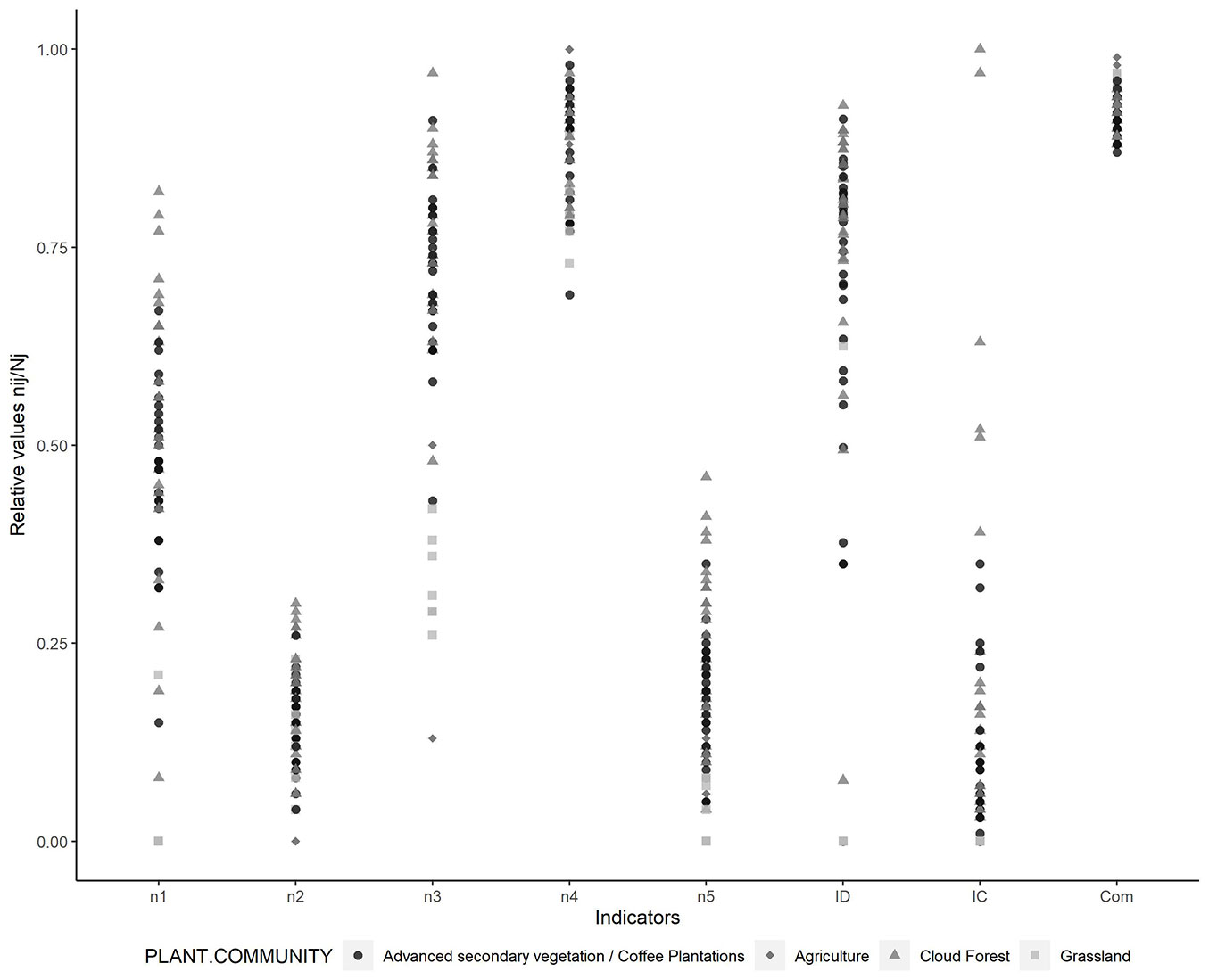
Fig. 3 shows the relative values of the different indicators, where the proportion of native species (n4) in areas covered by agriculture and grasslands have higher values than several sites covered by forest. The indicators referring to the proportion of trees, epiphytes, and climax species, as well as the diversity and structural complexity index show a wide variation, with the CF acquiring the highest values.
Fig. 3 - Relative values of the indicators that make up the InICoB for the different plant communities.
InICoB applied to the cloud forest
The average InICoB for the entire locality was 0.61, with the maximum recorded value of 0.91 and the minimum value of 0.30. Fig. 4 shows the lowest InICoB values in areas with agriculture and grasslands. The CF presents the highest InICoB average, although its variability overlaps with the values recorded for sites covered with ASV/CP.
Fig. 4 - Variation in InICoB in the different plant communities and significant differences between them.
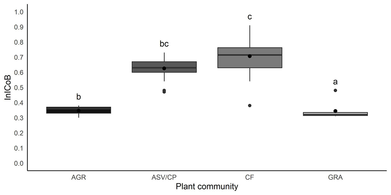
According to the Kruskal-Wallis test, significant differences (p<0.001) were found in the InICoB average values calculated for the different plant communities. CF associations were significantly different from the rest of the communities after Nemenyi test, while agricultural areas did not show significant differences with the ASV/CAF and the grasslands (Fig. 4).
Geostatistical model
Two geostatistical models were adjusted to extrapolate the InICoB to the entire study area. Model 1 included all the variables (environmental and social) proposed in the method, and model 2 considered only the six significant variables. For categorical variables, the most frequent categories were represented in the intercept; these were as follows: slopes with humid orientation (S_WET), high altitude zones (A_HIGH), and CF coverage (V_CF). In this model, distance to town (DIST_TOWN), advanced secondary vegetation (V_ASV), agriculture (V_AGR), and induced grassland coverage (V_GRA) were significant (p < 0.05).
Although models 1 and 2 presented good adjustment (pseudo R2 = 0.69 and 0.70, respectively) and an error of 7%, model 2 had the lowest value of the Akaike information criterion. This indicates that model 2 has a better adjustment along with less complexity; therefore, it has higher quality to predict and perform the interpolation (Tab. 4).
Tab. 4 - Geostatistical model and adjustment parameters. (O_SEC): dry slopes; (A_BAJ): low altitudes; (PEND_GR): slope; (DIST_RIOS): distance to rivers; (DIST_POB): distance to towns; (V_VSA): Advanced Secondary Vegetation; (V_VSI): Initial Secondary Vegetation; (V_AGR): Agriculture; (V_PAS): Induced grassland; (RMSE): Root mean square error. (*): significant variables.
| Variable | Model 1 | Model 2 | ||
|---|---|---|---|---|
| Parameter | Prob. | Parameter | Prob. | |
| Intercept | 3.978-01 | 0.121 | 0.487 | 0.0003 |
| S_DRY | 2.498-02 | 0.835 | - | - |
| A_LOW | 2.872-02 | 0.862 | - | - |
| SLOPE_GR | 1.136-02 | 0.055 | 0.011 | 0.0506 |
| DIST_RIV | 1.251-04 | 0.359 | - | - |
| DIST_TOWN* | 2.451-04 | 0.002 | 0.0003 | 1.72-05 |
| V_ASV* | -1.771-01 | 0.00061 | -0.167 | 0.0011 |
| V_ISV | -2.103-01 | 0.088 | -0.184 | 0.114 |
| V_AGR* | -3.050-01 | 4.77-08 | -0.308 | 2.67-08 |
| V_GRA* | -2.919-01 | <2-16 | -0.285 | <2-16 |
| Pseudo R2 | 0.7087 | 0.6978 | ||
| RMSE | 0.0732 | 0.0737 | ||
| AIC | -125.104 | -129.331 | ||
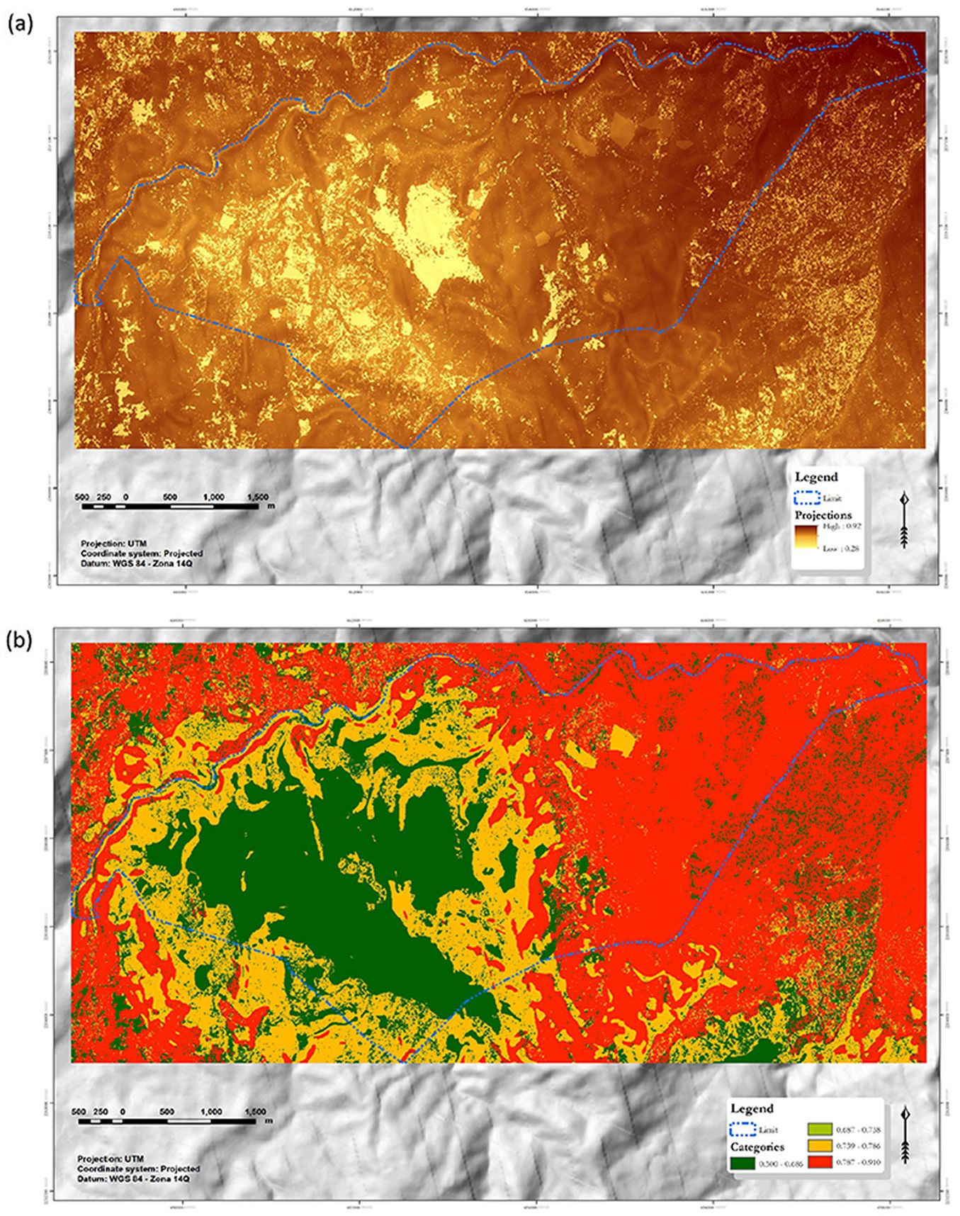
The extrapolation based on model 2 shows that the eastern part of the study area has the highest InICoB values, while the lowest values are concentrated in the center and scattered to the west of the locality. To simplify the visualization, the InICoB was reclassified into four categories based on the quantiles; therefore, each category represents 25% of the surface (Fig. 5).
Fig. 5 - InICoB applied to the San Juan Tahitic locality. (a) InICoB in continuous values, and (b) InICoB divided into four quantiles.
Discussion
Composition and structure indicators’ relevance
The composition and structure indicators (list of species and forest measurement data) used to calculate the InICoB are basic information for environmental characterization and diagnosis. Some of these variables have already been used ([16], [30], [42], [53], [32]). According to our results, the indicators proposed for the InICoB allow the identification of areas of importance for the conservation of natural biodiversity and the monitoring of their status.
Almost all the SUs corresponding to the CF obtained the highest scores for all the indicators, except the associations dominated by Pinus spp. or Platanus mexicana; although these are climax associations, they are less rich in tree species, and therefore offer less variety of habitat for epiphytes and herbaceous plants. In addition, the dominance of a few species generates lower diversity values. Both characteristics result in a lower total InICoB value.
The SUs covered by CPs obtained medium to high values; some SUs of other classes even surpassed the sites with the less diverse associations of the CF ([31], [3]). Evidently, this agroforestry system is a refuge for a high number of CF species. Most of the sites with ASV presented medium to low values. This can be explained by several factors: in the study area, this successional stage is usually dominated by Alnus acuminata or Liquidambar styraciflua, and such dominance generates low diversity values. Additionally, young forests have a low structural complexity; their height and basal area are lower in comparison with mature forests, and the dominant species are characterized by being poor phorophytes, reducing the richness of epiphytes.
As expected, the SUs occupied by agricultural activities and induced grasslands showed the lowest values for most of the indicators, except for the complementarity index. This parameter evaluates the proportion of species that are unique in an association. The complementarity value indicates that the induced vegetation with unique species contributes to the overall biodiversity of the region, since some of its species are not present in the forest communities.
Validation of the index
We consider that the InICoB applied to temperate forests should assign a higher weight to composition (PC = 0.6), a medium value to structure (PE = 0.3), and a low value to uniqueness (PU = 0.1). The higher weight assigned to composition is supported by the fact that particularly in this kind of forest, species composition is more sensitive to disturbance and its recovery is slower and more difficult ([35], [11], [37], [34]). Although the uniqueness factor qualifies the contribution that each association makes to the total diversity of the region, the associations that presented the greatest differences in the composition of species and that obtained the highest values of uniqueness are those formed by induced vegetation (agricultural and grassland); therefore, a low weight was assigned to this factor.
InICoB adequately evaluates the biological importance of the vegetation in the study area. Some areas covered by ASV/CP showed InICoB values equal to or higher than some CF sites; these areas have considerable biological importance for conservation because they are comprised of numerous climax species of the CF ([31], [3]) that add importance to these sites.
InICoB extrapolation
When evaluating the effect of environmental and social variables on InICoB, land occupation has the greatest influence. Induced plant communities such as agricultural zones and grasslands have a more negative effect on InICoB than secondary vegetation. Distance to town is another social variable that affects this index; however, it has a positive correlation with IniCoB: the farther the distance from the rural center, the higher the index.
Slope has a small and positive correlation with InICoB. Although it is strictly an environmental variable, it can also be indirectly influenced by non-natural impacts; in steeper slopes, the land use change is more difficult. These observations coincide with Williams-Linera et al. ([59]) in a CF in Veracruz, Mexico.
Other environmental variables such as altitude and slope orientation (which directly influence relative humidity) have no significant correlation with InICoB in the study area. The effect of these variables is probably limited by the high humidity of the region. However, in subhumid to dry communities, as well as in larger areas or those with a higher environmental heterogeneity, these factors could have an influence on the richness and composition of plant species, as recorded by Gallardo-Cruz ([15]), Cielo-Filho et al. ([4]), and Luis-Martínez et al. ([28]) for seasonal tropical forests, and by Wang et al. ([58]), Zhao et al. ([62]), Romero et al. ([44]), and Ramírez-Prieto et al. ([40]) for subhumid to dry temperate forest communities.
InICoB Application
InICoB is a flexible index, according to the field data, as it can be applied to any type of vegetation and adjusted to different objectives or types of samplings.
For diverse types of vegetation, the indicators of life form and species distribution could be adjusted. The expected life form spectrum of each plant community must be considered. For example, perennial herbs (hemicryptophyte type) are the representative form in cold forests; shrubs and subshrubs with annual herbs predominate in dry temperate climates; perennial herbs (geophytes) in Mediterranean climates and trees in warm systems ([47], [29] [39]).
The indicator corresponding to the distribution of species has the objective of adding importance when the site has endemic plants; therefore, this parameter depends on the location of the study area. For example, the arid zones of northern Mexico and the southern USA have a high quantity of locally endemic elements; however, in the southern tropical zones, where many species reach Central and South America, Mexican elements can be good indicators ([45]).
Regarding sampling and the type of information collected, many floristic studies lack forest measurement data, either because of the scope of their objectives or because of the costs involved. In these cases, InICoB could be calculated by setting a value of zero for structure (PE), using only the composition and uniqueness variables.
The uniqueness factor is relevant when there are important, unique communities that need to be considered for conservation, for example aquatic associations, in which case a higher value could be assigned to this factor.
InICoB relies on species composition and structure, and its indicators are quantitative, based on the number of species or on already established (quantitative) indices. The only subjectivity is in the attribution of weights to the factors (composition, structure, and uniqueness), and this confers flexibility according to the data collected or the project’s objectives.
Another advantage is that InICoB is mainly based on the floristic list; this is the base data for environmental diagnosis and, therefore, does not require specialized information. It is easy to interpret because its values range from 0 to 1, and it can be visualized on a spatial scale; therefore, a raster layer can be generated to add other data.
However, to prove the effectiveness of IniCoB, it should be tested with changes in the weighting of the factors, or changes in the species indicators to evaluate other plant communities.
Conclusions
The InICoB indicators, based on composition and structural variables of the vegetation, are relatively easy to obtain. They are based on a list of species as well as forest measurement data. Additionally, they are quantitative and, therefore, lack subjectivity. The proposed index facilitated the spatial evaluation of the importance of biological conservation in the studied area and its changes in space. The values obtained are easy to interpret and easily comparable across studies. InICoB also distinguishes different plant communities, assigning higher values to the CF than to the rest of the secondary or induced plant communities. Further, this index can be flexible and adjusted to the available data. However, its quality with respect to its application to other plant communities should be tested.
List of abbreviation
The following abbreviations have been used throughout the text:
- Advanced Secondary Vegetation (ASV);
- Cloud Forest (CF);
- Coffee Plantations (CP);
- Index of Importance for the Biological Conservation (InICoB);
- Sample units (SU).
Acknowledgments
ANTD conceived the study, did the conceptualization, methods, carried out the field data collection, curation and analysis, writing, review, and editing; MJGG helped with the conceptualization, review, and carried out the supervision and project administration; HMSP helped with the conceptualization and formal analysis; PHR helped with the conceptualization, methodology, and writing; ALM helped with the review and editing.
We thank Dr. Jonathan Amith for commenting on the manuscript in the English version. We also thank Canek Ledesma Corral, Anastasio Sotero Hernández, Misael Andrés García, Lucía Freiré, and Erika Servín for their collaboration in collecting the field data.
This study was partially supported by CONAHCYT scholarship, program no. 000103, and by the Colegio de Postgraduados, Texcoco, Mexico.
References
CrossRef | Gscholar
Gscholar
Gscholar
Online | Gscholar
Gscholar
Gscholar
Gscholar
Gscholar
Gscholar
Gscholar
CrossRef | Gscholar
Gscholar
Gscholar
Gscholar
Gscholar
CrossRef | Gscholar
Online | Gscholar
Gscholar
CrossRef | Gscholar
Authors’ Info
Authors’ Affiliation
Manuel de Jesús González-Guillén 0000-0003-1814-4320
Héctor Manuel De Los Santos Posadas 0000-0003-4076-5043
Patricia Hernández De La Rosa 0000-0001-8577-1127
Aurelio León Merino 0000-0002-0885-5084
Colegio de Postgraduados, km. 36.5 Carr. Mexico-Texcoco, Montecillo, Texcoco, C.P. 56230 (Mexico)
Corresponding author
Paper Info
Citation
Torres-Díaz AN, González-Guillén MJ, De Los Santos Posadas HM, Hernández De La Rosa P, León Merino A (2023). A new zoning index for detecting areas of biological importance applied to a temperate forest in Central Mexico. iForest 16: 253-261. - doi: 10.3832/ifor4111-016
Academic Editor
Marco Borghetti
Paper history
Received: Apr 08, 2022
Accepted: Jul 04, 2023
First online: Aug 31, 2023
Publication Date: Aug 31, 2023
Publication Time: 1.93 months
Copyright Information
© SISEF - The Italian Society of Silviculture and Forest Ecology 2023
Open Access
This article is distributed under the terms of the Creative Commons Attribution-Non Commercial 4.0 International (https://creativecommons.org/licenses/by-nc/4.0/), which permits unrestricted use, distribution, and reproduction in any medium, provided you give appropriate credit to the original author(s) and the source, provide a link to the Creative Commons license, and indicate if changes were made.

Web Metrics
Breakdown by View Type
Article Usage
Total Article Views: 20600
(from publication date up to now)
Breakdown by View Type
HTML Page Views: 15625
Abstract Page Views: 2649
PDF Downloads: 1888
Citation/Reference Downloads: 4
XML Downloads: 434
Web Metrics
Days since publication: 1028
Overall contacts: 20600
Avg. contacts per week: 140.27
Article Citations
Article citations are based on data periodically collected from the Clarivate Web of Science web site
(last update: Mar 2025)
(No citations were found up to date. Please come back later)
Publication Metrics
by Dimensions ©
Articles citing this article
List of the papers citing this article based on CrossRef Cited-by.
Related Contents
iForest Similar Articles
Research Articles
Bird response to forest structure and composition and implications for sustainable mountain forest management
vol. 19, pp. 18-27 (online: 11 January 2026)
Research Articles
Exploring patterns, drivers and structure of plant community composition in alien Robinia pseudoacacia secondary woodlands
vol. 11, pp. 586-593 (online: 25 September 2018)
Research Articles
Enhancing forest biodiversity indicators in inventories through harmonized protocols
vol. 18, pp. 109-120 (online: 20 May 2025)
Research Articles
Diversity of saproxylic beetle communities in chestnut agroforestry systems
vol. 13, pp. 456-465 (online: 07 October 2020)
Research Articles
Effects of different silvicultural measures on plant diversity - the case of the Illyrian Fagus sylvatica habitat type (Natura 2000)
vol. 9, pp. 318-324 (online: 22 October 2015)
Technical Reports
Assessment of allergenic potential in urban forests: a case study of the Royal Park of Portici in Southern Italy
vol. 13, pp. 376-381 (online: 25 August 2020)
Research Articles
Influence of pH, nitrogen and sulphur deposition on species composition of lowland and montane coniferous communities in the Tatrzanski and Slowinski National Parks, Poland
vol. 12, pp. 141-148 (online: 27 February 2019)
Research Articles
Distribution of juveniles of tree species along a canopy closure gradient in a tropical cloud forest of the Venezuelan Andes
vol. 9, pp. 363-369 (online: 08 December 2015)
Short Communications
Towards cost-effective indicators to maintain Natura 2000 sites in favourable conservation status. Preliminary results from Cansiglio and New Forest
vol. 1, pp. 75-80 (online: 28 February 2008)
Research Articles
Clonal structure and dynamics of peripheral Populus tremula L. populations
vol. 7, pp. 140-149 (online: 13 January 2014)
iForest Database Search
Google Scholar Search
Citing Articles
Search By Author
Search By Keywords


