Enhancing forest biodiversity indicators in inventories through harmonized protocols
iForest - Biogeosciences and Forestry, Volume 18, Issue 3, Pages 109-120 (2025)
doi: https://doi.org/10.3832/ifor4778-018
Published: May 20, 2025 - Copyright © 2025 SISEF
Research Articles
Abstract
Forest biodiversity is a multifaceted term encompassing tree and shrub diversity and the diversity of other life forms such as animals or fungi. Extensive forest monitoring networks such as National Forest Inventories or the International Co-operative Programme on Assessment and Monitoring of Air Pollution Effects on Forest plots have implemented biodiversity-monitoring protocols to satisfy increasing information demands. However, these protocols often evaluate biodiversity through potential biodiversity indicators (e.g., stand structure and deadwood), which may not provide sufficient information on other aspects of the current forest biodiversity status. In this study, we present the forest biodiversity monitoring results and lessons from a cross-country study to support large-scale monitoring systems. We developed, evaluated, and discussed harmonized protocols, mainly focused on birds and mammals, which extend beyond the traditional features captured in large-scale forest inventories. We leverage information from 30 intensively monitored plots established in six European countries to achieve these goals. The protocols were helpful in recording data that could be used to reproduce biodiversity-related attributes such as measures of forest structure, regeneration, deadwood features, and bird and mammal diversity. Specifically, field data on trees was used to describe structural features of forests such as stand composition and forest complexity. In contrast, composition and regeneration data provided helpful information for other biodiversity indicators. Data gathering to monitor bird and mammal diversity requires revisiting the plots, which involves greater economic investment and human effort. Once the bird and mammal data have been collected, advanced algorithms could facilitate and enhance the efficiency of the analyses. To optimize the monitoring efficiency, we recommend including these two new biodiversity assessments in a subset of extensive survey plots. Furthermore, using standard guidelines for these new assessments across all countries would facilitate the comparison and reporting of statistical data.
Keywords
Avian Diversity, Ecology, Harmonization, Management, Reporting, Sustainability
Introduction
According to the State of the World’s Forests, forests cover 31 per cent of the earth’s land area and contain 80 per cent of the world’s terrestrial plant and animal species ([19]). Forests also provide numerous ecosystem services, including the provisioning of raw materials and the regulation of geochemical cycles ([9]). Forest biodiversity is a complex term embracing various concepts, with the number of species in a given area (i.e., species richness) often being the most relevant ([71]), although this can be a biased indicator ([41]). This conceptualization has been extended to include other levels of organization, such as gene or ecosystem components ([35]). Additionally, there is an increasing awareness of functional diversity, i.e., focusing on the kind of species (using single- or multi-level traits) rather than their numbers and forest structural complexity ([41]).
In recent years, the need to enhance knowledge regarding the State of Europe’s forests ([22]), their trends, and their resilience has become increasingly critical, as highlighted in the new European Forest Strategy for 2030 and the Proposal for a Regulation on a monitoring framework for resilient European forests. Addressing this challenge requires developing a comprehensive and harmonized set of biodiversity indicators. Given the inherent complexity of biodiversity assessment, a significant portion of these indicators must be derived from field data. Consequently, efforts to standardize field protocols, harmonize indicator methodologies, and incorporate new biodiversity variables into large-scale monitoring frameworks represent a valuable opportunity to advance our understanding of forest ecosystems ([76]).
Assessing plant-species diversity is common in some forest inventories ([47]). However, quantifying species diversity in forest inventories has mainly focused on trees and, to a lesser extent, shrubs and bush species. In contrast, grasses, herbs, and other non-woody species have received less attention ([14]). Beyond estimating species richness, identifying the species present in each area allows to consider relevant species, such as endangered or red-listed, non-native species, or umbrella species ([29]). Regarding umbrella species, we refer to the Lambeck ([40]) definition, i.e., “those whose requirements are believed to encapsulate the needs of other species”. A discussion on the suitability of umbrella species as surrogates of diversity can be found in Wang et al. ([78]).
The quantification of species diversity in forest ecosystems should not be restricted to plant species (trees, shrubs, herbs, ferns) but it should also encompass other organisms like animals (both vertebrate and invertebrate), lichens, bryophytes, and microorganisms, such as bacteria, viruses, and fungi ([8], [9], [72]). A comprehensive evaluation of such a large array of life forms is complex and would require extensive sampling efforts ([72]). To simplify this task, extensive forest inventories develop proxies of forest biodiversity. Several proxies allow to estimate potential biodiversity, such as umbrella species, surrogate species, or biodiversity indicators ([32]).
We consider indicators as a metric that represents the state of a variable or system ([37]). In this regard, the State of Europe’s Forests ([22]) includes 10 biological diversity indicators for forest ecosystems: (i) diversity of tree species; (ii) regeneration; (iii) naturalness; (iv) introduced tree species; (v) deadwood; (vi) genetic resources; (vii) forest fragmentation; (viii) threatened forest species; (ix) protected forests; (x) common bird species.
Diversity of tree species as well as regeneration can easily be derived from extensive inventories such as National Forest Inventories (NFIs) or the International Co-operative Programme on Assessment and Monitoring of Air Pollution Effects on Forest (ICP) plots ([16], [47]). Similarly, the suitability of these networks for monitoring the status and dynamics of invasive species has been proven ([33]), while using these probabilistic designs for detecting rare species may be limited ([12]).
Deadwood is a habitat for organisms such as bryophytes, arthropods, fungi, lichens, and other life forms ([55], [54]). Deadwood surveys consist of sampling both standing and lying deadwood pieces and are widespread in research plots and extensive monitoring networks ([65]). These surveys are based on different sampling strategies with linear intersect transects (e.g., Switzerland) and fixed area plots (e.g., Spain) being the most common ([79]). However, deadwood stocks cannot be the sole indicator of biodiversity and must be complemented by other attributes such as the deadwood type or deadwood decay class ([54]).
Forest structure, i.e., the size and spatial distribution of trees within the stand, species composition, and tree size diversity ([58]) can be evaluated via spatially or non-spatially explicit indices ([46]) derived from forest inventories used for research purposes ([7]), as well as management plans ([80]) and NFIs ([46], [49]). In addition, remote sensing techniques, such as laser scanning, have gained increasing importance for evaluating forest structure ([36]). Complex forest structures, i.e., stands with large differences in tree diameters, all-age and multispecies forests, are associated with higher levels of biodiversity ([20], [55]). Furthermore, certain organisms such as birds, insects, bryophytes, or lichens inhabit old and damaged trees ([44], [24]).
Some of the forest attributes described here, such as naturalness, deadwood stocks, structure, and old-growth stands, are assumed to be linked to animal diversity ([55]). However, in some circumstances, the association between animal species and the place they inhabit is poorly documented ([41]). Therefore, it seems appropriate to undertake more exhaustive surveys in this regard. In the case of birds and bats, the range of survey alternatives is extensive, ranging from birdwatching to song/vocalization recognition, as well as combined approaches ([31]). Identification from song can be achieved using traditional field methods such as the point-count method, linear transects, or bioacoustic recorders ([63], [69]). Regarding other groups of animals, there is also a wide range of survey alternatives, such as track identification, direct observation, faeces identification, trapping, and phototrapping using cameras ([28], [52]).
Biodiversity field protocols have expanded towards other levels, such as the gene level (see, for example, the initiatives led by the European Forest Genetic Resource Programme - [18]). The quantification of genetic diversity is highly valuable given the relationship to tree survival and adaptive processes under changing environmental conditions, as well as ensuring that forest vitality is such that they can cope with pests and diseases ([39]). A primary limitation in assessing genetic diversity is the high cost of collecting plant material and the subsequent expensive analyses ([53]). Another aspect which is increasingly gaining importance is the evaluation of soil communities, given the close link with ecosystem functionality, and the fact that they host a large number of life forms which can interact with plants ([48], [68]). Metabarcoding is a widely used technique for assessing soil biodiversity, requiring the collection of soil samples, storage under standardized conditions, subsequent DNA extraction, and amplifying the genes of interest ([11], [45]).
NFIs and ICP forest plots are one of the main sources of information on forest resources at national and international levels and are used to report forest indicators to international organizations ([76]). In addition to reporting data on forest attributes (e.g., stocks, growth, or regeneration), they can provide data on biodiversity indicators such as deadwood stocks, forest structure, ground vegetation, or stand composition ([14]). However, these indicators can only assess potential biodiversity. Still, to obtain robust forest information comparable among countries, these indicators need to be harmonized, i.e., using the same reference definitions and methodology ([4]). In this regard, biodiversity estimation and cross-country comparability have proven to be very complicated in long-term forest inventories ([14]) since the origins of these inventories and the field biodiversity protocols differ. For example, the Spanish NFI in its Third cycle recorded lichen diversity data and later discarded it because of the taxonomic complexity, the need for field experts, and the low efficiency involved (monitoring costs and time spent). Similarly, the Swiss NFI started collecting information on ants and subsequently decided against it. Therefore, a harmonisation process, particularly considering the same reference definitions, is key to ensuring comparability among the data from different countries ([76]). In this regard, cross-country pilot initiatives play an important role in terms of proposing new technologies and analysing their operability and ease of use for estimating biodiversity indicators and, in turn, identifying the best options to obtain robust, large-scale information for decision-making and promoting sustainable forest management across Europe.
In this study, we developed, evaluated, and tested standardised protocols for large-scale monitoring of current biodiversity. We considered both the components that are already monitored through large-scale inventories but need to be further harmonised and those beyond the traditional attributes that are currently captured in forest inventories. These protocols were applied in a pilot study encompassing 30 intensively monitored plots in six countries covering a broad spectrum of European forest types ([6]). The core biodiversity monitoring aspects considered in the harmonised protocols include: (i) forest structure; (ii) regeneration; (iii) deadwood; (iv) bird diversity; and (v) mammal diversity.
Materials and methods
Plot descriptions
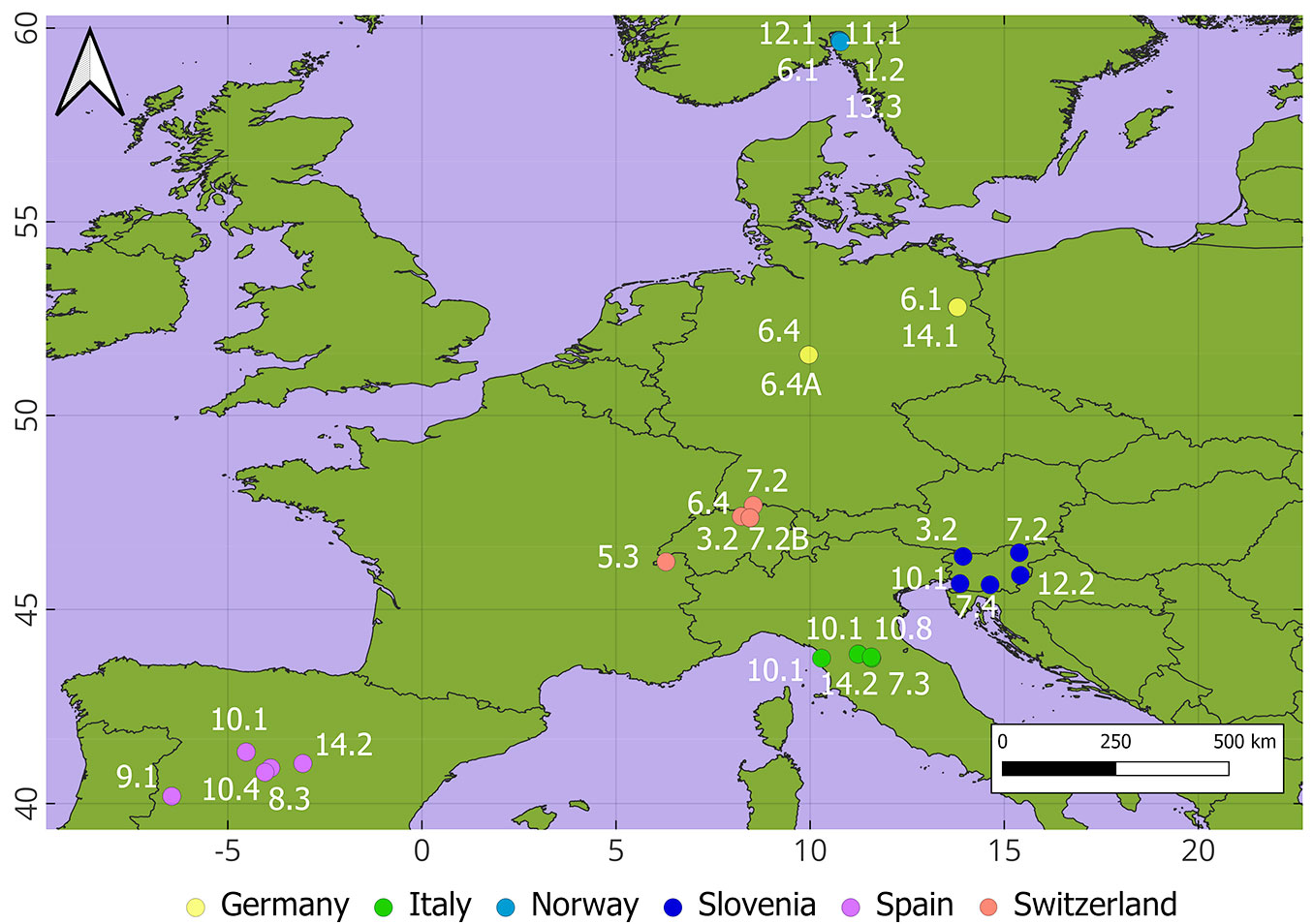
Within the framework of the Pathfinder HE project ([56]), six countries agreed on establishing five plots (N total = 30 plots) in different forest types with the objectives of comparing dendrometric data obtained using classical measures with terrestrial LiDAR and evaluating harmonized measurements for biodiversity evaluation (Tab. 1, Fig. 1). Project partners were encouraged to establish plots in representative forest types within each country to capture the widest possible range of forest types across Europe. The plots encompassed 13 out of the 14 categories of the European Forest Types ([6]). The plots established were square-shaped with a size of 2500 m2 (50 × 50 m). All the trees with a diameter at breast height (dbh) larger than 7 cm were identified, mapped with a submetric GNSS and their dbh and height were measured. Note that “forest type” refers here to a specific plot rather than the entire forest type.
Tab. 1 - Main forest attributes of the sampled plots. Coordinates are in km according to ERTS89-extended LAEA (3035); Mean DBH is the plot mean diameter in cm; BA is the basal area in m2 ha-1; and N is the number of trees per ha.
| Country | EU Forest type | Coordinates | Mean DBH |
Basal area |
N |
|---|---|---|---|---|---|
| Spain | 9.1 Mediterranean evergreen oak forest | 2926; 2051 | 39.2 | 22.9 | 184 |
| 10.1 Thermophilous pine forest | 3108; 2142 | 17.8 | 14.1 | 316 | |
| 8.3 Pyrenean oak forest | 3153; 2087 | 19.2 | 24.6 | 804 | |
| 10.4 Mediterranean and Anatolian Scots pine forest | 3138; 2078 | 30.6 | 49.2 | 636 | |
| 14.2 Plantations of non-site-native species and self-sown exotic forest | 3224; 2088 | 26.8 | 30.5 | 516 | |
| Germany | 6.1. Lowland beech forest of southern Scandinavia and north central Europe spruce-silver fir forest | 4576; 3306 | 29.7 | 28.1 | 284 |
| 14.1 Plantations of site-native species | 4577; 3306 | 24.6 | 30.3 | 616 | |
| 6.4A Central European submountainous beech forest | 4318; 3162 | 20.5 | 19.6 | 308 | |
| 6.4 Central European submountainous beech forest | 4318; 3162 | 27.4 | 23.8 | 280 | |
| Norway | 6.1 Lowland beech forest of southern Scandinavia and north central Europe. | 4363; 4066 | 23.7 | 42.7 | 668 |
| 12.1 Riparian forest | 4364; 4065 | 17.4 | 44.4 | 1860 | |
| 2.1 Hemiboreal forest | 4364; 4064 | 20.8 | 31.0 | 652 | |
| 11.1 Spruce mire forest | 4365; 4064 | 14.4 | 21.3 | 1100 | |
| 13.3 Mountain birch forest | 4365; 4061 | 15.7 | 21.3 | 1124 | |
| 1.2 Pine-dominated boreal forest | 4365; 4061 | 25.7 | 27.7 | 532 | |
| Switzerland | 5.3 Ashwood and oak -ash forest | 4034; 2576 | 23.4 | 39.5 | 616 |
| 7.2 Central European mountainous beech forest | 4211; 2731 | 58.2 | 33.2 | 116 | |
| 6.4 Central European submountainous beech forest | 4187; 2700 | 44.2 | 35.5 | 176 | |
| 7.2.B Central European mountainous beech forest | 4204; 2696 | 31.9 | 25.5 | 276 | |
| 3.2. Subalpine and mountainous spruce and mountainous mixed spruce-silver fir forest | 4204; 2696 | 19.9 | 38.6 | 732 | |
| Slovenia | 3.2 Subalpine and mountainous spruce and mountainous mixed spruce-silver fir forest | 4624; 2592 | 53.6 | 70.7 | 308 |
| 12.2 Fluvial forest | 4742; 2545 | 38.9 | 33.7 | 228 | |
| 7.2 Central European mountainous beech forest | 4735; 2609 | 38.0 | 47.4 | 372 | |
| 10.1 Thermophilous pine forest | 4622; 2514 | 21.8 | 34.0 | 664 | |
| 7.4 llyrian mountainous beech forest | 4683; 2514 | 27.8 | 33.4 | 412 | |
| Italy | 14.2 Plantations of non-site-native species and self-sown exotic forest | 4448; 2298 | 46.4 | 61.2 | 328 |
| 10.8 Cypress forest | 4421; 2306 | 25.0 | 38.9 | 700 | |
| 7.3 Apennine-Corsican mountainous beech forest | 4449; 2294 | 31.4 | 34.7 | 400 | |
| 10.1 Thermophilous pine forest | 4421; 2305 | 16.7 | 21.8 | 852 | |
| 10.1B Thermophilous pine forest | 4345; 2293 | 67.1 | 18.6 | 52 |
Fig. 1 - Location of the plots. Codes refer to the European Forest Types as defined by Barbati et al. ([6]) (Table 1). Colors refer to the six countries.
We reviewed some of the most commonly used indices for forest structure quantification and, to attain a deeper understanding of biodiversity, presented harmonised protocols for the estimation of deadwood, regeneration, and richness of vertebrate animals (birds and mammals).
Forest structural indices
In this study, five indices were considered to characterize the forest complexity and species mingling: (i) forest complexity using the sum of Square Roots of differences Index (SQRI, eqn. 1 - [7]); (ii) spatial pattern of the trees using the Clark and Evans Aggregation Index (CE, eqn. 2 - [15]); (iii) the size differentiation (DIFF, eqn. 3), i.e., spatial size inequality in trees using the Gadow’s Index ([77]); (iv) species mingling using the index MINGL (eqn. 4) proposed by Aguirre et al. ([2]); and (v) species diversity through Shannon’s Diversity Index (SI, eqn. 5 - [70]).
High values of SQRI are related to more complex stands (eqn. 1):
where i refers to the i-th tree, n to the total number of trees, and pi is the relative proportion of the total basal area of each tree, dbh is the diameter at breast height of the tree i and DBH is the mean plot diameter.
The CE index compares the observed mean nearest neighbour distance (r) in the pattern to that expected for a Poisson point process of the same intensity (eqn. 2):
A value of CE < 1 suggests aggregation or clustering, CE > 1 suggests a regular spatial pattern, while CE = 1 indicates a random spatial pattern.
The DIFF index aggregates the smaller and larger dbh ratios of the k (k = 3) nearest neighbours (eqn. 3):
DIFF = 0 implies that neighbouring trees share similar dbh, while large index values are associated with increasing dbh differences between neighbouring trees.
MINGL quantifies the spatial pattern of the species (eqn. 4):
Low MINGL index values suggest intermingling or species attraction, whereas high values indicate species repulsion.
The SI index quantifies the species diversity (eqn. 5):
where g is the relative basal area of the l-th species (S = 2, …, S). High values of this index suggest more diverse forests in terms of species composition.
CE, DIFF, and MINGL are spatially explicit and, therefore, require an edge effect in the trees close to the plot boundaries. For the DIFF and MINGL, we applied the NN1 edge correction method ([59]) and the cumulative distribution function method for the CE.
We also performed Non-Metric Multidimensional Scaling (NMDS) and a Bray-Curtis community dissimilarity distance matrix to represent the structural variability among forest types. We also calculated the stress value as a measure of goodness of fit. As a rule of thumb, values lower than 0.2 are assumed to suggest a good representation of the data. Finally, we represented the forest types in a two-dimensional reduced space. TD and SM were calculated using the “treespat” ([61]), CE using the “spatstat” packages ([5]), and NMDS was run using the “vegan” package ([51]) implemented in R ver. 4.3.3.
Forest regeneration
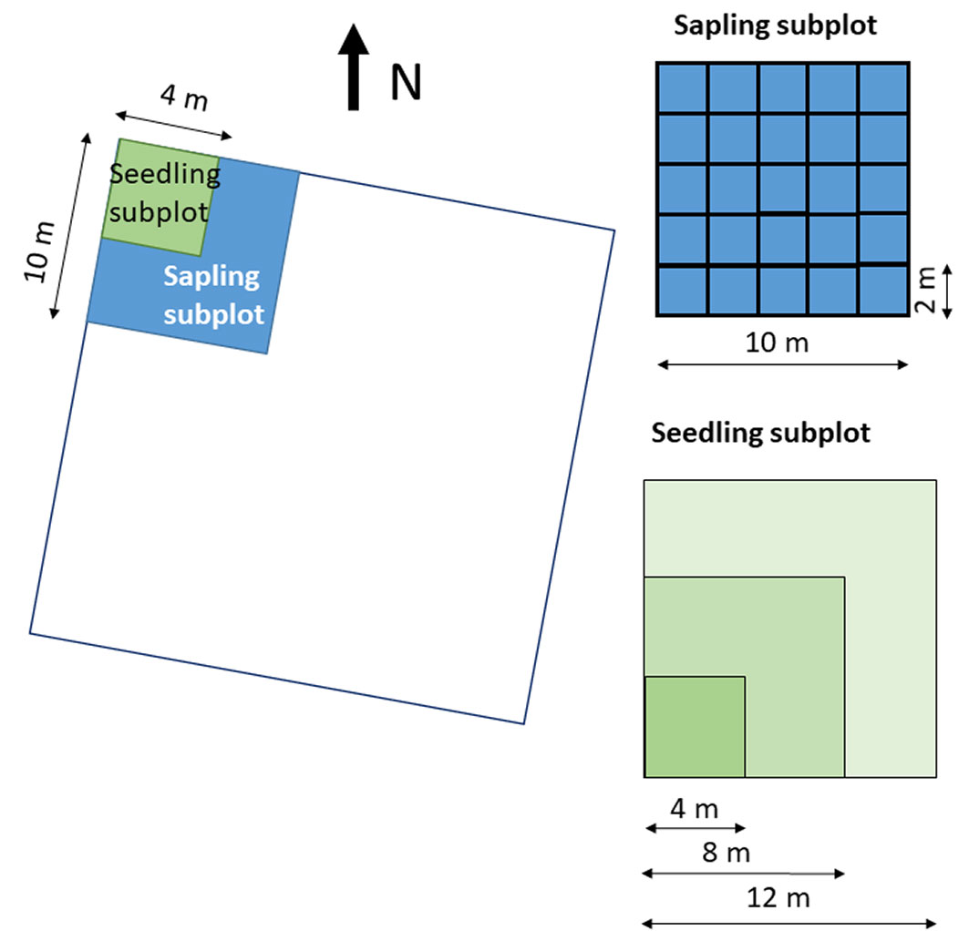
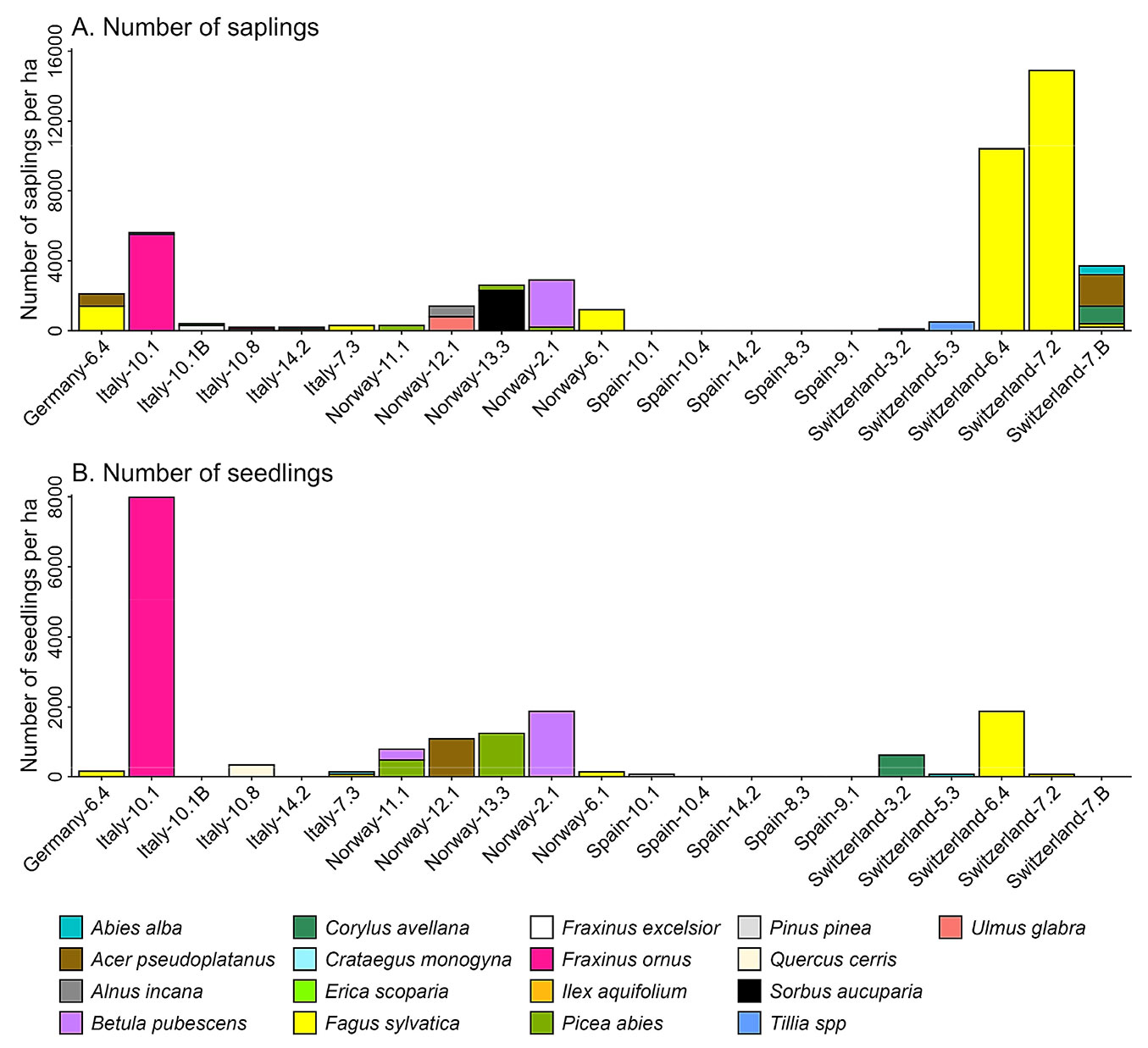
We specified two categories of regeneration: seedlings and saplings. Seedlings (individuals with height ≥ 50 cm and dbh < 2 cm) were counted within a subplot of 4 × 4 m located in the northernmost corner of the plot. In cases where seedlings were not present in the subplot, the survey area had to be expanded to a square of 8 × 8 m and up to 12 × 12 m. The saplings (recruits with 2 cm ≤ dbh < 7 cm) were counted within a grid of 10 × 10 m split into 25 cells of 2 × 2 m (Fig. 2). This grid was also established in the northernmost corner of the plot.
Fig. 2 - Schematic representation of the seedling and sapling subplots.
Regeneration data (i.e., seedling and sapling data) were collected in 23 plots: one in Germany, five in Italy, six in Norway, five in Spain and five in Switzerland. The indicator considered was the number of seedlings and saplings by forest type.
Deadwood
Deadwood data was collected in the whole plot, classified into the following three typologies and recorded diameter: (i) dead standing trees (dbh ≥ 7.0 cm, height ≥ 1.3 m); (ii) dead-lying trees and branches (diameter at 1 m from the base ≥7.0 cm and length ≥1 m); (iii) stumps/snags (diameter at mid-height ≥ 7.0 cm, total height < 1.3 m).
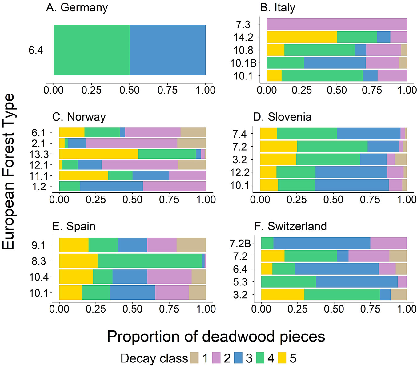
Deadwood measurements also included species and degree of decay ([34]): (i) bark intact, small branches present, wood texture intact; (ii) bark intact, no twigs; (iii) trace of bark, no twigs, hardwood texture with large pieces; (iv) no bark, no twigs, soft wood texture with blocky pieces; and (v) no bark present, no twigs, softwood with a powdery texture. We also mapped the position of the deadwood pieces. The deadwood protocol also allows deadwood data to be recorded in a quarter of the plot (25 × 25 m) when the amount of deadwood was very large.
Deadwood was collected in one plot in Germany, five in Italy, six in Norway, five in Slovenia, five in Spain, and five in Switzerland. In the case of Germany, Switzerland, and forest type 10.1 in Italy, deadwood was only recorded in a quarter of the plot.
Bird and mammal diversity
Two surveys for vertebrate animals were proposed as optional measurements. The first was focused on birds and consisted of installing an audio recorder (Song Meter Micro and SM4 TS Wildlife Acoustics, Inc.) at the center of the plot. We planned to record bird singing over one month, spending two hours each day around sunrise and two hours around sunset, when bird activity is high ([17]). However, due to logistical constraints, these schedules varied across countries.
In Spain, Song Meter Micro bioacoustics recorders were installed in four forest types (8.3 Pyrenean oak, 10.1 Mediterranean pine forest, 10.4 Mediterranean and Anatolian Scots pine forests and 14.2 Plantations of non-site-native species and self-sown exotic forest) for one month during June-August 2023. The devices were programmed to record bird vocalizations for two hours around sunrise and two hours around sunset over one month.
In Norway, SM4 bioacoustics recorders were placed in five forest types for one week during June 2023: 2.1 (Hemiboreal forest), 6.1 (Lowland beech forest of southern Scandinavia and north-central Europe), 11.1 (Spruce mire forest), 12.1 (Riparian forest) and 13.3 (Mountain birch forest). The recording time schedule was the same as in Spain, two hours at sunrise and two hours at sunset over one month.
In Switzerland, Song Meter Micro bioacoustics recorders were installed in the two plots located in forest type 7.2 (Central European mountain beech forest). In the first of these plots (Forest type 7.2), the device was installed in July-August 2023. The recording time spanned one month and the device was scheduled to record for 30 minutes around sunrise and sunset. In the other plot (Forest type 7.2B), the devices were programmed to record bird vocalizations for 40 minutes around sunrise and 40 minutes around sunset over three weeks in August-September 2023.
Bird species were identified using the open-source deep learning algorithm BirdNET, enabling the geographic species filter ([38]). Each BirdNET detection has a confidence value ranging from 0 to 1. Values close to 1 indicate higher confidence that the sound record corresponds to the target species. Increasing the value of this parameter means higher precision and a reduction in the total number of species detected, i.e., a drop in false positives and an increase in false negatives ([62], [26]). For this pilot study, we used a confidence threshold of 0.7. The above authors also recommend filtering the species according to the number of BirdNET detections. In this study, we filtered out those species with fewer than five BirdNET detections during one month’s monitoring period. If the monitoring period was less than one month, the threshold was set at two. We calculated the bird species richness by plot (i.e., forest type) as the total number of species in the plot (α-diversity). To analyse the bird communities in more depth, we performed an NMDS with a Jaccard community dissimilarity distance matrix based on the absence/presence data.
The second survey aimed to monitor mammals using phototrapping cameras (Strike Force ProX 1080®, Browning, Morgan, UT, USA). For this purpose, five cameras spread across the plot were installed at relevant points for fauna monitoring, such as wildlife path tracks, close to browsed shrubs, trees with bark stripping damage, and groups of faeces or water bodies. We ensured that the camera traps covered as much of the plot area as possible without overlapping sampling zones of each one. Cameras were mounted at 0.5-1.0 m height on big trees to minimize shaking. Furthermore, we cleared ground vegetation within the first few meters to prevent the cameras from being triggered by moving plants in the wind. This sampling was only performed in Spain, in the same plots where the bioacoustics recorders were installed. The monitoring period also spanned one month. Mammals were identified by visual inspection of the images. We also calculated richness at the forest type level for mammal data, but the number of observations impeded performing the NMDS analyses.
Results
Forest structural indices
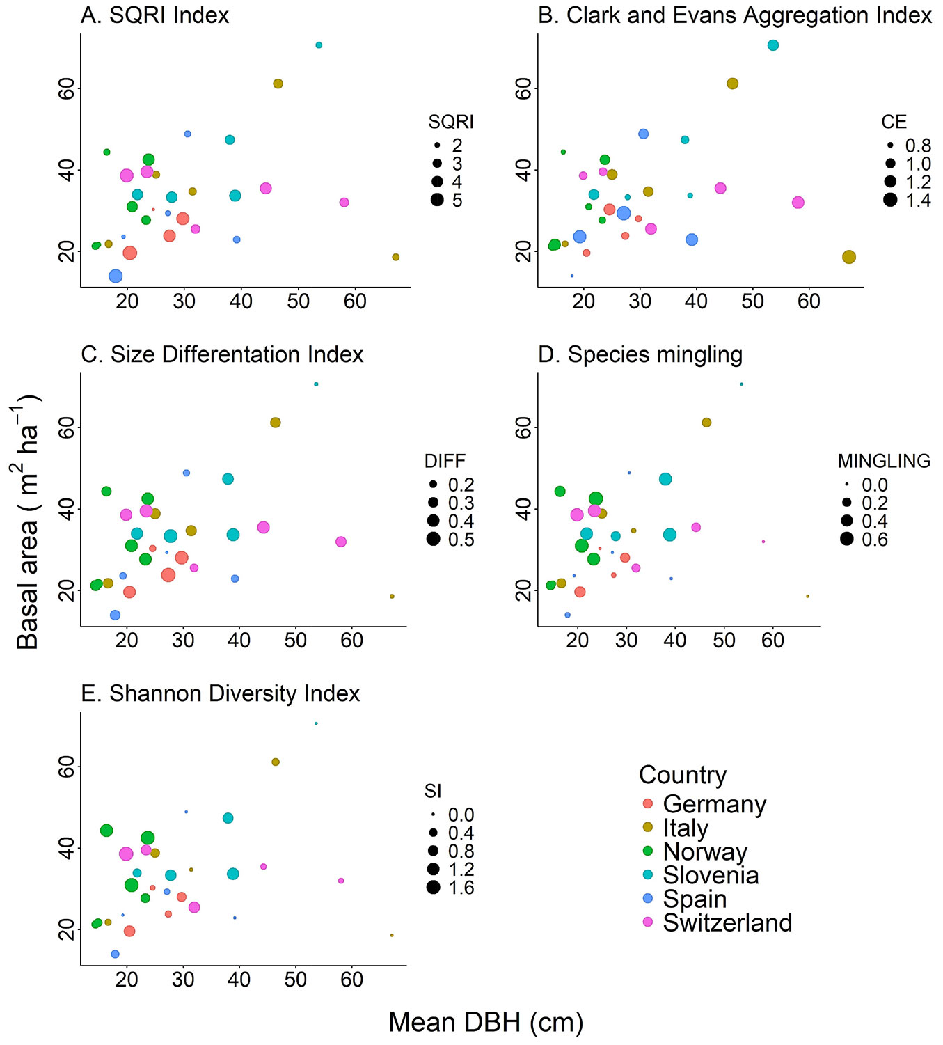
For each structural index, we found high variability between the forest types (Fig. 3). SQRI, the index related to forest complexity, ranged from 1.8 to 5.8 with a mean value of 3.5. CE, which is associated with the spatial pattern of trees, ranged from 0.7 to 1.4 with a mean value of 1.0. DIFF, the size differentiation index, ranged from 1.8 to 5.8 with a mean value of 3.5. Finally, the two indices for species composition (MINGLING and SI) presented values equal to zero in single-species forests. The mean value for MINGLING was 0.2 and the maximum was 0.7, while the mean for SI was 0.5 and the highest was 1.7.
Fig. 3 - Relationships among plot basal area, plot mean diameter at breast height and the five structural indices by country. Every point represents a plot (n = 30). Note that the value of the Species mingling (MINGLING) and Shannon Diversity Index (SI) is zero when only one species occurs in the plot. (SQRI): Square Root of Differences Index; (CE): Clark and Evans Aggregation Index; (DIFF): Size Differentiation Index.
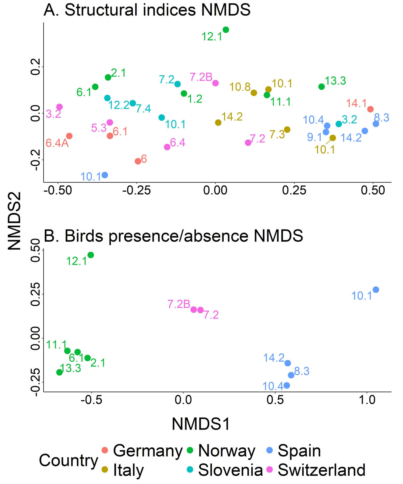
The stress statistic was 0.06, indicating that the data is well-represented in the reduced space. Overall, forest types from the same country tended to group closely together, with some exceptions, such as forest type 10.1 in Spain and 14.1 in Germany (Fig. 4A). This suggests that forest types located near each other in the reduced space shared similar structural characteristics. In contrast, the Norwegian data were not clustered together but were spread across the upper part of the reduced space. Additionally, plots from Mediterranean countries (Italy and Spain) were predominantly situated on the right side of the panel, while observations from Northern and Central European countries were more frequently found toward the center and left side.
Fig. 4 - Non-metric Multidimensional Scaling (NMDS) for the structural indices (A) and bird presence/absence data. NMDS1 and NMDS2 refer to the reduced dimension of the data. Points represent the European Forest Types as defined by Barbati et al. ([6]) and colours the countries.
Forest regeneration
Regeneration was present in all plots except for four forest types in Spain (8.3, 9.1, 10.4 and 14.2 - Tab. 1). We found recruits of 17 species distributed across the monitored plots. The Swiss plots located in forest types 6.4 and 7.2 accounted for the largest number of saplings with more than 10.000 recruits per ha of Fagus sylvatica L. (Fig. 5A). Regarding the seedlings, forest type 10.1 had the largest number of seedlings (about 8.000 seedlings per ha of Fraxinus ornus L. - Fig. 5B)
Deadwood
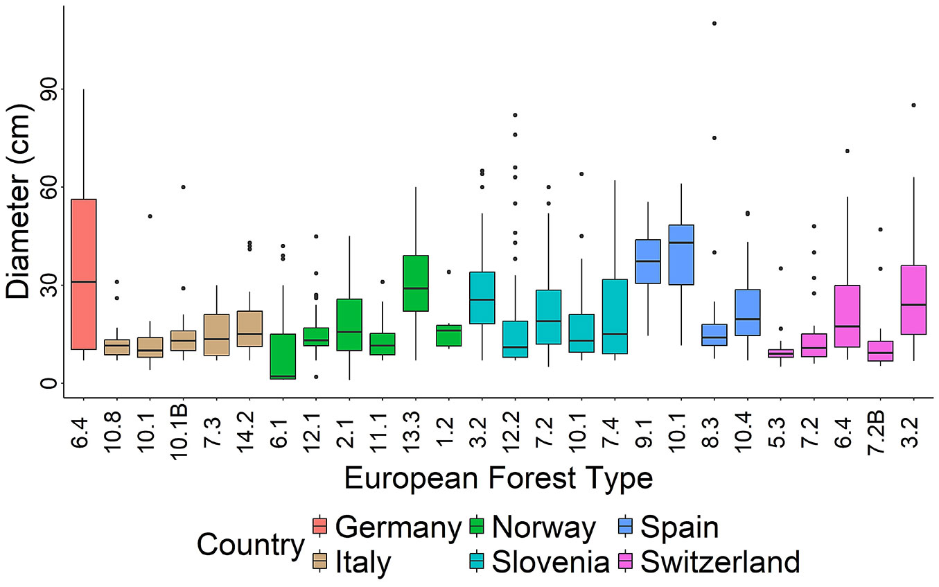
Fig. 6shows the distribution of deadwood pieces by size and forest type. The highest median values for deadwood, exceeding 40 cm, were observed in forest type 10.1 (Thermophilous pine forest). In contrast, the lowest median values were found in forest type 6.1 (Lowland beech forest of southern Scandinavia and north-central Europe). The number of deadwood pieces varied significantly among forest types, peaking at 166 records in forest type 7.4 (Illyrian mountainous beech forest, Slovenia). In contrast, the minimum of zero records meeting the sampling criteria was found in forest type 14.2 (Plantations of non-site-native species and self-sown exotic forests, Spain).
Fig. 6 - Boxplot of the deadwood pieces according to their diameter by European Forest Types (axis x) as defined by Barbati et al. ([6]) (see Tab. 1) and country (represented by filled colors). Note that the data from Germany, Switzerland and forest type 10.1 in Italy were only collected in a quarter of the plot and in one Spanish plot (forest type 14.2) there was no deadwood meeting the established criteria.
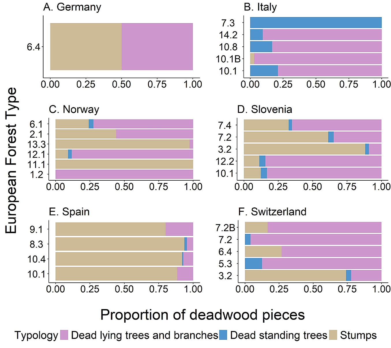
Regarding the degree of decay, pieces with moderate decay status (classes 2-4) were the most common in most forest types (Fig. 7). Lying deadwood (i.e., lying trees and branches) and stumps were the most common types of deadwood across the monitored plots, while the number of standing dead trees was negligible (Fig. 8).
Bird and mammal diversity
In Spain, the song recordings for each forest site reached around 20 GB and were stored in “.wav” format. After applying the filters described above, BirdNET identified 21 bird species in forest type 8.3, 33 in forest type 10.1, 18 in forest type 10.4, and 32 in forest type 14.2 (see Tab. S1 in Supplementary material for the complete list of species). For forest type 8.3, the families Fringillidae, Muscicapidae, Paridae, and Picidae accounted for the highest number of bird species, with two species per family. Fringillidae (n = 4 bird species), Corvidae (n = 3), and Paridae (n = 3) were the families with the largest number of bird species in forest type 10.1. Similarly, Fringillidae and Paridae were the families most represented in terms of number of bird species in the case of forest type 10.4. Finally, for forest type 14.2, Paridae (n = 3), Columbidae (n = 2), Corvidae (n = 2), Fringillidae (n = 2), Picidae (n = 2), Rallidae (n = 2), Scolopacidae (n = 2) and Turdidae (n = 2) accounted for the largest number of bird species.
In the case of Norway, BirdNET detected 42 bird species in forest type 12.1, 38 in forest types 13.3, 2.1, and 6.1, while 37 bird species were detected in forest type 11.1 (see Tab. S1 in Supplementary material). In forest type 12.1, Fringillidae (n=4 bird species), Picidae, Scolopacidae, and Turdidae (n=3) were the most represented families. Similarly, Fringillidae (n = 5), Turdidae (n=4), Muscicapidae and Scolopacidae (n = 3) were the predominant families in terms of number of bird species in forest types 13.3. For forest type 11.1, Fringillidae (n = 6) was the predominant family, followed by Turdidae (n = 5), Corvidae, and Paridae (n = 3). In the case of forest type 2.1, Fringillidae and Turdidae, with four species, were the most represented families. Finally, Picidae, Fringillidae, and Picidae, with four species each, were the families with the largest number of species in forest type 6.1.
In Switzerland, BirdNET identified 38 (Forest type 7.2B) and 48 (Forest type 7.2). Muscicapidae (n = 5) and Picidae (n = 4) were the most represented families in the first plot, while Muscicapidae (n = 5), Corvidae (n=4), and Picidae (n=4) were the predominant families in the other plot.
Regarding the NMDS analysis, the stress value was 0.04, below the threshold of 0.2, indicating a good data representation. Norwegian forest types were clustered on the left side of the reduced space, except for forest type 12.1 (Fig. 4B), while Swiss forest types were located at the center, and Spanish forest types appeared on the right side. This indicates that the bird communities studied had large inter-country variability but low intra-country variability. As regards the mammal survey in Spain, the number of photos varied widely among cameras (from 29 to 7.892 photos) and forest types (from 1.318 to 10.371 photos). We identified the following six species in forest type 8.3: wild boar (Sus scrofa L., family Suidae), rabbit (Oryctolagus cuniculus L., family Leporidae), roe deer (Capreolus capreolus L., family Cervidae), red fox (Vulpes vulpes L., family Canidae), common genet (Genetta genetta L., family Viverridae), beech marten (Martes foina Erxleben, Mustelidae) and some micromammals. In the case of forest type 10.1, we captured the following seven species of mammals: roe deer, wild boar, beech marten, common genet, Iberian hare (Lepus granatensis Rosenhauer, family Leporidae), European badger (Meles meles L., family Mustelidae) and European wildcat (Felis silvestris Schreber, family Felidae). The cameras recorded images of these six species of mammals in forest type 10.4.: roe deer, wild boar, European wildcat, beech marten, red fox, and European badger. Finally, in forest type 14.2, we found these six mammal species: roe deer, wild boar, red fox, European fallow deer (Dama dama L., family Cervidae), beech marten, and European wildcat. Overall, Cervidae, Leporidae, and Mustelidae, with two species, were the most represented families in the Spanish plots. Furthermore, the cameras captured domestic cows, dogs, and some birds in most of the forest types.
Discussion
The new EU forest strategy for 2030 emphasizes that forests are rich in biodiversity and play a crucial role in the fight against climate change. However, biodiversity-related variables vary significantly among European NFIs and other large-scale monitoring networks. While traditional measurements such as dendrometric data and deadwood assessments are common, information on other life forms, including fungi, mammals, birds, and invertebrates, is often limited ([14]). In this work, we reviewed the utility of traditional measurements and proposed new measurements to monitor biodiversity in forest inventories.
Given biodiversity’s broad and complex nature, several authors have emphasized the need for a consistent and statistically rigorous monitoring program capable of assessing its status and tracking changes over time and space. Such a program should be based on large-scale networks and well-defined indicators. Additionally, since the demand for information on forest biodiversity continues to grow, obtaining comparable, large-scale results is crucial to address challenges related to climate change and biodiversity loss. However, biodiversity data inherently rely on field-based measurements, which are often expensive to collect and difficult to compare when initial definitions or field protocols vary. In this context, where multiple forest inventories are expanding data collection efforts to meet new national and international requirements, developing a standardized framework for new variables and harmonizing existing ones is a timely and valuable opportunity. These advancements would significantly improve the quality and comparability of biodiversity data, fostering a deeper understanding of forest ecosystems and their dynamics.
Biorecorders and deep learning provide a reasonably accurate representation of the bird communities ([26]). Furthermore, the location and the recording time are saved in audio files that can be stored in open-access repositories for further analyses at broader spatio-temporal scales ([69]), using improved algorithms for external double-checking. Hence, they could potentially be used to meet indicator 4.10 (“Common bird species”) in the State of Europe’s Forests report ([22]). Currently, this information is provided by the Pan-European Common Bird Monitoring Scheme ([57]). However, this data cannot be directly linked to forest attributes such as forest structure.
The main drawbacks associated with employing these devices to monitor bird and mammal diversity in extensive monitoring programs such as NFIs or ICP plots are the human, economic, legal, and biological constraints. First, field crews must visit the same plot twice (once to install and once to retrieve the device), which could affect their efficiency and increase the overall costs. Although the cost of biorecorders and phototrapping cameras has fallen in recent years, an extensive monitoring program requires many devices. Moreover, the installation and retrieval of the monitoring devices can easily be performed without the need of experts. In this study, we used five phototrapping cameras per forest type, though their number should be reduced for biodiversity inventories at broader spatial scales. Additionally, since the monitoring period should be brief, the devices can be reused across different plots. It is important to note that these devices are at risk of theft or vandalism, which also implies increased costs. Finally, capturing photos and audio may infringe privacy rights in certain cases, thus requiring additional permission ([23]).
The total number of bird and mammal species at a given sampling point is affected by several constraints, the phenological and physiological behaviour of the animals being among the main ones. For instance, some mammals such as bears hibernate, while migration is common in many avian species ([21], [73]). Therefore, species richness is modulated to some extent by the monitoring period. This shortcoming could be addressed by increasing the monitoring periods, though this involves the plots being revisited to change batteries, download the data, or change the memory cards. For further weaknesses and shortcomings and the accuracy of BirdNET, refer to Pérez-Granados ([62]).
Regarding the photo trapping, the images captured were visually inspected. However, several options for image processing and automatic identification of species are available, such as camtrapR ([50]) or Agouti ([1]), as well as others based on citizen science ([30]), which may facilitate data management. Similar to bird singing records, mammal photos recorded with cameras can also be stored in public repositories for further analysis. Alternative methods for mammal monitoring include faeces recognition, the identification of tracks on the ground, trapping, or bark rubbing ([74]). Some of these methods require high qualification of the field crews (e.g., faeces recognition or track identification) or can be restricted to some species (e.g., bark rubbing for deer and similar species), while trapping is not a feasible procedure for broad-scale surveys.
Bat species have been proposed as bioindicators, and their monitoring is compulsory according to the 92/43/EEC “Habitats” Directive. This taxonomic group could be restricted by sampling limitations, taxonomic issues, or geographical constraints ([66]). However, bird monitoring devices have modules or configuration settings specifically designed for bat recordings ([25]).
In this study, we also analyzed other well-known components of biodiversity, such as forest structure and deadwood. We quantified forest structure using non-spatially explicit indices and nearest neighbour indices that can be easily computed and provide a wide representation of the forest structure. Other alternatives are available beyond the nearest neighbour indices, such as second-order moment functions (e.g., Ripley’s K and related functions). Regardless of the index used, the reliability of the index is conditioned by the plot design. For instance, plots that are too small do not capture the spatial pattern of the trees, while concentric/nested designs require specific methodologies for adequate index estimation ([46]). These circumstances are challenges in reporting forest information and comparing forest structures with different plot designs across countries.
As regards the deadwood indicator, we used fixed area sampling, i.e., we measured all the pieces that met the size criteria in a given area. We also recorded the degree of decomposition as this measure is easily collected in the field and provides insights into habitat suitability for different species ([54]). However, we did not record the height of the dead trees, which limits the calculation of volume and biomass stocks. In this pilot study, we propose surveying the whole plot or a quarter of the plot area, depending on site conditions and deadwood accumulation. For extensive monitoring surveys, measuring all the deadwood pieces in the plot is unrealistic, given the human and economic constraints involved. Hence, deadwood measurements can be restricted to subplots nested within the plot, as in the Spanish NFI. Alternatively, the linear intercept technique may be employed to measure lying deadwood (coarse woody debris). In this regard, many studies deal with the performance, weaknesses, and strengths of the alternative methods for sampling deadwood ([64]). Furthermore, some NFIs (e.g., Spain) record deadwood data in a subsample of the complete array of plots to reduce sampling efforts ([3]).
Tree species richness (the number of tree species in a given area - [10]), is an essential measure for quantifying forest diversity in forest ecosystems. Nonetheless, it is somewhat influenced by the design and size of the plot, as well as the sample size ([60], [47]). Beyond tree richness, it is also important to understand the degree of intra-species variability so that adequate management of genetic resources and adaptive strategies to mitigate the effects of climate change can be implemented ([27], [53]). This requires the collection of plant material to be analyzed by genetic markers, such as neutral and adaptive Single Nucleotide Polymorphisms (SNPs - [53]). However, the collection of plant material (typically leaves, needles, or seeds, though seedlings can also be sampled) is constrained by the accessibility of the tree crown in adult stands. Some European NFIs have included these protocols either in a subsample or in the complete array of plots; however, to our knowledge, no scientific publications have included these data.
Another relevant source of biodiversity is the understory, which includes individuals of tree species below the minimum measurable size (regeneration cohorts), shrubs, herbs, grasses, ferns, and other life forms such as mosses or lichens. Regeneration, which is designated as biodiversity indicator 4.2 in the State of Europe’s Forests report, is essential for ensuring the continuity and renewal of forests. It has also been recognized as a vital reservoir of biodiversity because it supports many tree species that often do not reach the minimum threshold ([47]). In our case study, we split the regeneration into two cohorts (seedlings and saplings) measured in subplots located at the northernmost corner of the plot. Assessing regeneration in smaller subplots is a standard procedure in NFIs worldwide to reduce sampling efforts ([42]). In contrast to our approach, other NFI plot designs often position the regeneration subplot at the plot center or use a cluster of several regeneration subplots. Both methods have strengths and weaknesses ([14]). Clustering multiple subplots captures greater spatial variability in regeneration, but it also requires significantly more time during fieldwork. While efforts have been made to establish indicators for assessing regeneration to a broad extent, no definitive conclusions have been reached due to significant variability in regeneration definitions, sampling areas, and measurement protocols ([13]). Improving regeneration assessment is therefore crucial to enable meaningful comparisons across different regions.
Regarding other understory components, assessing shrub species and their abundance is a common task in NFIs ([14]), though taxonomy issues, such as difficulties in species identification, can hinder the evaluation of other taxa.
Finally, despite the major role of soil in biodiversity accounting ([75]), the carbon cycle ([43]) and the overall ecosystem functionality ([67]), we did not evaluate any aspects related to soil biodiversity. These measurements are expensive and require harmonized field and laboratory protocols. Ideally, the same laboratory should analyse all the samples.
Conclusions
To optimize human and economic resources, we suggest these new biodiversity measurements be undertaken in a subset (to ensure that it is affordable and logistically feasible) of NFI plots and/or ICP plots (Level I and II) covering the relevant forest types. This will provide valuable insights into in forest biodiversity assessment, their conservation, and the effect of management on their sustainability, thus improving the information and allowing better decision-making. Only with reliable and robust data are essential to effectively address the complex questions on the multifunctional role of the forests. However, it is worth noting that including specific protocols for birds and mammals may introduce logistical challenges. For example, monitoring plots may need to be visited twice during specific times of the year, which could differ from the standard procedures used by many extensive monitoring programs. Legal constraints must also be considered, as the locations of plots may need to be disclosed, and obtaining the necessary permissions to install monitoring devices could present administrative challenges.
Given the increasing international interest in biodiversity monitoring at large scales, we recommend: (i) fostering the harmonization process to ensure comparability of the different attributes from one country to another, as many potential biodiversity indicators are highly dependent on the area and the target variable (structure, dead wood, composition); (ii) establishing standardized and harmonized protocols for new biodiversity variables, using standard guidelines across countries that will facilitate spatio-temporal comparisons between local, national and international areas as well as the reporting to international agreements. Biodiversity indicators derived from these protocols can be valuable in establishing both forest management guidelines and silvicultural operations (e.g., delimitation of protective areas or promotion of specific forest structures) aimed to achieve biodiversity enrichment alongside other forest functions. Further analyses using larger datasets should evaluate the protocols’ performance and efficiency to identify potential improvements.
List of abbreviations
The following abbreviations have been used throughout the paper:
- CE: Clark and Evans index;
- dbh: diameter at breast height;
- DIFF: size differentiation index;
- ICP: International Co-operative Programme on Assessment and Monitoring of Air Pollution Effects on Forest;
- MINGL: species mingling index;
- NFI: National Forest Inventories;
- SI: Shannon’s Diversity Index;
- SRQI: sum of squared of differences index.
Acknowledgements
This work has been partly funded by the European Union Horizon Europe Research & Innovation programme, under the Grant Agreement no. 101056907 (PathFinder project). We acknowledge the effort made by everyone involved in the field data collection. We thank Lutz Fehrmann for his valuable inputs, Alejandro Rodríguez and Rafael Villafuerte-Jordán for their help in identifying some mammal species, and Adam Collins for revising the English grammar.
References
CrossRef | Gscholar
Gscholar
CrossRef | Gscholar
CrossRef | Gscholar
Gscholar
CrossRef | Gscholar
Gscholar
CrossRef | Gscholar
Online | Gscholar
CrossRef | Gscholar
CrossRef | Gscholar
CrossRef | Gscholar
CrossRef | Gscholar
Gscholar
Supplementary Material
Authors’ Info
Authors’ Affiliation
Isabel Cañellas 0000-0002-9716-7776
Iciar Alberdi 0000-0003-1338-8465
Institute of Forest Science of the National Institute for Agricultural and Food Research and Technology - INIA-CSIC (Spain)
Stefano Puliti 0000-0003-4624-8987
Norwegian Institute of Bioeconomy Research (NIBIO), Division of forest resources (Norway)
Giovanni D’Amico 0000-0002-2341-3268
Francesca Giannetti 0000-0002-4590-827x
Università degli Studi di Firenze (Italy)
Ross Shackleton 0000-0001-5628-4506
Swiss Federal Institute for Forest, Snow and Landscape Research - WSL (Switzerland)
Corresponding author
Paper Info
Citation
Moreno-Fernández D, Breidenbach J, Cañellas I, Chirici G, D’Amico G, Ferretti M, Giannetti F, Puliti S, Schnell S, Shackleton R, Skudnik M, Alberdi I (2025). Enhancing forest biodiversity indicators in inventories through harmonized protocols. iForest 18: 109-120. - doi: 10.3832/ifor4778-018
Academic Editor
Marco Borghetti
Paper history
Received: Dec 19, 2024
Accepted: Feb 03, 2025
First online: May 20, 2025
Publication Date: Jun 30, 2025
Publication Time: 3.53 months
Copyright Information
© SISEF - The Italian Society of Silviculture and Forest Ecology 2025
Open Access
This article is distributed under the terms of the Creative Commons Attribution-Non Commercial 4.0 International (https://creativecommons.org/licenses/by-nc/4.0/), which permits unrestricted use, distribution, and reproduction in any medium, provided you give appropriate credit to the original author(s) and the source, provide a link to the Creative Commons license, and indicate if changes were made.

Web Metrics
Breakdown by View Type
Article Usage
Total Article Views: 12001
(from publication date up to now)
Breakdown by View Type
HTML Page Views: 5999
Abstract Page Views: 3123
PDF Downloads: 2593
Citation/Reference Downloads: 9
XML Downloads: 277
Web Metrics
Days since publication: 418
Overall contacts: 12001
Avg. contacts per week: 200.97
Article Citations
Article citations are based on data periodically collected from the Clarivate Web of Science web site
(last update: Mar 2025)
(No citations were found up to date. Please come back later)
Publication Metrics
by Dimensions ©
Articles citing this article
List of the papers citing this article based on CrossRef Cited-by.
Related Contents
iForest Similar Articles
Research Articles
Towards harmonization of forest deposition collectors - case study of comparing collector designs
vol. 4, pp. 218-225 (online: 03 November 2011)
Commentaries & Perspectives
Harmonizing forest inventories and forest condition monitoring - the rise or the fall of harmonized forest condition monitoring in Europe?
vol. 3, pp. 1-4 (online: 22 January 2010)
Research Articles
Bird composition and diversity in oak stands under variable coppice management in Northwestern Turkey
vol. 11, pp. 58-63 (online: 25 January 2018)
Review Papers
Biodiversity assessment in forests - from genetic diversity to landscape diversity
vol. 2, pp. 1-3 (online: 21 January 2009)
Research Articles
Long-term outcome of precommercial thinning on floristic diversity in north western New Brunswick, Canada
vol. 1, pp. 145-156 (online: 25 November 2008)
Research Articles
Effects of different silvicultural measures on plant diversity - the case of the Illyrian Fagus sylvatica habitat type (Natura 2000)
vol. 9, pp. 318-324 (online: 22 October 2015)
Commentaries & Perspectives
Key information for forest policy decision-making - Does current reporting on forests and forestry reflect forest discourses?
vol. 16, pp. 325-333 (online: 15 November 2023)
Research Articles
The effects of forest management on biodiversity in the Czech Republic: an overview of biologists’ opinions
vol. 15, pp. 187-196 (online: 19 May 2022)
Research Articles
Investigating the effect of selective logging on tree biodiversity and structure of the tropical forests of Papua New Guinea
vol. 9, pp. 475-482 (online: 25 January 2016)
Research Articles
Diversity of saproxylic beetle communities in chestnut agroforestry systems
vol. 13, pp. 456-465 (online: 07 October 2020)
iForest Database Search
Search By Author
- D Moreno-Fernández
- J Breidenbach
- I Cañellas
- G Chirici
- G D’Amico
- M Ferretti
- F Giannetti
- S Puliti
- S Schnell
- R Shackleton
- M Skudnik
- I Alberdi
Search By Keyword
Google Scholar Search
Citing Articles
Search By Author
- D Moreno-Fernández
- J Breidenbach
- I Cañellas
- G Chirici
- G D’Amico
- M Ferretti
- F Giannetti
- S Puliti
- S Schnell
- R Shackleton
- M Skudnik
- I Alberdi
Search By Keywords
PubMed Search
Search By Author
- D Moreno-Fernández
- J Breidenbach
- I Cañellas
- G Chirici
- G D’Amico
- M Ferretti
- F Giannetti
- S Puliti
- S Schnell
- R Shackleton
- M Skudnik
- I Alberdi
Search By Keyword


