Introduction 

A forest is a three-dimensional ecosystem, and its structure can vary in both the vertical and horizontal directions. The horizontal distribution pattern of trees has always been a research hotspot. It is believed to be directly related to ecological processes within the forest community (e.g., seed dispersion, regeneration, death, resource utilization, and gap formation - [39], [25]), and strongly influences tree growth and timber yield ([6]). In contrast, vertical structure has not attracted much attention. This may be because the vertical structure is difficult to measure directly and the results are difficult to apply in practice. However, several studies have indicated that vertical structure plays an important role in forest ecosystems ([11], [8]). It affects the forest dynamics and modifies the supply, capture, and efficiency of use of resources, and thus also inter- and intra-specific interactions ([6]). It is also closely related to the ability of a forest stand to resist external non-biological interference, and the number and species of wild animals living in the forest ([17]).

Vertical stratification of trees is an important phenomenon in natural forests ([13]). The upstory constitutes the skeleton of the forest community. A change of canopy structure in the horizontal and vertical directions leads to the formation of a complex light and shade structure in the understory ([10]), determining the species composition, distribution pattern, and ecological processes in the understory. Illumination may be the most readily available resource for understory ([22]). When seedlings are successfully renewed and escape competition from the groundcover, light often becomes a key factor for the survival and growth of young trees in the understory ([26]). Through canopy interference, the upstory will increase the variability and heterogeneity of understory resources, and change the internal rainfall distribution and quantity ([26]), soil properties (soil organic matter, available N, cation exchange capacity, litter thickness, soil calcium content, humidity, temperature, pH, and frost - [3]), and litter decomposition ([8]). This in turn affects the productivity and diversity of understory ([10]). In addition, the canopy density of the upstory also affects the seed distribution of understory and upstory in the forest and the seed bank composition ([34]).

The understory may also affect regeneration, seedling growth, and forest dynamics by changing the soil seed bank, invading and occupying forest gaps, which will eventually have an impact on the upstory structure and species composition ([34], [10]). In both tropical and temperate regions, the interaction between upstory and understory is considered to be an important factor determining the structure and dynamics of forest communities ([34]). However, the relationship between upstory and understory is not fully understood ([2]). Most studies of the spatial structure of forest communities consider the species comprising the community as a whole ([12], [4]), while others have analyzed the spatial correlation of the different life histories of single populations or several groups of the same genus ([11], [44], [25]). Still other studies have focused on tree groups that belong to certain synusia or growth stages, such as seedlings and small trees ([5]), or dominant trees ([35], [9]). Elsewhere, the spatial association between specific objects, such as dead trees and living organisms, have been considered ([32], [40]), in addition to regeneration and dead wood or earthen mounds ([14]). However, few studies have stratified forest communities and considered each layer as a separate part, especially at the meso-scale ([8]). Each layer may have different growth or distribution pattern characteristics, providing valuable clues for investigations of the mechanisms by which species coexist.

The species composition of forests in temperate regions is relatively simple and, due to the particular renewal and growth characteristics of some species (e.g., “wave”, “stop-and-go”, or “continuous and fast growing” strategies - [11]), vertical stratification is common ([8], [35], [9], [25]). However, in tropical South Asia, there is an abundance of species components and a continuous distribution of species in the vertical direction can readily occur. Many climbing vines may also be attached to trees ([42]), which further influences the vertical stratification of the forest community. In addition, the “slash-and-burn” agricultural management model was widely practiced in the region. This destroyed large amounts of primary vegetation, resulting in a complex composition and structure of secondary forests ([40]). The mixed pine-oak forest along the Nanpan River in southwest China is a typical example; it is a secondary forest that developed after the original forest suffered clear cutting in 1960s and was then completely abandoned and left unused. After self-development, it formed a forest that mainly consists of Pinus yunnanensis var. tenuifolia and several species of Quercus ([21]). It is currently in the early stage of succession with high species diversity, but vertical stratification is very obvious. This provides a good opportunity to study the construction of secondary forest structure after disturbance.

The purpose of this study was: (1) to identify the distribution pattern and spatial correlation of trees in the early stages of a secondary forest; and (2) to determine the spatial distribution of tree species and tree size in the vertical layers of the forest.

  Material and methods 

Study area and field measurements

The study site was located in Yachang Township, Leye County, Baise City, Guangxi Zhuang Autonomous Region (Fig. S1 in Supplementary material). The Nanpan River, which originates in Yunnan Province, separates Guangxi and Guizhou provinces as it passes through this region. The southern part of Guangxi Zhuang Autonomous Region has a typical karst landform, with limestone as the main rock type, but there are also some large mountains comprised of weathered rock. Historically, the majority of the township was part of the state-owned Yachang Forest Farm, which was later renamed the Guangxi Yaychang National Orchid Reserve due to the depletion of forest resources, together with the existence of a large number of wild orchid communities and the natural landscape of the “Tiankeng Group”. Temperature, soil types, and rainfall in the region vary dramatically with elevation and geomorphology ([18]). The river valley has a relatively high temperature and long hot summers. Its average temperature in July is 28.4 °C, with an extreme high temperature of 42.5 °C (historical record since 1981). There is no frost and snow in winter. The average annual rainfall is 800 mm, but the distribution is extremely uneven. Summers are wet, but spring and autumn are rainless and seasonal droughts can occur. The soil type gradually transitions from cinnamon soil in the river valley to cinnamon red soil in the mountain plain and a yellow soil in the mountains. The soil is generally barren, with a high gravel content ([21], [41]).

The sample site was located on a mud hill, 20 km from the administrative center of Yachang township. The elevation was about 760 m a.s.l. and the study site was about 250 m from the river. The forest stand was divided into two vertical layers. The upper layer mainly contained P. yunnanensis, Quercus variabilis Bl. and Albizzia kalkora (Roxb.) Prain, while the lower layer was dominated by Vaccinium bracteatum Thunb., Phyllanthus emblica L., Wendlandia uvariifolia Hance, Craibiodendron stellatum (Pierre) W. W. Smith, Ardisia quinquegona Bl., and Toona ciliata M. Roem. Some orchids were present in the stand, including Dendrobium officinale Kimura & Migo, Cleisostoma fuerstenbergianum Kraenzl., Vanda concolor Bl. and Cymbidiumensifolium (L.) Sw. Other herbs in the stand included Thysanolaena maxima (Roxb.) Kuntze and Miscanthus floridulus (Lab.) Warb. ex Schum et Laut (Fig. S2 in Supplementary material). Because it was situated in a mountainous location far from residential areas, the secondary forest had suffered almost no external interference, although some of the P. yunnanensis were scarified for sap in 1990a ([21]).

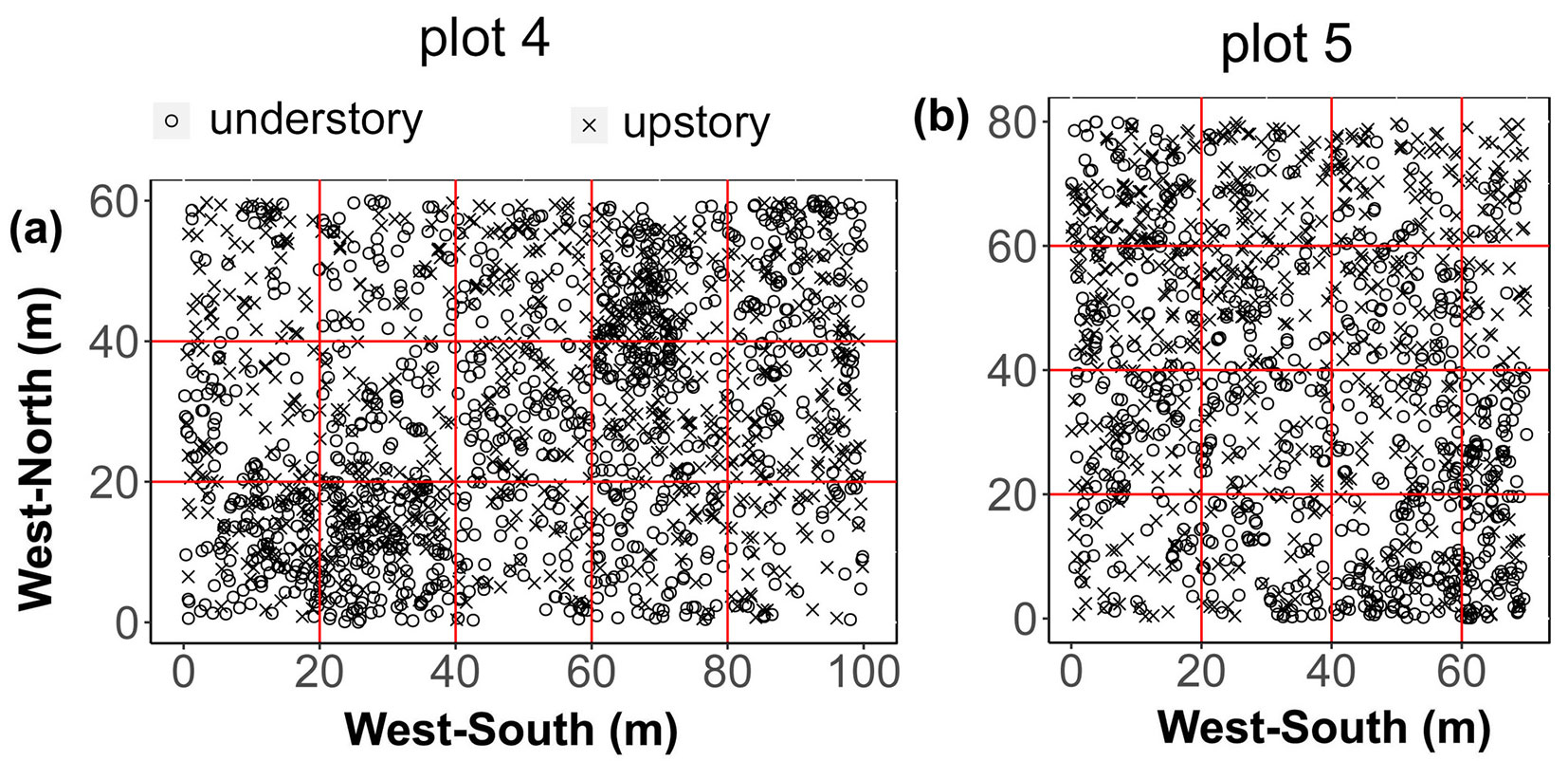
We established two rectangular standard plots (plot 4: 100 m × 60 m, up-slope, 106° 19’ 20" N, 24° 51’ 15.95" E; plot 5: 80 m × 70 m, mid-slope, 106° 14’ 9.5" N, 24° 27’ 28.9" E) in 2016-2018. The two sample sites were approximately 120 m apart, and had similar vegetation components. First, we divided each area into several subplots (20 × 20 m each) and determined the location of each living tree, standing dead trees, and fallen dead wood using a total station instrument (Southern Mapping Company, Johannesburg, South Africa - precision is 2mm + 2ppm). We measured all stems with at least 1 cm DBH. Then, we measured the tree height, DBH, and crown width of all standing trees. We also recorded species name and marked each living individual with a unique reference number. For fallen trees, the grade of decay (i-v), length of branches, and size of both ends were measured and recorded (Fig. 1). The diversity of herbs was determined using a systematic sampling method. We surveyed 26 and 27 tree species, 1745 and 1319 living trees, and 265 and 168 dead trees in plots 4 and 5, respectively. However, we only used the data of living trees which include all species for analysis.

Fig. 1 - Distribution of trees species in the sampling plots (a: plot 4; b: plot 5). Rings and crosses represent the locations of understory and upstory plants, respectively.

  Enlarge/Shrink   Download   Full Width  Open in Viewer

Data analysis

Classification of stratification

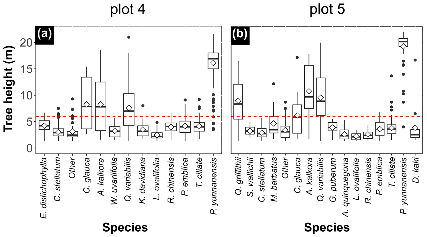
Tree height is a particularly important index of vertical structure and can be used to describe the stand ([6]). Vertical stratification in this study was determined according to the height of the lower layer; a box graph of the tree height of the two forests showed that the height of the lower layer was slightly more than 6 m (red dashed line in Fig. 2 - see also Fig. S2 in Supplementary material). Most lower layer plants were shrub species, accounting for 55.58 and 53.44% of the total number of stand plants and 84.61 and 89.47% of the overall populations in plots 4 and 5, respectively (Tab. S1). The understory also included some newly settled tree species that were still small (e.g., T. ciliata, and Toxicodendron vernicifluum [Stokes] F. A. Barkl.). Four tree species Q. variabilis, P. yunnanensis, A. kalkora, and C. glauca occupied both the upper and lower layers, but were dominant in the upper layer (Fig. 2). The C. glauca population only had 21 and 19 individuals in plots 4 and 5, respectively.

Fig. 2 - Tree height distribution in the vertical layers of the forest in both plots (plot 4, a; plot 5, b). The boundary of the vertical layers was close to 6 m. The understory mainly consisted of shrubs and a few tree species, while the upstory was dominated by several tree species. In plot 4, the proportion of the number and population for understory and upstory were 55.58%:44.42% and 84.61%:15.39%, respectively, and they were 53.44%:46.56% and 89.47%:10.53% in plot 5.

  Enlarge/Shrink   Download   Full Width  Open in Viewer

Spatial pattern analysis

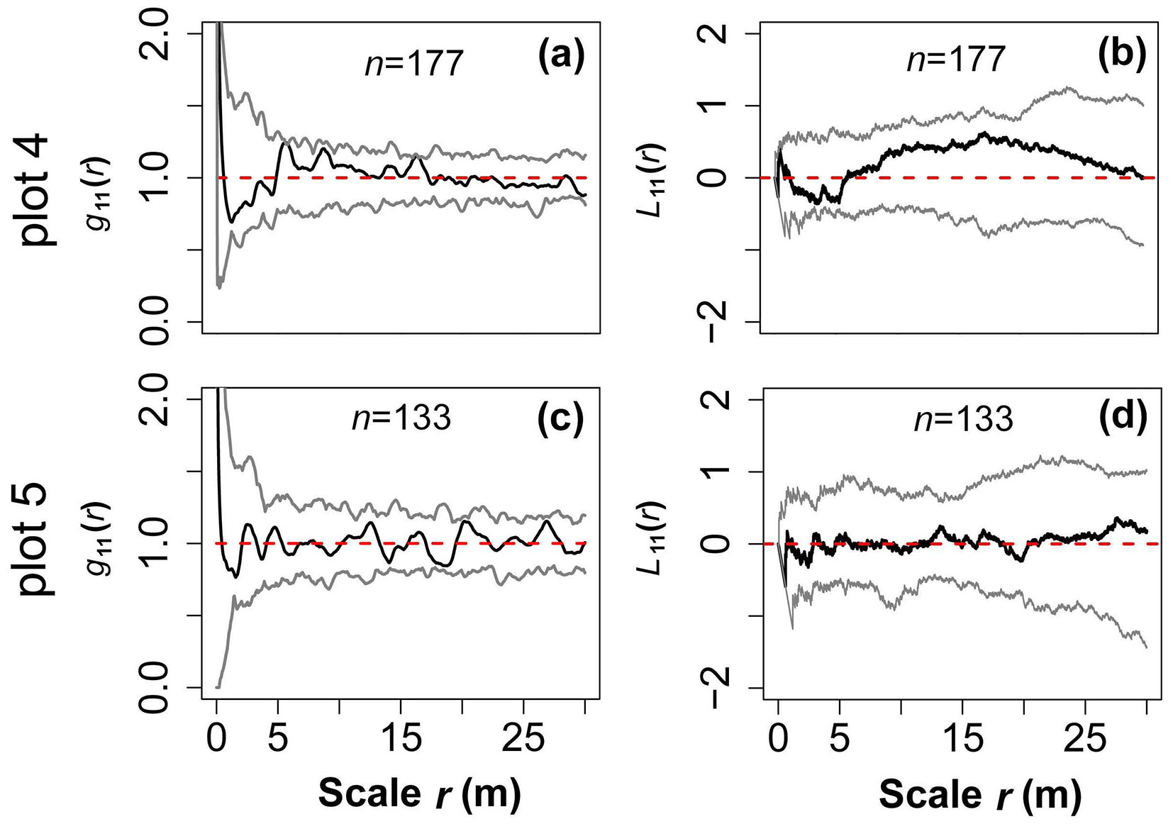
Fig. 3 - A pair correction function (PCF) and Lest heterogeneity test based on the null model of complete spatial randomness (CSR), indicating no significant heterogeneity in either forest stand. The red dashed lines are theoretical values, and the grey lines denote the 95% confidence limits of a Monte Carlo (MC) simulation. The black solid lines represent observed values and n is the number of large trees (DBH ≥ 20 cm) used to test heterogeneity.

  Enlarge/Shrink   Download   Full Width  Open in Viewer

A pair correction function (PCF), g(r), based on the paired point distance was used for spatial pattern analysis (eqn. 1). The g(r) is an improved model of the k-function (eqn. 3), which not only eliminates the statistical cumulative error of the k-function, but also makes the distribution pattern easier to understand with a change of scale ([11], [39], [4], [23]). It includes univariate distribution g₁₁(r) and bivariate distribution g₁₂(r) models. To ensure the correct use of the two models, it is necessary to know whether the sample site has a first-order effect caused by habitat heterogeneity (HP - [28], [39]). We therefore analyzed the distribution pattern of large trees (DBH ≥ 20 cm) on a relatively large scale (to limit the edge effect, r= 0-30 m, should be less than 1/2 the length of the smallest plot boundary) using g₁₁(r) and L₁₁(r) based on the null model of complete spatial randomness (CSR). L₁₁(r) (Lest) eliminates instability due to variance of the k-function, and is not very sensitive to changes in the distribution pattern at a small scale, being better able to reflect changes on a large scale (eqn. 3). In contrast, g₁₁(r) is very sensitive to changes in the distribution pattern on a small scale ([39]). The results showed that there was no habitat heterogeneity in either forest (Fig. 3). To explore the biological interactions among trees, the spatial distribution of the community, upper layer, and lower layer on a slightly smaller scale (r = 20 m) was analyzed based on the null model of CSR g₁₁(r). We used g₁₂(r) to analyze the spatial correlation between the upper and lower layers, and the spatial correlation among their main populations (n ≥ 40) based on a null model of the independence of components (eqn. 1, eqn. 2, eqn. 3).

where N is the number of trees, r is the radius, w_ij is the edge-correction weighting, and A is the area of sample.

Spatial distribution of species and sizes

Tree species and size differentiation are also closely related to scale ([12], [9]). In this study, we used Stoyan’s generalized model k_f (r) of the mark correlation function (MCF) based on a point process, X, to analyze changes in tree species and DBH with changes in the observation scale (eqn. 4). The k_f (r) is very flexible and can measure the spatial correlation of the mark of the i^th and j^th neighbors at a distance r. The mark used could be one of several classification variables (tree species in this study) or numeric variables (DBH in this study). An arbitrary f is often used to test the k_f (r) function. It has two parameters (m₁ and m₂), which are the corresponding possible marks. When the mark is DBH, f (m₁, m₂) = m₁ × m₂, and when tree species are the mark, f (m₁, m₂) = 1(m₁ = m₂). In eqn. 4, E_ij is the conditional expected value of the i^th and j^th trees at distance r in the point process X, and M(i) and M(j) are the marks attached to the i^th and j^th trees. In the denominator, M and M’ are random markers independently drawn from the edge distribution of the mark, and E is the common expected value. When the mark is attached to the point process X, it is independent and has the same distribution, k_f (r) = 1 (eqn. 4):

In the above analysis, the Monte Carlo (MC) method was used to randomly simulate the observation values of all observation scales 199 times, and the five maximum and five minimum values were obtained as the upper and lower 95% confidence intervals, enabling the significance of the deviation of the observed value from the theoretical value to be determined. For the spatial pattern, the g₁₁(r) theoretical value of a Poisson’s homogeneity test is 1 and the g₁₂(r) theoretical value is λ₂. An observed value outside the upper confidence limit indicated an aggregated distribution or positive association. An observed value falling outside the lower confidence limit indicated a regular distribution or negative association. An observed value within the envelope between the confidence intervals indicated a random distribution and random association ([23]). For the MCF, when calculating tree species, k_mm(r) = 1 means that tree species are independent from each other at the scale r, i.e., the probability that the neighbor j of any tree i is of the same species or a different species is equal. If k_mm(r) > 1 there is a positive correlation, i.e., conspecies aggregation or heterogeneity repulsion, and if k_mm(r) < 1 there is a negative correlation, i.e., heterogeneity aggregation or conspecies repulsion. For tree DBH, k_mm(r) = 1 indicates that the tree sizes at the scale r are independent from each other, and k_mm(r) > 1 indicates that the DBH of the two trees is positively correlated. If k_mm(r) < 1, the DBH of the two trees is considered to be negatively correlated, i.e., the DBH product of the two trees at the scale r is less than the mean DBH of all trees ([23]). The circle radius r simulated by the summary function was 20 m. For statistical convenience, when analyzing the spatial correlation between the main population of the upper layer and the main population of the lower layer, we set the distance of r to 1 m, while the distance for other analyses was 0.001 m. Data analysis and graphical processing were conducted in the “ggplot2” and “spatstat” packages of R ver. 3.25 (R Development Core Team, Vienna, Austria).

  Results 

Spatial patterns in the vertical layers

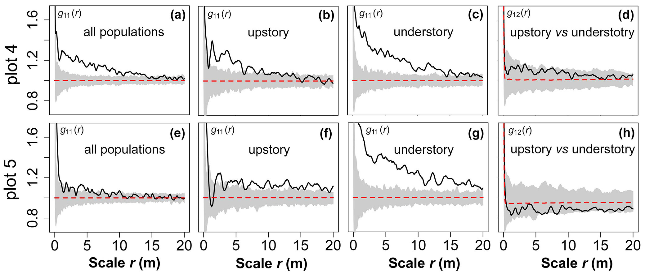
In plot 4, the clumped pattern of all populations extended for 14 m and then became a random distribution at larger scales (Fig. 4a). The distribution pattern of the upstory also gradually shifted from an aggregated to random distribution as the observation scale increased (Fig. 4b). Except for the random pattern at r = 18-20 m, the lower layer was aggregated at residual scales (r = 0-17 m - Fig. 4c). In addition, the upper and lower layers were randomly correlated at all scales (Fig. 4d). The trees in plot 5 were slightly aggregated at the medium and small scales (r = 0-10 m), but the distribution became random at a large scale (r = 10-20 m - Fig. 4e). The upper layer was close to a random distribution at small scales (r = 0-4 m), but at larger scales (r = 4-20 m) there was a low level of aggregation (Fig. 4f). The aggregation intensity of the understory was significantly higher than that of the upper layer (Fig. 4g), but the upper and lower layers were randomly correlated at all scales (r = 0-20 m - Fig. 4h).

Fig. 4 - Spatial distribution and spatial correlation of the upstory and understory in both plots. The grey background in each figure denotes the 95% confidence limits of an MC simulation. The black solid line represents the observed value and the red dashed lines are theoretical values.

  Enlarge/Shrink   Download   Full Width  Open in Viewer

Spatial correlation of the main populations in the vertical layers

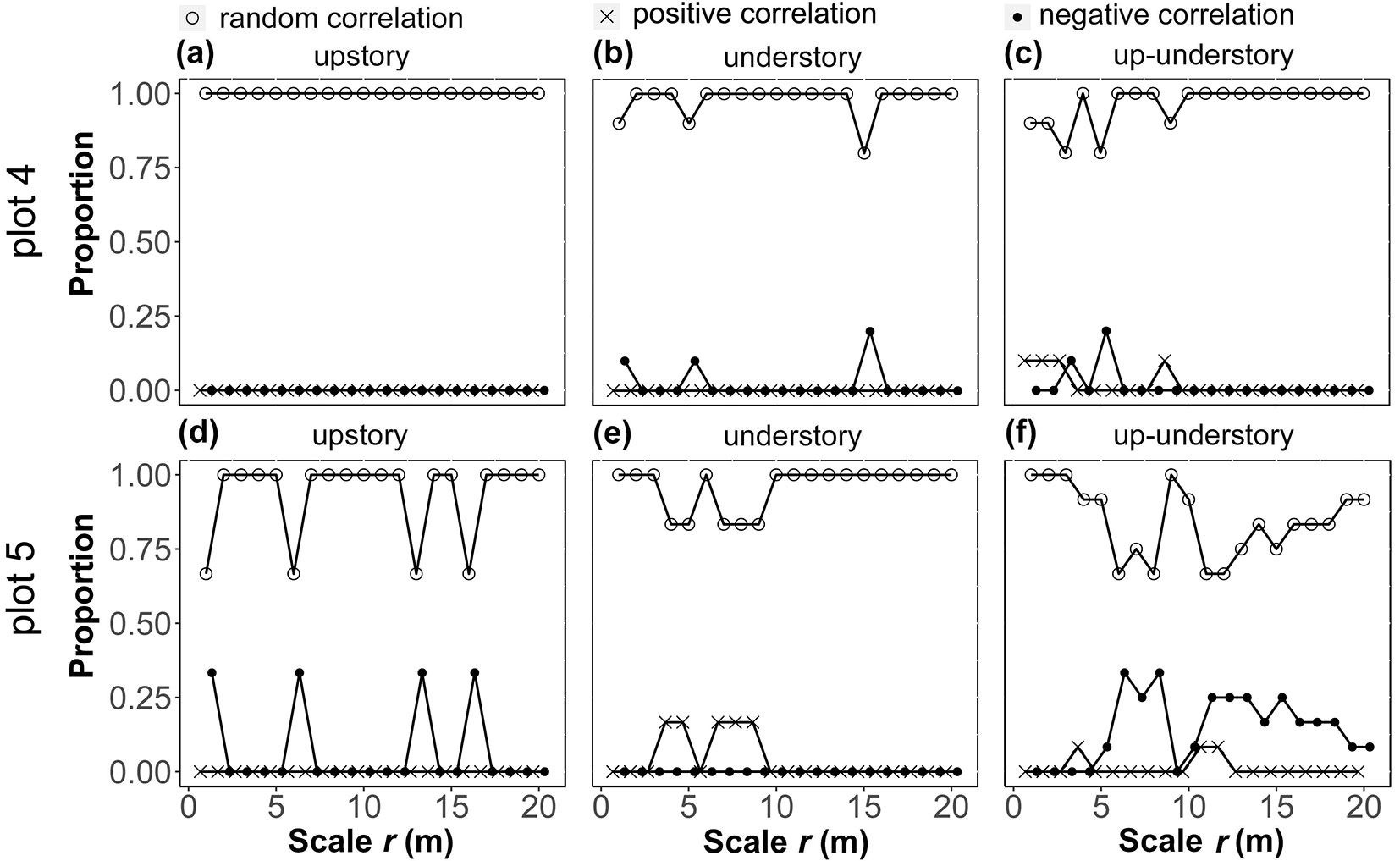
The populations of the main species of the upper layer of the two stands were mostly randomly correlated, and there were no positive correlations. The upper layer of plot 4 was all randomly correlated (Fig. 5a), but in plot 5 there was a weak negative correlation (17.0%) at some scales (r = 0-2, 5-7, 12-14, and 15-17 m - Fig. 5d). The features of the lower layer were similar to those of the upper layer. Plot 4 had a 10.0% negative correlation at r = 0-2 and 4-6 m, and a 20.0% negative correlation at r = 14-16 m, while there was a random correlation at the other scales (Fig. 5b). Plot 5 had a 16.7% positive correlation at r = 3-6 and 6-10 m, and a random correlation at the other scales (Fig. 5e). There was either a positive or negative correlation (10.0-20.0%) between the main populations of the upper and lower layers at small scales (r = 0-5 m) in plot 4, but almost all of them were random correlations at medium to large scales (r = 6-20 m - Fig. 5c). Although plot 5 was mostly random at small scales, there was a negative correlation (8.0-33.0%) between species at medium and large scales (Fig. 5f).

Fig. 5 - Statistical plots of the spatial correlation of the main tree species among the upstory and understory, and the relationship between the upstory and understory. After calculating the inter- and intra-specific spatial correlations in the different vertical layers by pairs, we considered the same type of spatial correlation (i.e., repulsion, attraction, and no relationship) at each scale divided by meters.

  Enlarge/Shrink   Download   Full Width  Open in Viewer

Spatial distributions of tree species

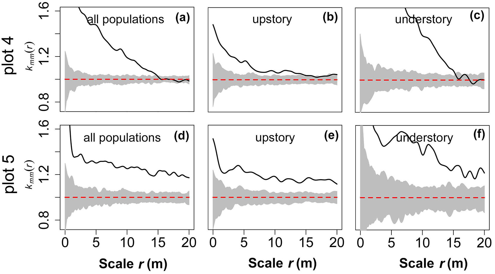
In plot 4, both the community and upper layer are a conspecies aggregation up to 15 m, but the aggregation of the community was much higher than that of the upper layer. At larger scales (r = 15-20 m), there was no obvious spatial correlation between or within species (Fig. 6a, Fig. 6b). In the lower layer, the same species were significantly concentrated at medium and small scales (r = 0-15.5 m), but the aggregation intensity weakened rapidly at larger scales (r = 15.5-20 m) until they became independent (Fig. 6c). The observed values of tree species in plot 5 deviated far from the 95% confidence limits of the MC simulation at all scales (r = 0-20 m), implying intensive conspecies aggregation or severe interspecific rejection in species (Fig. 6d-f).

Fig. 6 - Distribution pattern of species based on the null model of CSR. The grey background in each figure denotes the 95% confidence limits of a MC simulation. The black solid line represents the observed value and the red dashed lines are theoretical values.

  Enlarge/Shrink   Download   Full Width  Open in Viewer

Spatial distributions of tree sizes

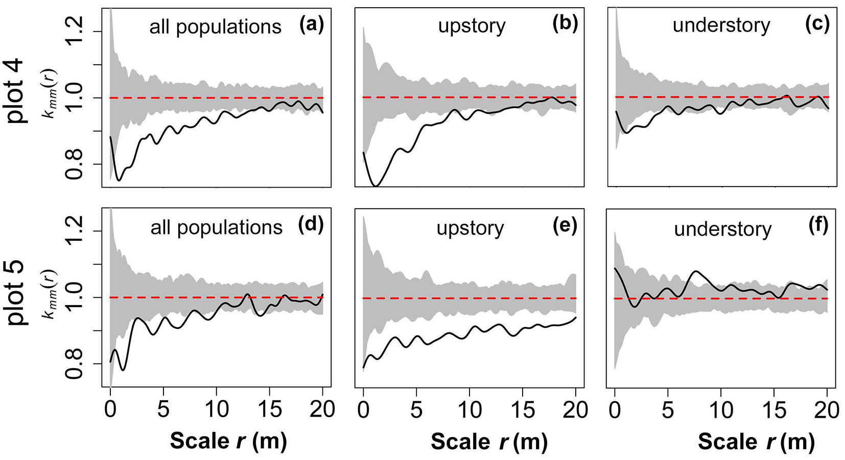
In plot 4, small trees were aggregated together at small to medium scales (r = 0-14 m), while trees with different DBH values were located independently of each other at the large scale (r = 14-20 m - Fig. 7a). The upper layer was similar, except that the trees with different DBH values were located independently of each other when r = 12 m (Fig. 7b). In contrast, the observed values in the lower layer were closer to the 95% confidence limits of the MC simulation at medium and small scales. Trees with different DBH values were located independently of each other at r = 0-1, 5-9.5, and 10.5-20 m, while there was a slight association at a few other observation scales (r = 1-5, 9.5-10.5 m - Fig. 7c). The size distribution in plot 5 was similar to that in plot 4. Different tree sizes were mutually exclusive at r = 0-10 and 14-15 m, while they were mutually independent at r = 10-14 and 15-20 m (Fig. 7d). However, in the upper layer, the small trees were surrounded by other small trees and the separation between small-sized and big-sized trees was significant (Fig. 7e). In the lower layer, trees with different DBH values were generally located independently of each other and only aggregated at a small range (r = 7.5-9.5 m), suggesting that large trees were likely to be surrounded by other large trees (Fig. 7f).

Fig. 7 - Spatial pattern of tree sizes based on the null model of CSR. The grey background in each figure denotes the 95% confidence limits of a MC simulation. The black solid line represents the observed value and the red dashed lines are theoretical values.

  Enlarge/Shrink   Download   Full Width  Open in Viewer

  Discussion 

Response of the distribution pattern to stratification

An aggregated distribution of species is a common pattern in nature, especially in the early stages of succession ([32], [19], [37]). The forests investigated in this study originated from land where a virgin P. yunnanensis forest was fully cut. Site conditions after clear cutting tend to be homogeneous and only light-dependent species (e.g., P. yunnanensis, Q. variabilis, C. glauca) were the first to renew and develop into forest canopy dominant species. They had reached physiological maturity and the natural dispersal distance of their seeds was very limited ([1], [19], [16]), resulting in the progeny to come together and the understory to be clustered. Several light-dependent shrubs (e.g., P. emblica, V. bracteatum, C. stellatum, and W. uvariifolia) appeared in the gap with the improvement of habitat conditions, and some of them also become mature. Their limited height and production of succulent fruit further limited the propagation distance of the seeds (Tab. S1 in Supplementary material), further strengthening the aggregation of the understory ([44], [35]). Habitat heterogeneity on a small scale could not be excluded by the current Poisson heterogeneity process model and it may affect species composition and distribution ([3], [35]). Moreover, seasonal drought in the study area may be another reason for some populations to gather together ([18]). In the same subtropical region, secondary forest in the Dinghu Mountains in Guangdong Province and the Yingzuijie Huitong National Forest Reserve in Hunan Province also had similar distribution patterns in the early stages of succession ([19], [40]). Species richness and diversity may also be related to the overall distribution pattern of the two forests ([19], [12]).

The distribution pattern of the upper forest layer at each scale was significantly closer to a random distribution than that of the lower layer (Fig. 4b, Fig. 4f vs Fig. 4c, Fig. 4g). This phenomenon is widespread in many forests in tropical, subtropical, and temperate regions ([17], [32], [19], [20], [25]). This may be the result of the greater competitive pressure between plants in upper layers than in lower ones ([29]). Inter-/intraspecific competition for habitat resources (e.g., light, water, and nutrition) leads to self-thinning ([11], [28]), destroying the pattern originally generated by the restrictive seed distribution and resulting in a tendency toward a non-aggregated distribution ([35], [16]). The spatial pattern among the different life histories of the same population also showed that individuals in the large diameter classes were closer to having a random distribution than those in the medium classes ([35]). Li et al. ([19]) also found that the degree of aggregation within the community decreased with an increase in the diameter classes.

Response of interspecific relationships to stratification

Pinus yunnanensis and Q. variabilis were the main species in the upstory, with both being light-dependent. The canopy width of P. yunnanensis was small, but much taller than that of Q. variabilis (Fig. 2a, Fig. 2b). However, Q. variabilis is a deciduous tree. The difference in growth and physiological characteristics between the two species effectively avoids direct competition, which may be an important reason for their random association. In contrast, if two populations compete for space in the canopy, they are expected to be negatively correlated ([27]). The spatial correlation between the upper and lower layers and their main populations was very weak (Fig. 4d, Fig. 4h; Fig. 5c, Fig. 5f). This was very similar to a reported relationship between the upper and lower layers of a secondary forest formed by cutting a Cunninghamia lanceolata plantation in the same period (year 1950). The lower layer was completely random at observation scales up to 0-17 m ([40]). As mentioned above, the upper and lower layer species differ in light dependence, which may determine the spatial association between large and small trees. Similar phenomena exist between some other natural forest populations (for example, the Quercus petraea and Fagus sylvatica mixed forest in Europe - [27]). The random correlation between the upper and lower layers at small scales implies that the lower layer will exist for a long time ([40]).

At all observation scales, the main populations in the understory in both forests were mostly randomly correlated, i.e., there was almost no competition or dependency (Fig. 5b, Fig. 5e). This may be related to the degree of intraspecific aggregation. Intraspecific aggregation implies a significant reduction in the probability of interspecific separation. In an old temperate forest, Zhang et al. ([44]) found that six congeneric maples with different diameters had random spatial correlations. In vegetation community succession, species interactions promote random spatial patterns. This has been confirmed by actual survey data ([43]) and software simulations ([15]). However, the random association of the understory found in this study may be a transient phenomenon, because many understory species only occur in the early stages of succession and are eventually replaced by more shade-tolerant species. Nonetheless, it is well-known that vertical stratification of forests helps to reduce competition and promote coexistence ([24]).

Response of species spatial distribution to stratification

Conspecies tend to aggregate in nature. This is generally considered to be the combined result of seed dispersion restrictions, habitat flittering, habitat heterogeneity and ecological preferences ([19], [37]). Our study showed that conspecies aggregation not only occurred at the community level; the vertical layers in the early stage of succession also had aggregation characteristics, and their intensity decreased with an increase in observation scale (Fig. 6a-f). This trend is consistent with the results of previous studies ([12], [30], [37]). Although the total number of trees in the upper and lower layers was similar, the degree of aggregation in the upper layer was less than that in the lower layer (Fig. 6b, Fig. 6e vs. Fig. 6c, Fig. 6f). Pommerening & Uria-Diez ([30]) also found that species segregation increased with an increase in tree diameter in stands that had suffered different degrees of disturbance and were located in different zones, i.e., the probability of another tree species surrounding the tree was greater for a large tree than for a small tree. Other studies have also shown that tree size (DBH/U, dominance) and the degree of species mixture are positively correlated in natural communities ([20], [21]) and their dominant populations ([37]). Some studies consider this phenomenon to be a negative density effect ([28], [37]). Other studies explain it in terms of niche complementarity. The number of large trees in a community is limited, and higher species richness promotes tree size differentiation. Differences in attributes of different species can result in the available growth space of a woodland being more effectively filled ([12], [30], [37]).

These effects may have existed simultaneously in the plots studied here, but the niche complementarity is more important. The uneven distribution pattern of the upper layer results in patchy light conditions in the forest, and light-dependent species become established in locations with less shade, forming an aggregated distribution ([33]). Some populations (e.g., V. bracteatum and C. stellatum) contain a number of dead small trees (Tab. S1 in Supplementary material), which provides opportunities for the arrival and survival of other species. This also results in the pattern of surviving dominant trees having a regular distribution, with more dissimilar adjacent trees ([33], [30], [36]). Other shade-tolerating clumped populations (e.g., A. quinquegona) and newly emerging tree species (e.g., T. ciliata, Diospyros kaki silvestris) do not display growth decay or death, and their appearance is more consistent with the habitat. Therefore, we believe that the ecological effects of forest communities are related to the specific populations and development stages.

Response of the spatial distribution of tree size to stratification

Asymmetric competition results in size differentiation and death of adjacent trees. Therefore, tree size is often used to assess the intensity of competition between adjacent trees and to predict changes in the community distribution pattern ([33], [31], [36]). In this study, the product of the paired diameters within the small range of the upper layer was far less than the expected value (Fig. 7b, Fig. 7e), indicating that individual sizes varied greatly and small trees clumped together. Smaller individuals may grow more slowly than larger trees, which may accelerate the differentiation of tree sizes ([7]). In contrast, a size difference between individuals in the lower layer was not obvious (Fig. 7c, Fig. 7f). This layer was composed of multiple shrubs and small tree species (Fig. 2a, Fig. 2 b), indicating that competition between adjacent trees was not strong. The differences in size differentiation of the upper and lower layers also indicated that the upper layer experienced a greater competitive pressure than the lower layer, which was consistent with the distribution pattern and the size differentiation process reported in an artificial forest. Size differentiation becomes more obvious as the succession time increases ([7]).

There was almost no difference in the size differentiation of the upper layers at small observation scales between both plots (Fig. 7b, Fig. 7e), but their understories differed from each other (Fig. 7c, Fig. 7f). The size differentiation was more obvious in the stand with a higher density (Tab. S1 in Supplementary material). It is likely that the average individual in the denser plot occupied more space and had a relatively strong demand for environmental resources. Competition will lead to size differentiation ([20]). This is consistent with conspecies having more clumped distribution (Fig. 6c). In monoculture plantations, it is generally believed that competition facilitates the differentiation of tree size in crowded communities ([7], [38]). However, in a natural forest with multiple tree species, the interaction between adjacent trees is far more complicated than in artificial plantations ([31]). In addition to density factors, forest regeneration and the death of crushed trees are also factors related to size differentiation ([37]). Differences in the tolerance of adversity, life-history and functional traits between species may also be important for the differences in size differentiation between two forests. This was considered as a possibility given that the tree species composition of the lower layer in the two plots was not identical (Fig. 2a, Fig. 2b).

  List of abbreviations 

The following abbreviations have been used throughout the manuscript:

1. MCF: mark correlation function
2. DBH: diameter at breast height
3. PCF: pair correction function
4. HP: habitat heterogeneity
5. CSR: complete spatial randomness
6. MC: Monte Carlo

  Acknowledgements 

This study was supported by the national natural science foundation of China (314 00542) and the Guangxi natural science foundation (2016GXNSFBA380233). Students from college of forestry, Guangxi University (Wenyan Tang, Xianyu Yao, Ting Pan, Jiafeng Long, Junmo Xu, Haihui Lu, Yao Li and Zhongfei Liu) participated in the wild investigation. We are very grateful for the comprehensive field service provided by the Guangxi Yachang national orchid natural reserve.

  References

  Supplementary Material

Fig. S1 - The location of our study sites, Yachang Township, Leye County, Baise City, Guangxi Zhuang Autonomous Region.
Fig. S2 - The secondary pine-oak forests subjected to clear-cutting 57 years ago currently displays two layers: the understory species mainly consists of evergreen broad-leaved shrubs, while the upstory mainly contains several deciduous broad-leaved species and P. yunnanensis.
Tab S1 - The parameters of main populations occurred in our sampled plots (the number of living trees ≥ 40) and their ecological characteristics.