Seeing trees from space: above-ground biomass estimates of intact and degraded montane rainforests from high-resolution optical imagery
iForest - Biogeosciences and Forestry, Volume 10, Issue 3, Pages 625-634 (2017)
doi: https://doi.org/10.3832/ifor2204-010
Published: Jun 01, 2017 - Copyright © 2017 SISEF
Research Articles
Abstract
Accurately quantifying the above-ground carbon stock of tropical rainforest trees is the core component of “Reduction of Emissions from Deforestation and Forest Degradation-plus” (REDD+) projects and is important for evaluating the effects of anthropogenic global change. We used high-resolution optical imagery (IKONOS-2) to identify individual tree crowns in intact and degraded rainforests in the mountains of Northern Borneo, comparing our results with 50 ground-based plots dispersed in intact and degraded forests, within which all stems > 10 cm in diameter were measured and identified to species or genus. We used the dimensions of tree crowns detected in the imagery to estimate above-ground biomasses (AGBs) of individual trees and plots. To this purpose, preprocessed IKONOS imagery was segmented using a watershed algorithm; stem diameter values were then estimated from the cross-sectional crown areas of these trees using regression relationships obtained from ground-based measurements. Finally, we calculated the biomass of each tree (AGBT, in kg), and the AGB of plots by summation (AGBP, in Mg ha-1). Remotely sensed estimates of mean AGBT were similar to ground-based estimates in intact and degraded forests, even though small trees could not be detected from space-borne sensors. The intact and degraded forests not only had different AGB but were also dissimilar in biodiversity. A tree-centric approach to carbon mapping based on high-resolution optical imagery, could be a cheap alternative to airborne laser-scanning.
Keywords
Biomass Estimation, Crown Area, IKONOS-2, Tree Community Similarity, Sabah
Introduction
Tropical rainforests are important sinks and sources in global carbon cycling. Annually, 15 to 25% of global greenhouse gas emissions are produced by loss of tropical rainforests, while increases in carbon within old-growth forests may offset 17% of emissions ([33]). While fossil fuel emissions increased by 29% between 2000 and 2008, emissions from land-use changes were nearly constant ([29]). These accelerated emissions, especially carbon-based emissions, are the causes of global warming, which affects forest ecosystems worldwide. Deforestation contributes to carbon emissions from land use changes in forests ([11]), whereas forest degradation is a direct human-induced activity that leads to a long-term reduction in forest carbon stocks ([26]). In Borneo, most lowland primary forest has been lost as a result of deforestation and forest degradation over the past 40 years ([28], [20]). The remaining uplands rainforests are severely threatened by increasing anthropogenic activities, particularly in the uplands of the Malaysian Borneon near Indonesia, where rates of loss are ten-times greater than across the border ([10]).
Accurate carbon stock estimates are essential for “Reduction of Emissions from Deforestation and Forest Degradation-plus” (REDD+) projects, which aims to pay governments for reductions in carbon dioxide emissions resulting from forest protection. REDD+ is regarded as a cost-effective mechanism for reducing global greenhouse gas emissions ([46]), but will only function effectively if carbon savings from avoided deforestation can be calculated cheaply and reliably at high resolution ([5]). In the context of REDD+, forest above-ground biomass (AGBp, in Mg ha-1) is best estimated from field-based inventory datasets: stem diameter of trees within plots are measured by hand and individual tree biomass calculated from published allometric formulae, which when summed and multiplied by carbon content gives above-ground carbon density ([11]). Whilst inventory plots will continue to contribute significantly to regional-scale carbon assessments, a dearth of plots in tropical regions and the expense of establishing new networks mean that analysts are increasingly looking to remote-sensing technology to measure forest stocks and changes ([11]).
The ability of capturing vegetation height information allows airborne LiDAR to outperform optical satellite imageries in accurately mapping forest AGB, but it is expensive for large area application. On the other hand, recent studies demonstrate that high-resolution satellite imageries can be used to examine forest canopy structure ([51], [41]). Information about individual tree crown (ITC) can be extracted by recognizing individual treetops ([50], [51]) and crown ([30], [51], [22], [40]). Treetop locations are usually extracted from high resolution imagery using local maximum filtering, an approach that is most accurate for low density woodlands where tree spacing is less than one individual per 6.6 m2 ([38]). Tree crowns are commonly delineated from high-resolution satellite imagery using either the watershed method ([41], [22], [40]) or valley-following method ([30], [21]), both of which are founded on reflectance being highest at the top of a crown and decreasing towards its edges ([16]). Tree biomasses can be calculated from these crown area estimates. Several studies have found significant relations between imagery-estimated crown area and field-measured diameter at breast height (DBH - [31], [37], [22], [40]), while foresters have published many papers relating DBH to above-ground biomass ([52], [7], [9], [8], [13]). Thus, in principle at least, carbon density can be estimated from high-resolution satellite imagery using an approach analogous to traditional field inventory methods. However, ITC segmentation is not always very accurate, and small trees are invisible on an optical remote sensing imagery, so biases and imprecisions in carbon estimates can arise. Few studies have critically evaluated the performance of this approach for estimating tropical carbon.
Most of these remote sensing studies emphasized carbon stock estimation for REDD+, though ensuring the protection of livelihoods and biodiversity is also central to the mechanism ([19], [35]). There may be risks to biodiversity that arise directly or indirectly from the activities under REDD+ ([49]), which needs to be monitored as co-benefits of REDD+ programmes. Monitoring tree species richness of disturbed tropical forests is complex because of high spatial heterogeneity ([43]), and comparisons of community similarity has thus been proposed as a robust and cost effective biodiversity index for REDD+ ([23], [24]).
This study aimed to estimate the carbon density of tropical montane rainforests from the IKONOS-2 imagery, by considering forest degradation, and examining the relationship between the estimated AGBp and biodiversity to ecologically validate the AGBp estimation. We examined the correlations between crown dimension estimates extracted from the IKONOS-2 imagery (satellite-based variables) and field-derived variables for intact and degraded forest types. Here, intact forest refers to relatively intact versus degraded along a spectrum from heavily logged to reduced-impact logging and old growth forests. We tested whether the dissimilarity in community composition was closely related to dissimilarity in forest biomass within these ecosystems, as would be anticipated from succession theory; if such a link could be found then mapping AGB would also allow one important aspect of forest biodiversity (namely dissimilarity to intact forest) to be mapped. Finally, a tree-level AGB (AGBT) distribution map was produced for the study area.
Materials and methods
Study area
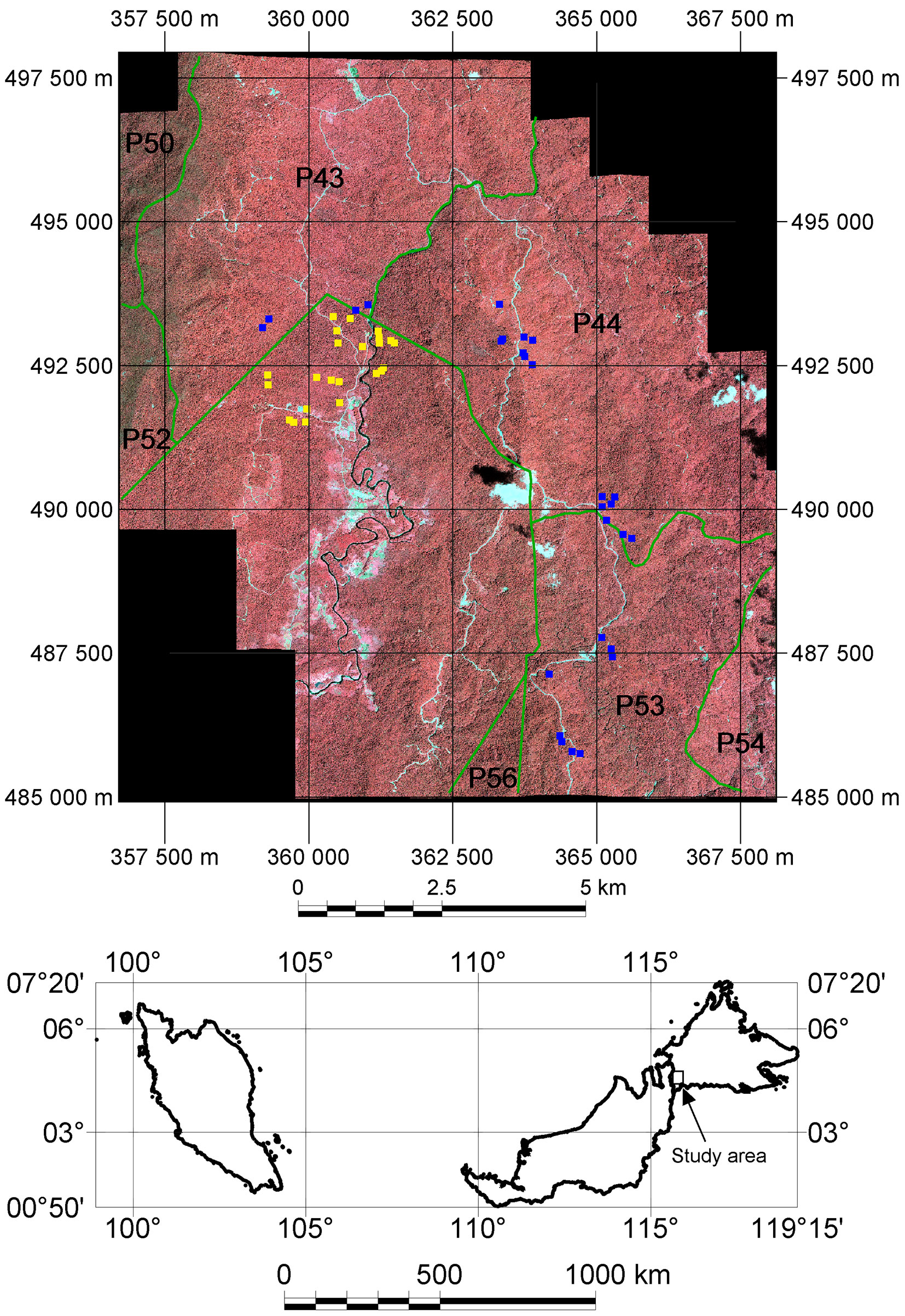
The study area is part of Ulu Padas area in the northern part of Borneo, near the international border between Sabah, Malaysia and Kalimantan, Indonesia (Fig. 1). Approximately 70% of the Ulu Padas area is lower montane oak-chestnut forest, which is distributed at elevations between 1150 and 1500 m a.s.l. The terrain of the study area is undulating to hilly, with steep slopes especially at the western part of the study area. Of the over 1500 specimens collected in our study area, more than one-quarter of the species correspond to the typical montane forest families of Fagaceae, Lauraceae and Guttiferae. Only seven species were from Dipterocarpaceae.
Fig. 1 - The IKONOS-2 imagery of the study area. Green line indicates compartment boundary of the Sabah Forest Industries (SFI). Polygon incuding yellow points (field plots) is land belonging to the state. Blue points are field plots collected at compartments P43, P44 and P53 within SFI concession area.
Almost half of the study area is owned by the Sabah state government, with local people (in Long Mio and Long Pasia villages) having a customary right to support their livelihoods from this land, and practicing slash-and-burn cultivation in it. Much of this state-land was selectively logged in the 1980s and early 1990s by commercial companies (personal communication, Head of Long Mio village, July, 2012). The other half of our study area is a concession managed by Sabah Forest Industries Sdn. Bhd. (SFI), which was established in 1983 as a government-owned company to produce pulp and paper, then privatized in 1993. SFI manages 288.623 ha of land, of which 183.346 ha are zoned as integrated timber plantations intended for the production of materials for pulp and paper. Currently about 46.000 ha of the zone is planted with Acacia and Eucalyptus species, while 104.822 ha are managed under so-called natural forest management (NFM). The harvest records of SFI indicate that the study area consists of an NFM area that was logged between 1997 and 2002. Since the turn of the millennium, the Sabah Forestry Department has required that NFM areas are managed using reduced impact logging methods; given the timing of the logging, it is unclear whether reduced impact logging was employed.
Field data collection
Field data were collected between November 2011 and October 2012. A total of 50 square plots of 30 × 30 m were established in random locations. In 48 of these plots, all trees with a DBH > 10 cm were characterized by measuring their DBH, height and tree position. The remaining two plots consisted mostly of small trees, so all stems with DBH > 5 cm were measured. The plot coordinates were determined by post-processing of differential GPS data (Ashtech ProMark 100®, Spectra Precision, Westminster, CO, USA). Tree height was measured using TruPulse laser range finder. The tree positions were measured in XY distance using TruPulse or distometer relative to the plot’s boundary. Of the 50 plots, 27 were located within the NFM areas, and the remainder in the state land. In total, 3709 trees were measured in these plots.
The forests were classified into two categories - intact and degraded forests - based on field assessment of forest condition, floristic composition and land use activities. The land use history was obtained from interviews with local villagers and forest management data of the SFI. Reduced impact logging areas and village reserve forest were categorized as intact, whereas slash-and-burn cultivation and conventional logging areas were categorized as degraded. Whilst forests subjected to reduced-impact logging are likely to exhibit lower biomass than old-growth forest, their recovery can be remarkably rapid ([43]) and the species composition is much more similar to old-growth forest than that of conventionally logged forest ([23]); for this reason we include them in the intact forest category. In addition, patches with AGB exceeding 200 Mg ha-1 were classified as intact forest; this threshold is widely used to differentiate intact and degraded tropical forests ([3], [34]).
We used allometric equations developed specifically for Bornean rainforest trees ([52], [8], [27]). The AGB (kg) of trees in intact forests was calculated from DBH (cm) as follows (eqn. 1):
using a regression relationship obtained for lowland rainforest by Yamakura et al. ([52]). This equation gives biomasses approximately 25% above those obtained by the wood-density corrected allometric model of Chave et al. ([13]) based on a global dataset. In degraded forests the following relationship, developed for this type of forest ([27]), was used (eqn. 2):
Biomass predictions from this formula are approximately half that given by the intact forest equation, because the early successional species found in these sites have much lower wood density (~0.35 compared to 0.36-0.81 - [53]).
Atmospheric and topographic correction of satellite imagery
An IKONOS-2 imagery acquired on 28 February 2010 was used in this study. Ortho-rectification was conducted using the rational polynomial coefficients file and the 30-m resolution Digital Elevation Model of the Shuttle Radar Topography Mission (SRTM-DEM) without ground control point (GCP). The ortho-rectification was assessed by calculating Root Mean Square (RMS) Residual from GCPs when compared to a Digital Surface Model generated from airborne LiDAR data. The RMS Residual was 1.13 m. IKONOS-2 has four multi-spectral bands of 4-m resolution. The panchromatic band of IKONOS-2 has a spatial resolution of 1 m. The spectral radiance of the multi-spectral and panchromatic bands was calculated using the published calibration values.
Atmospheric correction aims at removing the scattering and absorption ([48]). The scattering effect - mainly due to path radiance - was corrected using the dark object subtraction method ([14]); the dark object value for each band was determined by examining the lower end of each histogram: the influence of haze is indicated by a sharp increase in the number of pixels at nonzero radiance ([14]).
In the hilly study area, the brightness values of pixels vary as a result of differences in shading. These effects were reduced by topographic normalization of the IKONOS-2 imagery, using a non-Lambertian method with a Minnaert constant ([44]). We resampled the SRTM digital elevation model to the IKONOS-2 imagery’s resolution to derive the slope and aspect for the correction. The Minnaert coefficient k describes the surface’s bi-directional reflectance distribution function, where the scattering depends on the surface roughness ([44]). The value of k varies between 0 and 1, with 1 representing a perfectly diffuse reflector and a small value representing anisotropic scattering specific to the scene. The pixels of the intact forest were sampled to determine the values of k using linear regression analysis, and a backward radiance correction carried out ([44]).
Tree crown delineation
The geo- and atmospherically corrected IKONOS imagery were further processed before applying a tree-top recognition algorithm. First, we used principal component pan-sharpening to combine the four multispectral bands of 4-m resolution with the 1-m panchromatic band. A mask was then generated to filter non-vegetated areas (bare land, clouds and cloud shadows) from the vegetation we wished to segment. The mask was created by manually thresholding the normalized difference vegetation index (NDVI) from the IKONOS imagery to distinguish vegetation from non-vegetation areas, and removing shadows using the panchromatic band ([4]). Finally, inverse image of the pan-sharpened image was generated. The inverted pan-sharpened image was input into a watershed algorithm to delineate individual tree crowns ([22]). All these analyses were conducted in ArcGIS 9® (ESRI, Redwood, CA, USA). The polygons delineated using the watershed method were overlaid with the plot location to determine the crown polygons for each plot. The segmentation results were compared with the tree positions from the plot data to evaluate the crown delineation in each plot; polygons with centroid within a plot were considered as trees within that plot. Because lower canopy trees cannot be observed by the satellite sensor, we applied the general principle that considers tree crowns spotted in high-resolution satellite data are most likely to correspond with the largest trees observed in the plot ([37], [22]). Say that n trees are delineated from the imagery in a given plot; if the stems measured in the plot are ranked from largest to the smallest based on DBH, then the first n trees in the ranking are likely to correspond to the remotely sensed trees. Along with the ranked trees, we compared the tree position and measured crown size between a delineated crown and field measured crown. We discarded any delineated crown that was a sub-crown or included several crowns.
Crown delineation accuracy was assessed by comparing automatically and manually segmented imageries ([15]). A total of 1104 upper-canopy crowns within 35 plots were visually interpreted and digitized to assess the delineation accuracy. The simplest test of segmentation accuracy is to compare the number of “reference crowns” (i.e., those manually segmented) with the number of automatically segmented crowns. Secondly, the degree of spatial overlap between crowns can be determined. The degree to which automatically and manually delineated crown areas overlap was used to calculate the over-segmentation index (eqn. 3):
where OS is the oversegmentation index (poor = 1, excellent = 0), X = {xi: i=1, …, n} and Y = {yj: j=1, …, n}. X are the automatically delineated crowns and Y are the largest n reference crowns. For under-segmentation (US), it was calculated as follows (eqn. 4):
The overall quality of segmentation is then given by the closeness index (D - eqn. 5):
Lower values of D indicate better segmentation results.
Estimation of the above-ground biomass of trees and carbon density
Segmentation of the IKONOS-2 imagery generated three crown related variables: crown perimeter (CP_I) and crown area (CA_I), and the crown diameter calculated from the crown area using a circular shape formula (CD_I). Pearson’s correlation was used to test which of these variables was most closely related to field-derived AGB (or structural variables), and then this variable was used to create a statistical estimation model by least squares regression. Half the plots with delineated tree crown data were selected at random for model building, whilst the other half were kept for model validation. The estimated tree-AGB was compared with the observed tree-AGB from the field measurements.
Tree community composition
We initially identified species of all trees on the plots by local names. Plant specimens were then taken for identification at the herbarium of the Forest Research Center in Sandakan, Sabah. We used nonmetric multidimensional scaling (NMDS) to analyze the variation in tree community composition among plots ([23], [24]), which is a nonparametric method giving ecologically meaningful measures of community dissimilarity. The relative basal area of each species in 50 plots was used to calculate the dissimilarity among plots ([12]). Differences among tree communities were examined by looking at the first and second axes of variation from the ordination analysis; differences among forest types were analyzed by permutational multivariate analysis of variance (PERMANOVA - [2]), using the “adonis” function in the “vegan” package of R ([36]).
Results
Tree crown delineation
A total of 1584 upper-canopy tree crowns were detected within the 50 plots (Tab. 1), which is almost half of the total number of trees measured on the ground, suggesting that the majority of trees were hidden under the canopy. The closeness index (D) to the reference tree crowns was 0.36 (i.e., the accuracy of segmentation was 64%). Delineation rate varied between forest types: it was on average 49% accurate (range 28-93%) in intact forest, where trees were large and densities low, but only 39% accurate (range 16-78%) in degraded forest where there were many small trees and lianas. The upper-canopy trees we detected had mean DBH = 29.7 cm (± 1 standard error of mean of 14.9 cm) and mean height of 23.2 ± 7.6 m in intact forest. Detected trees were much smaller in the degraded forest, with a mean DBH of 20.9 ± 7.6 cm and mean height of 18.5 ± 5.1 m.
Tab. 1 - Characteristics of the delineated tree crowns for intact and degraded forests (50 plots).
| Forest Type | Characteristics | Minimum | Maximum | Mean | Std. Error | Std. Deviation |
|---|---|---|---|---|---|---|
| Intact forest (26 plots) |
Closeness index (%) | 0.28 | 0.93 | 0.49 | 0.25 | 0.17 |
| Field-derived DBH (cm) | 10.40 | 122.10 | 29.73 | 0.53 | 14.86 | |
| Field-derived Height (m) | 7.60 | 65.90 | 23.15 | 0.27 | 7.55 | |
| Tree density (n ha-1) | 300.00 | 1077.78 | 605.13 | 29.82 | 152.06 | |
| Degraded forest (24 plots) |
Closeness index | 0.16 | 0.78 | 0.39 | 0.31 | 0.15 |
| Field-derived DBH (cm) | 10.10 | 80.80 | 20.90 | 0.27 | 7.60 | |
| Field-derived Height (m) | 5.10 | 41.80 | 18.47 | 0.18 | 5.12 | |
| Tree density (n ha-1) | 355.56 | 3850.00 | 1220.72 | 158.72 | 775.30 |
Crown dimension estimates of the detected trees were compared to field-derived variables (Tab. 2). For the intact forest, most of the field-derived variables were significantly correlated with the satellite-based variables: DBH was highly correlated with remotely sensed crown dimension variables (CA_I: r = 0.87; CD_I: r = 0.86; CP_I: r = 0.84), but field-derived tree height (Ht_f) was more weakly correlated with satellite-based variables (r ranging from 0.53 to 0.57). Field-derived AGB was moderately correlated with CA_I (r = 0.73), CD_I (r = 0.69) and CP_I (r = 0.67). Similarly correlations were found for the degraded forest: DBH was highly correlated with the satellite-based variables CA_I (r = 0.81), CD_I (r = 0.79) and CP_I (r = 0.77), while tree height was less well correlated with them. Similarly, we only found moderate correlations between field-derived AGB and with the three satellite-based variables (r value 0.64-0.71).
Tab. 2 - Correlations between the satellite-based (I) and field-derived (f) estimates of individual tree characteristics for the intact and degraded forests. (CA_I): Satellite-based crown area; (CP_I): satellite-based crown perimeter; (CD_I): satellite-based crown diameter; (Ht_f): field-derived tree height; (DBH_f): field-derived stem diameter; (AGB_f): field-derived above ground biomass. (**): Correlation is significant at the 0.01 level (2-tailed).
| Forest Type | Estimates | CA_I | CP_I | CD_I | Ht_f | DBH_f | AGB_f |
|---|---|---|---|---|---|---|---|
| Intact forest (396 trees in 13 plots) |
CA_I | 1 | - | - | - | - | - |
| CP_I | 0.943** | 1 | - | - | - | - | |
| CD_I | 0.981** | 0.960** | 1 | - | - | - | |
| Ht_f | 0.547** | 0.531** | 0.572** | 1 | - | - | |
| DBH_f | 0.871** | 0.836** | 0.862** | 0.676** | 1 | - | |
| AGB_f | 0.734** | 0.669** | 0.685** | 0.548** | 0.915** | 1 | |
| Degraded forest (390 trees in 12 plots) |
CA_I | 1 | - | - | - | - | - |
| CP_I | 0.946** | 1 | - | - | - | - | |
| CD_I | 0.976** | 0.962** | 1 | - | - | - | |
| Ht_f | 0.509** | 0.501** | 0.514** | 1 | - | - | |
| DBH_f | 0.811** | 0.772** | 0.789** | 0.684** | 1 | - | |
| AGB_f | 0.711** | 0.639** | 0.639** | 0.486** | 0.879** | 1 |
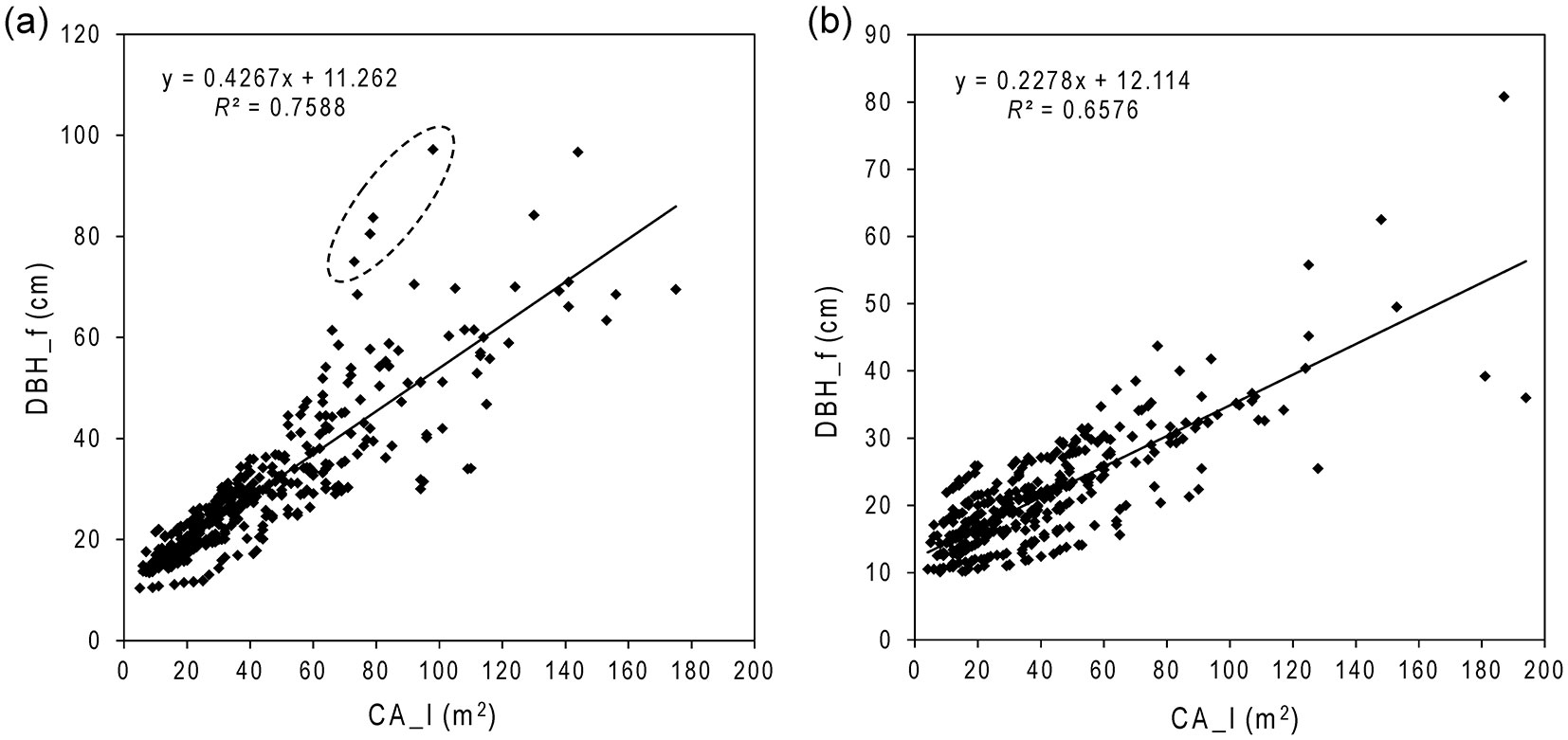
Fig. 2 - DBH estimation models using CA_I for the intact (a) and degraded (b) forests. Crown area was well correlated with DBH, especially below 50 cm. Considerable variations were observed for DBH > 60 cm. A few old trees with large DBH (in the dashed circle in panel a) have relatively small crown areas. This reflects the typical condition of an intact tropical rainforest.
Based on these correlation analyses, the best-performing satellite-based variable (CA_I) was used as the independent variable in regression models, which was then used to estimate DBH of all upper-canopy trees in the intact and degraded forests. With field measurements, we found that polynomial (R2= 0.68) and linear (R2= 0.67) regression functions only differed by 1%. Therefore, we used a straight line relationship to estimate DBH from CA_I (m2). DBH_f and CA_I exhibited a strong positive biophysical relationship (R2 = 0.76 and 0.66 in intact and degraded forests, respectively - Fig. 2). The regression models for estimating the DBH (cm) for the intact (DBHIF) and the degraded (DBHDF) forests were as follows (eqn. 6, eqn. 7):
For intact forest DBHIF = 11.3 + 0.427 · CA_I (R2 = 0.76; SEs of parameters 0.635 and 0.012, respectively), which was highly statistically significant (F[1, 393] = 1236, p < 0.0001). For degraded forest DBHDF = 12.1 + 0.228 · CA_I (R2 = 0.66; SEs of parameters 0.409 and 0.008, respectively), which was also highly statistically significant (F[1, 387] = 743, p < 0.0001).
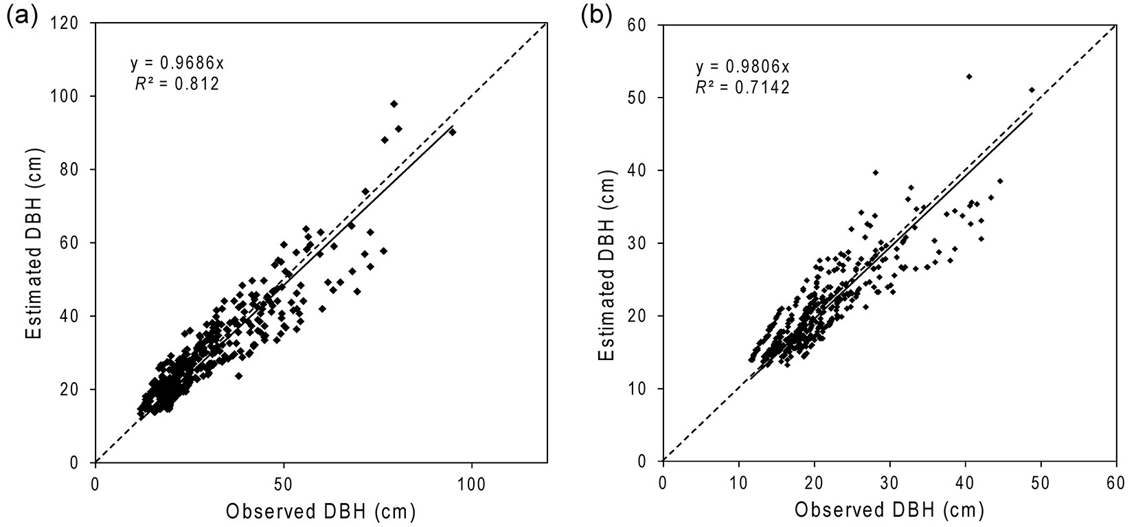
Plots of observed vs. estimated DBH for the intact and degraded forests with validation datasets (Fig. 3a, Fig. 3b) had slopes of 0.97 and 0.98, when forced through the origin, demonstrating that they were virtually unbiased. The mean of the observed DBH values was very similar to the mean of the estimated values (Tab. 3).
Fig. 3 - Observed vs. estimated DBH for the intact (a) and degraded (b) forests. Overall, DBH was very well estimated by the models for both forests. However, larger trees (DBH > 50 cm for intact and DBH > 35 cm for degraded forests) seemed to be under-estimated.
Tab. 3 - Validation of DBH and tree AGB estimation for intact and degraded forests (based on independent 25 plots of validation dataset).
| Forest Type | Parameter | Min | Max | Mean | Std. Error |
Std. Deviation |
|---|---|---|---|---|---|---|
| Intact forest (387 trees in 13 plots) |
CA_I (m2) | 5.00 | 203.00 | 43.34 | 1.54 | 30.32 |
| Observed DBH (cm) | 12.00 | 94.80 | 29.74 | 0.73 | 14.34 | |
| Estimated DBH (cm) | 13.40 | 97.88 | 29.78 | 0.66 | 12.94 | |
| Observed AGB (kg tree-1) | 67.39 | 15148.18 | 1125.51 | 86.96 | 1708.46 | |
| Estimated AGB (kg tree-1) | 89.90 | 16472.72 | 1058.00 | 86.30 | 1695.48 | |
| Degraded forest (410 trees in 12 plots) |
CA_I (m2) | 4.00 | 179.00 | 36.90 | 1.27 | 25.65 |
| Observed DBH (cm) | 11.60 | 48.80 | 20.55 | 0.33 | 6.55 | |
| Estimated DBH (cm) | 13.03 | 52.89 | 20.57 | 0.29 | 5.85 | |
| Observed AGB (kg tree-1) | 32.00 | 1050.55 | 152.01 | 7.03 | 142.01 | |
| Estimated AGB (kg tree-1) | 42.41 | 1277.49 | 147.34 | 6.31 | 127.39 |
Estimation of above-ground biomass of individual trees
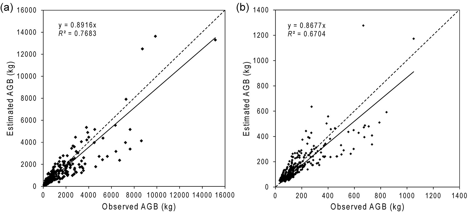
Tree AGBT calculated from estimated DBH values were very similar to the observed AGBT for the intact and the degraded forests (Tab. 3). For the intact forest, the estimated AGBT ranged between 90 kg and 16.473 kg, with a mean of 1.058 kg, which was approximately 6% lower than the observed AGBT for the intact forest. Both the minimum and maximum of the estimated AGBT for the degraded forest were much lower than the intact forest: only 42 kg and 1.277 kg. The mean estimated AGBT of the degraded forest was 147 kg, which was about 3% lower than the observed AGBT. Regressions of observed vs. fitted values (through the origin) had a slope of 0.89 and 0.87 for intact and degraded forests, respectively (Fig. 4).
Fig. 4 - Observed vs. estimated tree AGB for the intact (a) and degraded (b) forests. The under-estimation of DBH for larger trees had led to under-estimation of AGB for those trees.
AGBP values were calculated by summing the AGBT of all trees delineated per plot and converting to Mg per hectare. The field-derived AGBP for intact and degraded forests were under-estimated by about 10% and 20% (Tab. 4), which is greater than the under-estimation individual tree AGB. This additional biomass arises because smaller trees were not visible in the imagery, and although they individually have low AGBT they are numerous. RMSE of the estimates were 135 and 20 Mg ha-1 for intact and degraded forests, respectively, representing 34% and 30% of the average observed AGBP.
Tab. 4 - Root-mean-square error (RMSE) of the AGB estimation for intact and degraded forests (based on 25 independent plots in the validation dataset). Average estimation was calculated as percent of the estimated AGB to the observed total AGB.
| Parameter | Intact forest | Degraded forest |
|---|---|---|
| RMSE (Mg ha-1) | 134.7 | 20.3 |
| RMSE (%) | 33.9 | 30.4 |
| Average estimation (%) | -7.7 | -20.7 |
Biodiversity similarity between intact and degraded forests
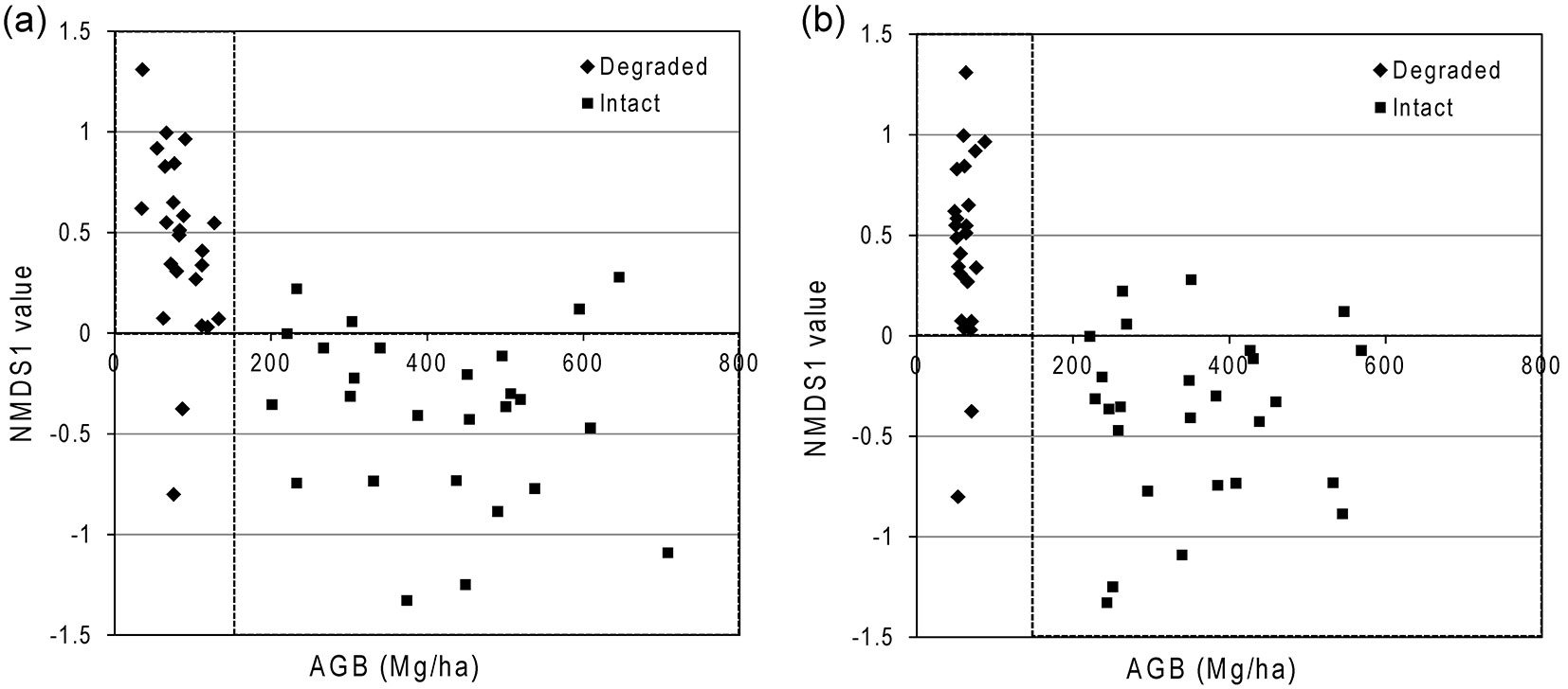
The first axis of the biodiversity ordination accounted for 53% of the total variation, reflecting a major proportion of dissimilarity among communities. There is a significant relationship between ground-based estimates of AGBP (i.e., an indicator of forest degradation) and NMDS axis 1 scores (Fig. 5a). Similar patterns were observed when plotting the imagery-estimated AGBP against the NMDS axis 1 scores (Fig. 5b). Intact and degraded forests are clearly differentiated by NMDS: almost all (92%) of the degraded forest plots had a positive axis-1 score, whilst most (85%) of the intact forest plots had a negative score on the NDMS axis 1.
The above-ground biomass distribution maps
Object-based classification approach with the nearest-neighbour classifier was used in eCognition software (Trimble) to classify the segmented IKONOS-2 imagery into intact and degraded forests using field observations of the forest structure, species composition and land use history to train the classifier. The NMDS results (Fig. 5a) were used to calculate overall accuracy and kappa statistic. Comparing these classifications with the field plot data, the overall accuracy and kappa statistic of the forest type classification were 82.0% and 0.64, respectively. The producer’s and user’s accuracies for the intact and degraded forests ranged between 75% and 88%. The forest type classification from the IKONOS-2 imagery indicated that the study area had 7036 ha of intact forest. Degraded forest covered about half the area of intact forest (3542 ha).
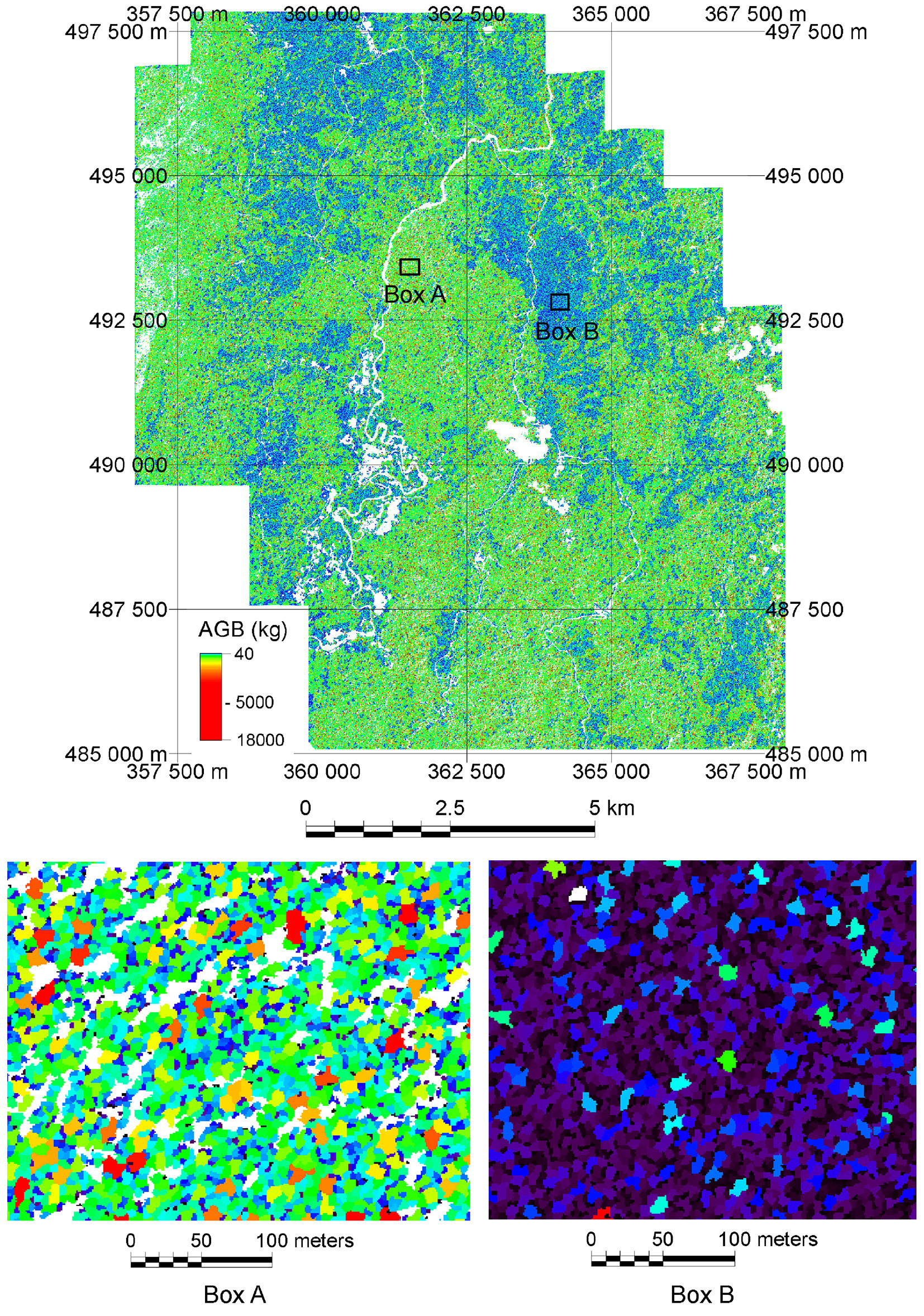
Fig. 6 shows the AGB distribution of the montane forests at the Ulu Padas area at tree level. To produce the AGBT map, eqn. 6 and eqn. 7 were used to estimate DBH for the intact and degraded forest trees in the segmented imageries, and then AGBT was calculated using the appropriate biomass allometries, i.e., eqn. 1 ([52]) and eqn. 2 ([27]) for intact forest and degraded forests, respectively. The map shows a strong influence of land-use activity on the spatial distribution of AGBT (Fig. 6). Most of the trees in the intact forest possess a large crown and thus have a high AGBT (more green and yellow colored polygons in Box A of Fig. 6). In contrast, most of the trees in the degraded forest were of a dark shade of blue color, indicating a lower AGBT (Box B in Fig. 6). The high AGBT in the intact forest was mainly found at forests subject to reduced impact logging operation, whereas the low AGBT in degraded forest in the stateland was mainly due to shifting cultivation activities.
Fig. 6 - Above-ground biomass (AGBT) map of the study area. AGBT of trees (kg) were assessed through DBH estimation by forest type. Boxes A and B are magnified areas of AGBT for the intact and degraded forests. Box A shows a typical area logged with reduced impact logging method, whereas Box B shows an example of regenerated forest at a shifting cultivation area.
Discussion
Tree centric approaches to biomass mapping
Optical imagery collected by satellites has long been regarded as unsatisfactory for the purposes of estimating the biomass or degradation status of tropical rain forest, because indices such as NDVI, based on the spectral characteristics of pixels, are known to saturate at high biomass ([39], [32], [28]). Here we show that recognizing individual trees from high-resolution optical imagery can overcome these problems. Crown area has proven to be a robust and sensitive variable for estimating DBH - and thence biomass - because of the linear relationship between crown area and DBH in both intact and degraded forests ([40]).
Overall, DBH estimation models for intact and degraded montane rainforests in northern Borneo were successful. The estimated AGBP has a mean of 647 Mg ha-1 and 176 Mg ha-1 for the intact and degraded forests, respectively. The small differences between the means of the estimated and observed AGBP for both forest types provided a convincing argument that the results of the satellite-based approach were consistent, overall. The scatter-plots between the estimated and observed values of AGB at tree level (Fig. 4) and plot level (Fig. 5) for both forest types confirmed the consistency of the estimation models. The RMSE for intact and degraded forests were 34% and 30% of the average observed AGBP, respectively. We also examined factors that affect the RMSE by analyzing the squared residual of the estimates against tree density per hectare and total AGB. Three outlier plots (Fig. 5), representing 12% of the validation plots, with high squared residuals were low in tree density but very high in total AGBP. This was due to the presence of few old, big trees (DBH > 80 cm) with relatively small crowns. Nevertheless, the slopes of the regression lines through the origins for the scatter-plots in Fig. 4 (degraded: y = 0.87 · x; intact: y = 0.89 · x) indicated that DBH estimation by considering forest degradation had a better fit compared with the combined forest types (y = 0.74 · x - [40]). Moreover, the two forest types were clearly different in terms of the statistics of DBH as well as AGB (Tab. 3).
Because of the extraordinary accuracy of airborne LiDAR in measuring canopy height, laser scanning is the best current technology for estimating the carbon density of tropical forests. Asner & Mascaro ([6]) have shown that simple regression relationships based on LiDAR estimates of mean canopy height can provide highly accurate carbon maps (R2 > 0.8), and can be applied to different regions of the world once adjusted for variation in wood density and forest packing. Airborne LiDAR surveys outperform spaceborne optical surveys: in Malaysian montane forests the RMSE of AGB estimates made by LiDAR was 26% of average AGB ([25]), which is about 8% and 4% lower than the results presented here for degraded and intact forests. However, provided that space-borne sensors can deliver unbiased estimates of AGB, they could be valuable at regional scales, even if any given pixel is measured at lower precision than possible from an aircraft. This is appealing, given the high cost of LiDAR data acquisition. In addition, a new generation of small satellites with optical sensors are being launched that will collect data much more frequently than the current earth observation satellites and should thereby overcome many of the problems associated with persistent cloud cover in the tropics.
Recently, Dalponte & Coomes ([17]) suggested that a tree-centric approach based on LiDAR imagery, based on fundamental principles of forest mensuration, can deliver results with a similar precision to the top-canopy-height method. Airborne LiDAR delivers more precise results because it measures both canopy height and canopy area, whereas the optical imagery only delivers canopy area information, and also because the 3D point cloud contains much richer structural information than the optical sensors. Future research could focus productively on using tree-centric airborne LiDAR approaches to better calibrate the spaceborne optical sensor approach described in this paper. The relationships between satellite-based crown variables and tree structural variables in a tropical forest also require further investigation. DBH is known to have a strong relationship with crown area ([7]) and crown diameter ([45]) in temperate forests, and a significant relationship has been found for an intact forest in Brazil ([37]), and in a montane forest in Malaysia ([40]). However, a comprehensive analysis has yet to be published.
Biodiversity mapping in the context of REDD+
We have shown that optical imagery can differentiate between intact and degraded montane rainforests. This is important in the context of REDD+. Linking biodiversity monitoring to carbon stock estimation is vital for effective implementation of REDD+, but even more critical is what aspect of biodiversity needs to be monitored ([18]). Tree community composition is consistent in describing biodiversity patterns ([47], [23]) and robust in indicating the response of tree assemblage to forest degradation due to anthropogenic disturbances ([23], [24]). Measuring tree community composition is cost effective for REDD+, because only upper canopy trees are to be measured, making it cheaper than biodiversity metrics based on wildlife monitoring ([24]). Our results demonstrated that the relationship between AGB and NMDS axis 1 based on field data (Fig. 5a) can be successfully reconstructed with the estimated AGB from satellite imagery (Fig. 5b). The intact and degraded forests were clearly separable at a value lower than the widely used AGB threshold of 200 Mg ha-1 ([3], [34]). The difference could be due to the fact that the AGB of a montane rainforest is usually lower than that of a lowland rainforest ([1]). Further in-depth study is needed to examine the application of this tree-centric approach as well as the AGB thresholds of forest degradation for different natural forest types using high-resolution satellite remote sensing. More generally, there is currently great interest in using remote sensing products to help monitor biodiversity ([42]). Incorporating remotely sensed maps of forest disturbance into biodiversity modelling efforts is likely to increase predictive power considerably.
Conclusions
Tropical forest biomass estimation using high-resolution satellite imageries has been receiving increasing attention, but its application to montane rainforests has not been adequately dealt with. Our results indicate that the use of high-resolution satellite imagery is useful in developing DBH estimation models, which can be used to estimate the AGB for intact and degraded montane rainforests in Northern Borneo. The crown area from the IKONOS-2 imagery was useful in estimating DBH for the intact and degraded forests, from which biomass can be estimated using published allometric equations.
Biodiversity safeguarding has been an important issue in REDD+ implementation in the tropics. The observed relationship between AGBP and the NMDS axis 1, an index of tree community dissimilarity, showed that intact and degraded forests were well differentiated, allowing to use our AGBP maps to map degradation. Tropical biodiversity should be examined in parallel with AGB estimation using satellite remote sensing, because this kind of inferential information is useful in guiding REDD+ activities that are related to conservation of forest carbon stocks, sustainable management of forests and enhancement of forest carbon stocks.
Acknowledgements
This project was funded by Ministry of Agriculture, Forestry and Fisheries Research Council, Government of Japan. Ministry of Higher Education, Government of Malaysia provided “Geran Sanjungan Penyelidikan” that motivates us for strengthening our international collaborations. We sincerely thank the Sabah Forestry Department (SFD) for research permission, the Sabah Forest Industry (SFI) for field support, and the Government of United States of America for some technical assistance.
References
CrossRef | Gscholar
CrossRef | Gscholar
CrossRef | Gscholar
Gscholar
CrossRef | Gscholar
CrossRef | Gscholar
CrossRef | Gscholar
CrossRef | Gscholar
Authors’ Info
Authors’ Affiliation
Zia-Yiing Ling
Wilson Wong
Alexius Korom
Keiko Ioki
Faculty of Science and Natural Resources, University of Malaysia Sabah, Jalan UMS, 88400 Kota Kinabalu, Sabah (Malaysia)
Department of Plant Sciences, University of Cambridge, Cambridge, CB2 3EA (UK)
Graduate School of Agricultural and Life Sciences, The University of Tokyo, 1-1-1 Yayoi, Bunkyo-ku, Tokyo 113-8567 (Japan)
Hideki Saito
Gen Takao
Forest and Forest Products Research Institute, Matsunosato 1, Tsukuba, Ibaraki 305-8687 (Japan)
Corresponding author
Paper Info
Citation
Phua M-H, Ling Z-Y, Coomes DA, Wong W, Korom A, Tsuyuki S, Ioki K, Hirata Y, Saito H, Takao G (2017). Seeing trees from space: above-ground biomass estimates of intact and degraded montane rainforests from high-resolution optical imagery. iForest 10: 625-634. - doi: 10.3832/ifor2204-010
Academic Editor
Davide Travaglini
Paper history
Received: Aug 22, 2016
Accepted: May 04, 2017
First online: Jun 01, 2017
Publication Date: Jun 30, 2017
Publication Time: 0.93 months
Copyright Information
© SISEF - The Italian Society of Silviculture and Forest Ecology 2017
Open Access
This article is distributed under the terms of the Creative Commons Attribution-Non Commercial 4.0 International (https://creativecommons.org/licenses/by-nc/4.0/), which permits unrestricted use, distribution, and reproduction in any medium, provided you give appropriate credit to the original author(s) and the source, provide a link to the Creative Commons license, and indicate if changes were made.
Web Metrics
Breakdown by View Type
Article Usage
Total Article Views: 48919
(from publication date up to now)
Breakdown by View Type
HTML Page Views: 40198
Abstract Page Views: 3338
PDF Downloads: 4121
Citation/Reference Downloads: 42
XML Downloads: 1220
Web Metrics
Days since publication: 3232
Overall contacts: 48919
Avg. contacts per week: 105.95
Article Citations
Article citations are based on data periodically collected from the Clarivate Web of Science web site
(last update: Mar 2025)
Total number of cites (since 2017): 6
Average cites per year: 0.67
Publication Metrics
by Dimensions ©
Articles citing this article
List of the papers citing this article based on CrossRef Cited-by.
Related Contents
iForest Similar Articles
Review Papers
Accuracy of determining specific parameters of the urban forest using remote sensing
vol. 12, pp. 498-510 (online: 02 December 2019)
Review Papers
Remote sensing-supported vegetation parameters for regional climate models: a brief review
vol. 3, pp. 98-101 (online: 15 July 2010)
Technical Reports
Detecting tree water deficit by very low altitude remote sensing
vol. 10, pp. 215-219 (online: 11 February 2017)
Research Articles
High resolution biomass mapping in tropical forests with LiDAR-derived Digital Models: Poás Volcano National Park (Costa Rica)
vol. 10, pp. 259-266 (online: 23 February 2017)
Review Papers
Remote sensing of selective logging in tropical forests: current state and future directions
vol. 13, pp. 286-300 (online: 10 July 2020)
Research Articles
Estimation of aboveground forest biomass in Galicia (NW Spain) by the combined use of LiDAR, LANDSAT ETM+ and National Forest Inventory data
vol. 10, pp. 590-596 (online: 15 May 2017)
Research Articles
Above ground biomass estimation from UAV high resolution RGB images and LiDAR data in a pine forest in Southern Italy
vol. 15, pp. 451-457 (online: 03 November 2022)
Research Articles
Geostatistical techniques for estimating aboveground biomass in eastern Amazonia
vol. 19, pp. 85-93 (online: 13 March 2026)
Research Articles
Assessing water quality by remote sensing in small lakes: the case study of Monticchio lakes in southern Italy
vol. 2, pp. 154-161 (online: 30 July 2009)
Research Articles
Evaluation of hydrological and erosive effects at the basin scale in relation to the severity of forest fires
vol. 12, pp. 427-434 (online: 01 September 2019)
iForest Database Search
Search By Author
Search By Keyword
Google Scholar Search
Citing Articles
Search By Author
Search By Keywords
PubMed Search
Search By Author
Search By Keyword

