Hot spot maps of forest presence in the Mediterranean basin
iForest - Biogeosciences and Forestry, Volume 9, Issue 5, Pages 766-774 (2016)
doi: https://doi.org/10.3832/ifor1802-009
Published: Jun 13, 2016 - Copyright © 2016 SISEF
Technical Reports
Abstract
The Mediterranean basin is one of the most varied areas worldwide in terms of biodiversity and species richness due to its climatic and geomorphological features, and it is characterized by multi-faceted habitats where forests play a crucial role. Nowadays, the geographic distribution of forest species is well known and multiple geographic datasets are available with different spatial details. However, protection and conservation strategies need more specific information to identify areas with high conservation priority or more vulnerable to the ongoing environmental change (“hot spots”). To this purpose, tree species distribution data were investigated through hot spot analysis using Geographic Information Systems. The analysis was carried out on presence data of ten relevant forest tree species/classes across Mediterranean Europe. By combining spatial analysis and spatial statistics, we identified high and very high hot spot areas for the selected species/classes, which were validated by assessing their biological significance. Given the sub-continental extent of the study, a multiple scale approach was applied ranging from regional, sub-regional to local scale, coherently with the potential multi-level and multi-sector users of similar data and tools. Our results confirm the feasibility of the approach used to increase the quality and quantity of information achievable from available forest distribution datasets. The hot spot maps obtained are a useful support for further spatial evaluations, and may help environmental decision makers to identify priority areas for forest protection and conservation.
Keywords
Forest, GIS, Spatial Analysis, Hot Spot, Mediterranean Basin
Introduction
The Mediterranean region is characterized by wide geographic and topographic variability due to the presence of a variable coastline and range in altitudes. Among all bioclimatic regions, global climate change predictions suggest the Mediterranean as one of most vulnerable to change ([25], [10], [16], [18]), with large expected impacts on the vegetation and hydrologic cycle ([1], [26]).
Geographic ranges of tree species have been reported to be strictly related to climatic conditions ([5], [31]) as well as to the occurrence of extreme climatic events ([32]). Under future climate scenario, current distribution of tree species in the Mediterranean basin is likely to shrink, though some predictions suggest Mediterranean climatic conditions will expand and develop into new areas ([15], [22]). However, possible shifts of Mediterranean vegetation to new areas will likely be counteracted by current habitat fragmentation in the region and physical barriers imposed by human land-use practices ([18]).
Distinguishing these dynamics is crucial to identify high priority areas within existing species’ geographic ranges. In addition, including climate change mitigation and adaptation strategies in the analysis, which involves the forestry sector can be useful in guiding research and operational practices, along with reinforcing environmental protection policies at subnational and European scales.
Several formal approaches are currently available to determine “priority areas”, however methods employing Geographic Information Systems (GIS) are considered most optimal for large scale spatial studies ([3], [28]). Spatial analyses and geostatistics implemented in GIS tools, which examine forest presence data obtained from the literature, can be valuable to determine areas from a specific region characterized by a significant clustering of species (hot spots).
Hartigan ([12]) defined “hot spots” as regions exhibiting high densities of a specific phenomenon surrounded by low density clusters of the phenomenon. Prendergast et al. ([24]) proposed a definition, which is widely accepted and applied to species diversity: “hot spots” are areas where diversity is much higher than the surrounding areas.
In the present study, we applied GIS to develop and test a methodology that combined spatial analyses and statistical procedures, with the aim of identifying forest community hot spot priority areas. Our approach is based on existing quantitative maps of forest distribution (in terms of presence of different forest types), and allowed the extraction of relevant information on forest species’ clustering, resulting in the construction of high-quality hot spot maps. We focused our analysis at the species level, though the methodology used can also be applied to the genus or class levels, depending on the available data. Local and regional scales were considered here in light of the geographic interest areas (sub-continental and Mediterranean Europe) and differences among results at different scales were discussed considering all potential stakeholders and users of the information generated from this study.
Materials and methods
Study area description
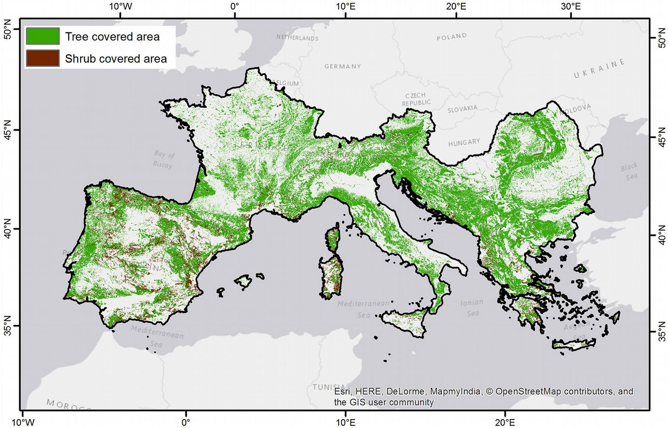
The first step in our analysis involved delineating a domain representing the Euro-Mediterranean region study area. This domain was expanded to include some countries, which did not directly border the Mediterranean Sea (Fig. 1) to guarantee all species included in the study maintained distribution continuity in terms of landscape attributes. The study area covered ~2.34 Mkm2 (24° to 50° N, 10° W to 30° E), more than 30% (801 kkm2) was covered by forests, and less than 5% (105 kkm2) supported shrubs ([7]). In total, the domain included 18 countries (Albania, Andorra, Austria, Bosnia and Herzegovina, Bulgaria, Croatia, France, Greece, Italy, Republic of Macedonia, Montenegro, Portugal, Romania, San Marino, Serbia, Slovenia, Spain and Switzerland). Administrative boundaries were included as national policy plays a vital role in protection and reforestation of forest species.
Fig. 1 - Distribution of forestlands and shrublands in the study area (black boundaries) according to FAO Global Land Cover SHARE.
Dataset and processing
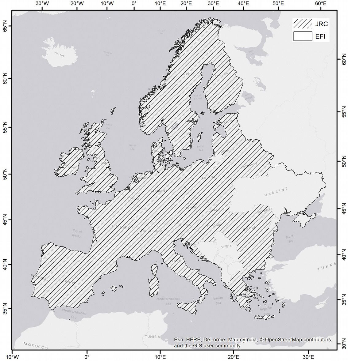
Our primary objective was to create a base dataset including forest presence data for the entire study area, with homogeneous information and spatial resolution across the study domain. The lack of homogeneity resulted in the exclusion of several national and sub-national datasets from the 18 countries considered, and in some cases, shortage of forest presence data at (sub)national levels. Review and analysis of available literature ([29]) enabled to identify the two following European datasets: (i) the European Forest Institute (EFI) “Tree species maps for Europe” ([2]); (ii) and the Joint Research Center (JRC) “Novel Maps for Forest Tree Species in Europe” ([14]). Both datasets were based on ICP-Level I plot data, with the EFI dataset derived from 1997 to 2005 data and the JRC dataset from 2000. Datasets were generated in raster format with a 1 × 1 km cell size; presence data were scaled between 0 and 100 to indicate the percent cover of each forest category type included. In addition to the similarities, the following differences were noted between the two datasets (Tab. 1): the EFI data distinguished 20 forest macro classes and covered the entire study area; the JRC data provided detailed information for 115 species, yet some study area countries were not included. The full coverage of both datasets is depicted in Fig. 2.
Tab. 1 - Main differences between EFI and JRC dataset. (*): ⇒ http://icp-forests.net/page/largescale-forest-condition.
| Parameter | EFI | JRC |
|---|---|---|
| % of cover of study area | 100 | ~90 |
| Reference years | 1997-2005 | 2000 and previous |
| Spatial resolution | 1 km | 1 km |
| Presence data format | 0-100 percentage | 0-100 percentage |
| Data sources | EFISCEN database and other National Inventories - ICP Forest Level I |
ICP Forest Level I* |
| Spatialization methods | Logistic Regression model, Kriging |
Inverse Distance Weighted Interpolation |
| Level of detail | 3 Groups, 14 Genus, 3 Species | 115 Species |
The JRC dataset alone included more detailed data regarding each species, however it did not provide the spatial continuity required in the analysis; alternatively, the EFI dataset alone provided data grouped by macro classes, while covering the entire study area. The JRC dataset exhibited the absence of presence data for five countries (Fig. 2), necessitating the integration with the EFI dataset. Thus, the two datasets were merged and the complete study area coverage was achieved for the geostatistical analyses. The following two preliminary steps were conducted prior to merging the two datasets: (i) compatibility of forest categories was accomplished; and (ii) the dataset consensus values were verified throughout the study area.
A preliminary analysis was carried out to associate EFI forest macro classes with JRC forest species. For example, the EFI category “Abies spp.” was assumed equivalent to JRC “Abies alba”, because other Abies within the study area were not reported or were geographically marginal. The same conclusions were made for EFI classes “Castanea spp.”, “Fagus spp.”, “Larix spp.”, and “Picea spp.”, which were associated with JRC classes “Castanea sativa”, “Fagus sylvatica”, “Larix decidua”, and “Picea abies”, respectively. Unfortunately, such harmonization was not feasible for all species; therefore, only 10 forest species/ classes were harmonized between the two datasets and used in this study: (1) Abies alba; (2) Betula sp. (Mediterranean Betula species); (3) Castanea sativa; (4) Fagus sylvatica; (5) Larix decidua; (6) Picea abies; (7) Pinus pinaster; (8) Pinus sylvestris; (9) Quercus robur/petraea; (10) Quercus sp. (Mediterranean Quercus species, except Q. robur and Q. petraea)
A “consensus” analysis was carried out to test the consistency of the values of species/class presence throughout the EFI and JRC geographic area datasets. Any intrinsic inaccuracies of the two datasets (due to the different methodology adopted - see Tab. 1) were evaluated by reclassifying each value (excluding those where EFI and JRC exhibited zero values) into three “semi-quantitative” presence categories for each defined species/class (low, medium, and high) using the Jenks’s natural breaks algorithm ([13]) on their frequency distribution. Finally, the two reclassified datasets were compared to verify the consensus level. On average, 85% of grid cells showed “high” consensus between datasets, with the minimum (73%) observed for A. alba and the maximum (91%) for Q. robur/petraea.
A composite 1 × 1 km cell size raster layer covering the entire study domain was then created using the JRC data for the available countries and the EFI data in the remaining areas. The raster data were entered into an ESRI® File Geodatabase for all analyses. All layers were projected in a Lambert Azimuthal Equal Area (ETRS LAEA - EPSG 3035) system.
Grid analysis and algorithm implementation
Initially, we intended to perform the spatial analysis and generate hot spot maps using CORINE Land Cover 2006 polygons as a binary forest mask (Forest Classes 3.1 and 3.2 based on the second level CORINE legend - ⇒ http://www.eea.europa.eu/data-and-maps/data/clc-2006-vector-data-version-3) to identify hot spots on actual forested areas of the study domain. Preliminary tests excluded this approach, due incompatibility of the spatial resolution between forest presence data (1 × 1 km) and CORINE (more spatially accurate - [29]). Therefore, to prevent over- and underestimate inaccuracies and provide statistical robustness for further analyses, a 10 × 10 km pixel size was selected as mapping unit, and the corresponding regular grid created in ArcGIS® shape file format. The grid was composed of 24.867 cells, and the average presence data was calculated in each cell for each species/class.
The Getis-Ord algorithm, also called “Gi* statistic” ([9], [21]) was used for hot spot analysis ([8]). The Gi* statistic indicates whether features (spatial entities) with high or low presence values tend to cluster in a geographic area, considering features within a given distance. As already mentioned, the identification of hot spots is based on the occurrence of grid cells with high values for a specific attribute surrounded by other cells with high values for that attribute. In this context, isolated cells showing a large value for a specific feature are considered outliers. The local sum for a feature in the neighborhood of a grid cell is compared proportionally to the sum of all features using Gi*; when the local sum shows a significant departure from random expectation, the result is a statistically significant Z-score (the Gi* statistic). The algorithm used for estimate Gi* statistic is represented by eqn. 1:
where xj is the average presence data for the forest category in the j-th grid cell, n is the number of neighboring cells surrounding cell i within a radius d (threshold distance), X is the mean presence data of all neighboring cells; s is the standard deviation of the presence data within d; and wij is the spatial weight between central cell i and neighboring j. ranging from 1 to 0 as a function of d.
Calculation of Gi* statistic was carried out using the “Hot Spot Analysis” tool available in the ESRI ArcGIS® software package.
Identification of threshold distances
The threshold distance is the maximum distance up to which two geographic entities (and their attributes) are related ([9]). In this study, three different threshold distances (d) were used in the Getis-Ord’s algorithm (eqn. 1) for hot spot analysis. Two predefined distances (25 km, local scale - 500 km, regional scale) were common to all the forest species/classes analyzed, while the third threshold distance (“intermediate”) was species/class-specific and was established in the range 25-500 km based on the spatial autocorrelation analysis of grid cells using the Global Moran’s I index ([19], [11] - eqn. 2):
where I is the Moran’s spatial autocorrelation coefficient, n is the number of features in the study region (in our case 10 × 10 km cells), J is the number of joins (related features), x is the attribute value (ordinal or interval) for the study area (here the average forest presence in the cell); x is the mean of all values of the variable x, and xi and xj are attribute values for two contiguous areas. The values (xi- x)·(xj- x) are calculated for each pair of contiguous areas and then summed. This index varies between 1 (complete spatial correlation) and -1 (total spatial dispersion). A zero value indicates random distribution.
The statistical significance of departure from random distribution in each distance class was obtained by calculating the Z-score ([20] - eqn. 3):
where I is the Moran’s index (see eqn. 2), -E[I]= -1/(n-1) and V[I]=E[I]2-E[I2]. When the Z-score value falls outside the confidence intervals (which depend on the significance level chosen), Moran’s index is significantly different from random expectation. In this case, I>0 indicates a clustered pattern for the set of features considered, while I<0 indicates a dispersed pattern ([23]).
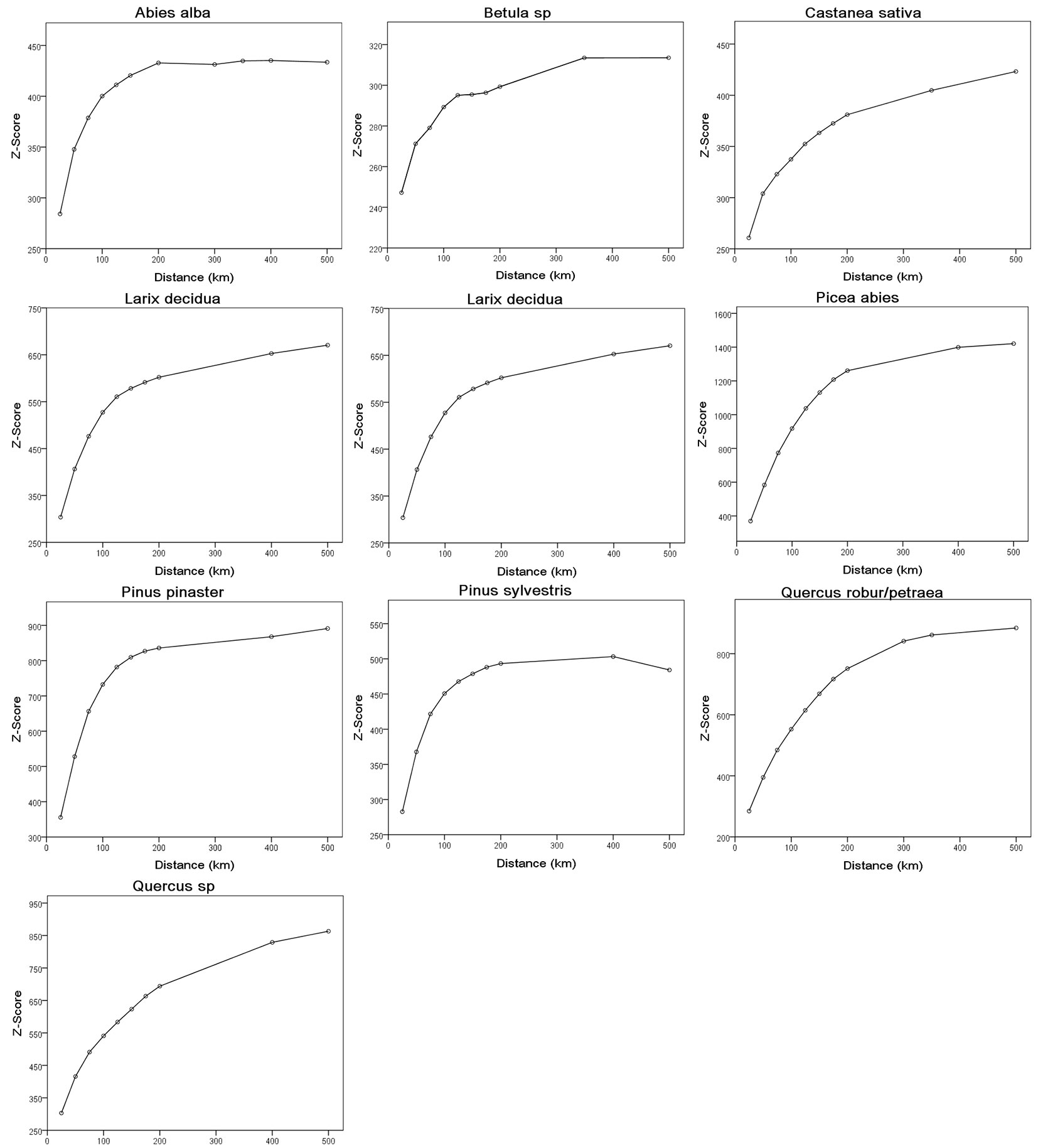
Differences among results obtained at multiple scales were evaluated by computing the Z-score values for a set of 10 incremental distances falling within the aforementioned outer limits (25, 50, 75, 100, 125, 150, 175, 200, 300 and 500 km). The Z-score graphs at increasing distances for each forest species/class are shown in Fig. 3. The best-fit function of the observed Z-score curves was calculated for each class; derivatives (tangent) of the best-fitting function along the curve were obtained, and the intermediate threshold d to be included in the Getis-Ord’s algorithm (eqn. 1) was set at the closest distance with the highest derivative value (steep slope), i.e., the distance at which spatial clustering was most pronounced (Tab. 2).
Fig. 3 - Trends of Z-score with distance for the different forest species/classes analyzed in this study.
Tab. 2 - Intermediate distances d calculated for each forest species/class and related Z-score. p-value is the probability of random distribution of the features analyzed across the study area (null hypothesis).
| Forest Class | Distance (km) |
Z-score |
Global Moran’s I |
p-value |
|---|---|---|---|---|
| Abies alba | 100 | 400.19 | 0.27 | 0.00 |
| Betula sp. | 50 | 347.72 | 0.43 | 0.00 |
| Castanea sativa | 175 | 372.54 | 0.17 | 0.00 |
| Fagus sylvatica | 75 | 466.57 | 0.40 | 0.00 |
| Larix decidua | 125 | 560.58 | 0.32 | 0.00 |
| Picea abies | 175 | 1207.85 | 0.52 | 0.00 |
| Pinus pinaster | 100 | 732.46 | 0.50 | 0.00 |
| Pinus sylvestris | 150 | 478.64 | 0.24 | 0.00 |
| Quercus robur/petraea | 175 | 716.87 | 0.31 | 0.00 |
| Quercus sp. | 100 | 540.92 | 0.37 | 0.00 |
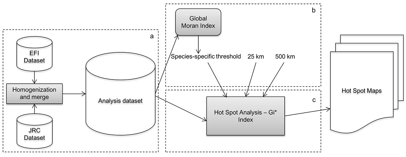
Fig. 4 provides a schematic representation of the entire methodology applied to hot spot identification. In summary, the EFI and JRC datasets were merged into a single raster dataset. The Global Moran’s Index I was used to test if species/class were randomly distributed and identify high-level hot spots, and hot spot analyses were conducted to resolve the distribution of hot spots within the study area. Finally, hot spot maps were generated for different species/classes at different threshold distances.
Fig. 4 - Flow chart of the analysis chain in (a) the datasets merging process, (b) the identification of the threshold distances and (c) the Hot Spot Analysis.
Bioclimatic analysis of hot spots
The consistency (and representativeness) of the hot spot areas identified with the climatic conditions found in each species/ class range was tested by comparing the annual and intra-annual climate conditions of hot spots with those of the entire study domain and of the whole forest class distribution reported by EUFORGEN ([6]).
Climate conditions for the entire study area were derived from the E-OBS v11.0 daily gridded dataset (⇒ http://www.ecad.eu/download/ensembles/download.php). Only air temperature and precipitation over the period 1971-2000 were considered. The 30-year average of annual and seasonal (winter, spring, summer, fall) values were calculated for each grid point. Subsequently, three different datasets including the above climatic means were created for each species/class by sampling the grid points falling into: (i) the “high” hot spots identified in this study; (ii) the whole forest class distribution domain reported by EUFORGEN ([6] - henceforth: EUFORGEN); (iii) the whole study area (study domain).
The Mann-Whitney U test (α = 0.01) was applied to test if the values of climatic variables were significantly different among the three datasets for each forest species/ class considered.
Results
Values of the Getis-Ord (Gi*) statistics were calculated in ArcGIS for each of the ten forest classes using the three threshold distances; for each distance, the Gi* statistics (represented by the Z-score value) was assigned to each grid cell. Two map series were generated: the first map series (Fig. 5) included grid cells with Z-score for each threshold distance exceeding the 95% confidence interval (CI); and the second map series selected (Fig. 6) contained grid cells with Z-score exceeding the 99% CI. We accepted these grid cells as hot spots at two different importance levels (95% CI = “high” and 99% CI = “very high”) for each forest classes. Obviously, 99% CI hot spot maps included a subset of the grid points displayed in the 95% CI maps. The 95 and 99% CI Z-score values were correlated with the threshold distances (Tab. 3). As expected, the 95% CI Z-score values increased with increased distance and ranged from 1.95 (Larix at 25 km) to 53.97 (Picea at 500 km). Likewise, the 99% CI Z-score values showed the same trend, ranging from 12.95 (Fagus at 25 km) and 81.22 (Picea at 500 km).
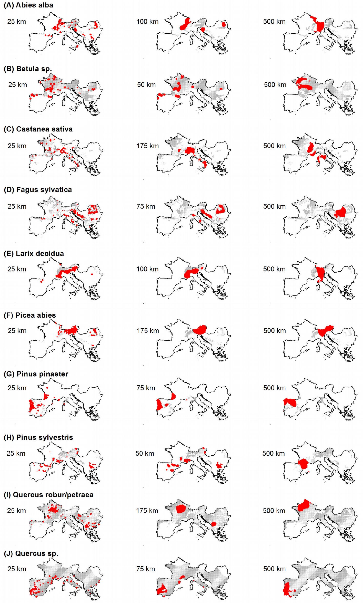
Fig. 5 - Maps showing the locations (in red) of the “high” hot spots (grid cells with Z-score above the 95th percentile) identified using the minimum (left), intermediate (center) and maximum (right) threshold distances in the hot spot analysis. Grey area represents the species distribution after EUFORGEN ([6]).
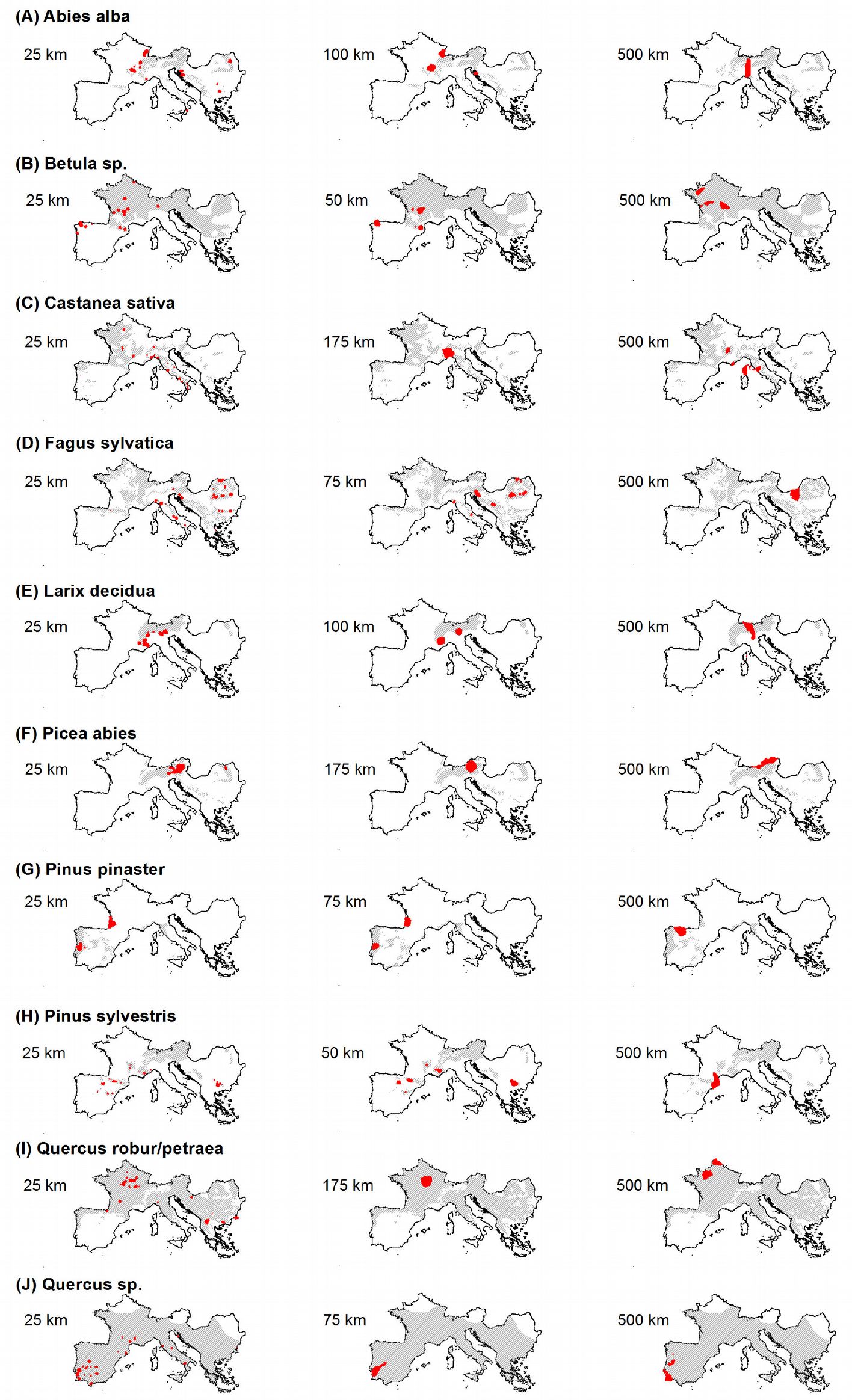
Fig. 6 - Maps showing the locations (in red) of the “very high” hot spots (grid cells with Z-score above the 99th percentile) identified using the minimum (left), intermediate (center) and maximum (right) threshold distances in the hot spot analysis. Grey area represents the species distribution after EUFORGEN ([6]).
Tab. 3 - Confidence intervals (95th and 99th percentile values) of Gi* Z-score.
| Forest class | Distance (km) | Z-score 95 perc | Z-score 99 perc |
|---|---|---|---|
| Abies alba | 25 | 4.68 | 16.62 |
| 100 | 15.48 | 27.05 | |
| 500 | 21.28 | 27.55 | |
| Betula sp. | 25 | 2.33 | 15.25 |
| 50 | 6.14 | 18.30 | |
| 500 | 18.48 | 20.33 | |
| Castanea sativa | 25 | 4.79 | 16.62 |
| 175 | 15.67 | 30.21 | |
| 500 | 21.70 | 24.28 | |
| Fagus sylvatica | 25 | 7.50 | 12.95 |
| 75 | 15.77 | 22.28 | |
| 500 | 33.98 | 43.29 | |
| Larix decidua | 25 | 1.95 | 19.05 |
| 100 | 16.08 | 41.18 | |
| 500 | 36.37 | 40.01 | |
| Picea abies | 25 | 8.04 | 19.26 |
| 175 | 39.01 | 81.22 | |
| 500 | 53.97 | 63.89 | |
| Pinus pinaster | 25 | 4.78 | 17.51 |
| 75 | 11.77 | 43.24 | |
| 500 | 39.02 | 51.29 | |
| Pinus sylvestris | 25 | 6.71 | 15.16 |
| 50 | 11.06 | 20.61 | |
| 500 | 18.99 | 27.83 | |
| Quercus robur/petraea | 25 | 6.81 | 13.29 |
| 175 | 26.92 | 41.67 | |
| 500 | 34.90 | 39.38 | |
| Quercus spp. | 25 | 7.65 | 13.11 |
| 75 | 14.70 | 24.01 | |
| 500 | 41.11 | 43.64 |
Overall, one or more protected areas were identified within 72.9% of “high” hot spots identified by the 25 km threshold, (the shape file of protected areas was obtained from ⇒ http://www.protectedplanet.net); the percentage changed to 68.31% for intermediate and 64.42% for 500 km threshold distances. However, it was notable that protected areas were present in 75.61% of “very high” hot spots identified by the 25 km threshold, in 68.51% identified by intermediate thresholds, and in 66.70% identified by the 500 km threshold. The percentage of forest classes where more than one forest class hot spot was detected, organized by thresholds and CIs is reported in Tab. 4.
Tab. 4 - Overlapping forest classes hot spots. (N): Number of overlaying classes.
| Percentile | Threshold (km) | % | N |
|---|---|---|---|
| 99th | 500 | 5.24 | 2 |
| intermediate | 0.94 | 2 | |
| 25 | 1.6 | 2 | |
| 95th | 500 | 5.13 | 3 |
| 11.56 | 2 | ||
| Intermediate | 0.01 (1 cell) | 4 | |
| 1.72 | 3 | ||
| 18.5 | 2 | ||
| 25 | 0.6 (6 cells) | 5 | |
| 1.25 | 4 | ||
| 7.95 | 3 | ||
| 20.51 | 2 |
Bioclimatic conditions for the identified “high” hot spots in each forest class, threshold distance, and climatic variables are reported in Tab. S1 and Tab. S2 in Appendix 1. In addition, the P-values obtained from the Mann-Whitney U tests to determine if the climatic variable analyzed were significantly different between the three domains considered, are provided (Tab. S1 in Appendix 1).
Overall, the EUFORGEN dataset was significantly different from the study domain dataset in 96% of cases (combinations of 10 forest classes and 10 climatic variables). Indeed, temperature and precipitation variables differed in 90-100% of cases, with the exception of C. sativa, where fall and annual temperature did not well characterize the class environment, and Quercus spp. for spring and annual precipitation.
The comparison of bioclimatic conditions of the study domain dataset with that of the “high” hot spots indicated similar temperatures in 80% (for the 500 km threshold) to 90% (for the 25 km threshold) of 15 variable combinations (given by 10 forest classes and 5 temperature parameters), with a lesser influence of seasonal temperature. Therefore, in 80% of cases (15 combinations of 5 temperature parameters and 3 threshold distances, hot spots climatic parameters did not significantly differ from the climatic conditions observed throughout the study domain. In addition, largely weak results were observed for C. sativa. Considering the 30 “forest class by threshold” combinations, various temperature parameters appeared to exhibit equal influence in hot spot distributions: slightly lower is the significance of the differences for summer, fall and annual average temperature (83% of cases), and higher for the winter (87%) and spring (90%) one.
Precipitation showed a slightly reduced influence, where significant differences between the two datasets were observed in 73% of the “forest class by threshold” combinations for winter precipitation and in 93% for spring precipitation. Using other thresholds, hot spots precipitation parameters were significant different, from 78% (25 km threshold) to 86% (intermediate thresholds). At forest class level, the combinations among precipitation parameters and threshold distances was non-significant in 60% of cases for Pinus sylvestris and Quercus robur/ petraea.
Results obtained by the comparison between “high” hot spots and EUFORGEN data were well resolved, with hot spot temperature parameters significantly different from 63% of cases (spring temperature) to 87% (winter temperature) of the “forest class by threshold” combinations. Overall, local scale hot spots (based on the 25 km threshold distance) exhibited fewer significant cases (58%) than intermediate and large scale cases (74 and 90%, respectively). Precipitation exhibited the least influence on hot spot geographic distribution, even if each precipitation-related parameter explained almost one half of the hot spots, from 50% of the fall and winter precipitation to 77% of the summer precipitation. The local, intermediate, and regional scale hot spots appeared geographically influenced by precipitation conditions in 58, 66, and 50% of combinations, respectively.
Discussion
Results obtained using the maximum threshold distance (500 km) in hot spot analysis allowed to identify large, unique, clustered areas, which might be considered representative hot spots for the entire Euro-Mediterranean domain (Fig. 5, Fig. 6c). For Abies alba hot spots were identified on the mountain ranges of central-western Europe, for Betula spp. in north-central France, in the Carpathians for Fagus sylvatica, and in the eastern Alps for Picea abies. Pinus pinaster and Quercus spp. exhibited hot spot areas in the Iberian Peninsula, the former species in the north and the latter in the south, likely due to the increased presence of other Mediterranean oaks in the region like Q. ilex and Q. suber. A hot spot for Pinus sylvestris, was identified in the Pyrenean area, while the French Normandy region was the most relevant hot spot for the mesic oak class (Q. robur/ petraea). The chestnut (Castanea sativa) is more interesting; hot spot areas exhibited increased fragmentation into several macro areas in south-central France and central Italy. The latter takes on notable importance, if we consider disease that impacted this species during the last decade ([30]).
The shortest threshold distance considered in this study (25 km) allowed to delineate a large number of local-scale hot spot areas. The results of this analysis fairly agree with previous studies. For example, based on population genetic analysis, Liepelt et al. ([15]) identified several refugia (starting points of post-glacial colonization) of Abies alba located in the Dinaric and Slovenian Alps ([4], [27]), Balkans and southern Italy (Calabria). The same areas were identified as hot spots in our study. Furthermore, hot spots for Betula spp. were localized in France (Central Massif), northern Spain (Galicia, Eastern Cantabrian mountains) and Italy (Valtellina). As for Fagus sylvatica, hot spots were identified in the Carpathians (e.g., Izvoarele Nerei Natural Reserve), in the Balkans (Sinite Kamani and Central Balkans national parks), along the Apennines (Central Liguria; Alpi Apuane Natural Park; National Park of Abruzzo, Lazio and Molise; National Park of Appennino Lucano), in the oriental Alps (Resia valley) and in the Dinaric Alps (Risnjak National Park and Velika Kapela). Most of these areas are indicated as important refuges of post-glacial recolonization for the species ([17]). For Larix decidua, we identified hot spots in the Western Alps, the Rhaetian Alps, the Dolomites and in a large area in the Prealpes of Diois (France). Hot spot areas for Picea abies were concentrated in the Eastern Alps (from Dolomites to Vienna and northern side of Salzach river valley) and some smaller areas in the eastern Carpathians. For Pinus pinaster, two areas were identified in central Portugal (Coimbra and Serra da Estrela Natural Park) and in Gascony (France). For Pinus sylvestris, the numerous areas identified as hot spots were small and localized in four macro areas: Pyrenees (e.g., Ordesa National Park) and Iberian System (e.g., Lagunas Glaciares de Neilla Natural Park), Central French Massif (southern side of Lovradois-Forez Natural Park), Maritimes Alps (Regional Park of Verdon) and the Western Rhodope Mountains. As for mesic oaks class (Quercus robur/petraea), several small areas were detected, mostly in Burgundy, in the Regional Park of Causses of Quercy (France) and in Central France, in western Macedonia, in the portion of the Basque Pyrenees, in south eastern Bulgaria and in central Slavonia (Croatia). For the remaining species of the genus Quercus (the Quercus sp. class), very small areas scattered in southern Spain and Portugal, Catalonia in Spain, Provence in France and the central and southern Apennines in Italy were identified.
The intermediate threshold distance obtained by spatial autocorrelation analysis varied between 50 km (Betula spp.) and 175 km (Castanea sativa, Picea abies and Quercus robur/petraea). Using such distance in the hot spot analysis, unique and large hot spot areas were obtained, similar to those generated by using the maximum threshold distance. In particular, isolated areas in the Jura mountains and in the French Alps were delineated for Abies; for Betula, three different regions were identified (Galicia, Eastern Pyrenees and the large area that includes the French regional parks of Millevaches en Limousin and des Volcans d’Auvergne); a region across Piemonte and Liguria (Italy) was identified as hot spot for Castanea. There were several hot spots for Fagus, such as the Ligurian Apennines, the regional park of Sirente-Velino (Central Italy), the karst plateaus of Slovenia and Croatia, the central Bosnian mountains (Sarajevo) and many Carpathians areas. For Larix Cottian, Alps and Dolomiti were detected as relevant hot spots. Picea had an extreme hot spot in the Salzakammergut Alps; Pinus pinaster in Aquitania (France) and Coimbra (Portugal); mesic oaks in Burgundy (France), and the other Quercus species in a large area from Lisbon to Extremadura (Portugal). More complex results were obtained for Pinus sylvestris: five hot spot areas were identified, among which are the Rila massif (Bulgary), the Alpes of the Haute-Provence, the department of Haute-Loire (France), the Pyrenees of Aragona and the province of La Rioja (Spain).
The bioclimatic analysis of hot spots showed that most species occur in a colder range within the study domain and in the warmer portions of their EUFORGEN range . The exception were Quercus spp. and Fagus sylvatica that seem to prefer respectively warmer and colder areas within both the study domain and EUFORGEN, and Pinus pinaster that seems more influenced by precipitation, as it preferentially occurs in wetter parts of both the whole study domain and EUFORGEN. Precipitation also appears to affect (to some extent) the hot spots geographic distribution of Fagus sylvatica, Larix decidua, and Pinus sylvestris, which occur in wetter regions of the study domain, but in the drier ones within the EUFORGEN. Both Betula spp. and Pinus pinaster showed preference for the wetter parts of the whole study domain and EUFORGEN. As expected, the variation of environmental characteristics scarcely explained the geographic distribution of Castanea sativa (largely used across Europe both for timber and fruit production) and Picea abies (used for timber). Indeed, the spread of these species is largely driven by anthropic activities. Moreover, Castanea sativa seems to occur more frequently in rainy areas of both the study and EUFORGEN domains, regardless their temperature regime. This evidence may support the choice of appropriate areas for the species’ plantation.
Concerning Picea abies and Pinus pinaster, they occur respectively in colder-wetter and warmer-wetter ranges of the study domain. Regarding these species and EUFORGEN, results showed a very poor statistical significance, likely due the high percentage of overlapping between their hot spots and EUFORGEN domain (about 60%).
The hot spot areas identified using the 25 km threshold distance largely overlap with currently protected areas (72.9 % and 75.6 % for “high” and “very high” hot spot, respectively). The remarkable decrease in overlapping percentages with increasing threshold distance (corresponding to the scale of the analysis) suggests that current conservation and protection policies are still highly locally oriented, lacking of a broader territorial perspective.
The methodology applied in this study has proved to be effective in delineating hot spot areas based on presence data. Moreover, spatial autocorrelation analysis was used to define species-specific threshold distances to be used in map production. Our results highlight the importance of applying a multi-scale approach instead of using predefined set of distances. Furthermore, the species-specific thresholds found in this study largely varied across the forest species/classes, suggesting that each species/ class needs a tailored and proper analysis in order to obtain meaningful information at the different scales of analysis.
The results presented here can be helpful to a multiplicity of end-users (e.g., local and European policy makers, practitioners, researchers, etc.). The regional, sub-regional and local hot spot maps obtained in this study may be considered a useful baseline for further ecological and economic evaluations, and to appropriately prioritize areas of interest for protection or restoration activities.
Acknowledgements
We acknowledge project funding by the Italian Ministry of Education, University and Research (MIUR) through the project GEMINA. All the datasets presented in this study are available upon request to the authors.
References
Gscholar
Gscholar
CrossRef | Gscholar
CrossRef | Gscholar
CrossRef | Gscholar
CrossRef | Gscholar
Gscholar
Authors’ Info
Authors’ Affiliation
Alessio Collalti
Riccardo Valentini
Monia Santini
Impact on Agriculture, Forests and Ecosystem Services Division (IAFES), Euro-Mediterranean Center on Climate Change (CMCC), Viterbo (Italy)
Corresponding author
Paper Info
Citation
Noce S, Collalti A, Valentini R, Santini M (2016). Hot spot maps of forest presence in the Mediterranean basin. iForest 9: 766-774. - doi: 10.3832/ifor1802-009
Academic Editor
Matteo Garbarino
Paper history
Received: Aug 11, 2015
Accepted: Jun 10, 2016
First online: Jun 13, 2016
Publication Date: Oct 13, 2016
Publication Time: 0.10 months
Copyright Information
© SISEF - The Italian Society of Silviculture and Forest Ecology 2016
Open Access
This article is distributed under the terms of the Creative Commons Attribution-Non Commercial 4.0 International (https://creativecommons.org/licenses/by-nc/4.0/), which permits unrestricted use, distribution, and reproduction in any medium, provided you give appropriate credit to the original author(s) and the source, provide a link to the Creative Commons license, and indicate if changes were made.
Web Metrics
Breakdown by View Type
Article Usage
Total Article Views: 52643
(from publication date up to now)
Breakdown by View Type
HTML Page Views: 42615
Abstract Page Views: 3909
PDF Downloads: 4659
Citation/Reference Downloads: 71
XML Downloads: 1389
Web Metrics
Days since publication: 3620
Overall contacts: 52643
Avg. contacts per week: 101.80
Article Citations
Article citations are based on data periodically collected from the Clarivate Web of Science web site
(last update: Mar 2025)
Total number of cites (since 2016): 25
Average cites per year: 2.50
Publication Metrics
by Dimensions ©
Articles citing this article
List of the papers citing this article based on CrossRef Cited-by.
Related Contents
iForest Similar Articles
Review Papers
Remote sensing-supported vegetation parameters for regional climate models: a brief review
vol. 3, pp. 98-101 (online: 15 July 2010)
Review Papers
Accuracy of determining specific parameters of the urban forest using remote sensing
vol. 12, pp. 498-510 (online: 02 December 2019)
Review Papers
Remote sensing of selective logging in tropical forests: current state and future directions
vol. 13, pp. 286-300 (online: 10 July 2020)
Research Articles
Evaluation of hydrological and erosive effects at the basin scale in relation to the severity of forest fires
vol. 12, pp. 427-434 (online: 01 September 2019)
Technical Reports
Detecting tree water deficit by very low altitude remote sensing
vol. 10, pp. 215-219 (online: 11 February 2017)
Research Articles
Geostatistical techniques for estimating aboveground biomass in eastern Amazonia
vol. 19, pp. 85-93 (online: 13 March 2026)
Review Papers
Remote sensing support for post fire forest management
vol. 1, pp. 6-12 (online: 28 February 2008)
Research Articles
Afforestation monitoring through automatic analysis of 36-years Landsat Best Available Composites
vol. 15, pp. 220-228 (online: 12 July 2022)
Short Communications
Local spread of an exotic invader: using remote sensing and spatial analysis to document proliferation of the invasive Asian chestnut gall wasp
vol. 5, pp. 255-261 (online: 24 October 2012)
Research Articles
Assessing water quality by remote sensing in small lakes: the case study of Monticchio lakes in southern Italy
vol. 2, pp. 154-161 (online: 30 July 2009)
iForest Database Search
Search By Author
Search By Keyword
Google Scholar Search
Citing Articles
Search By Author
Search By Keywords
PubMed Search
Search By Author
Search By Keyword

