An index of structural complexity for Apennine beech forests
iForest - Biogeosciences and Forestry, Volume 8, Issue 3, Pages 314-323 (2015)
doi: https://doi.org/10.3832/ifor1160-008
Published: Sep 03, 2014 - Copyright © 2015 SISEF
Research Articles
Abstract
A broad interest exists in developing structure-based indicators to use as proxies for other attributes that are difficult to assess, such as biological diversity. Summary variables that account for stand-scale forest structural complexity could facilitate the comparison among stands and provide a means of ranking stands in terms of their potential contribution to biodiversity. We developed an index of structural heterogeneity (SHI) for beech forests in southern Italy: (i) we established a preliminary list of 23 structural variables obtained from data routinely collected in forest inventories; (ii) we quantified these variables in a set of 64 beech-dominated stands encompassing a wide range of variability in the Cilento, Vallo di Diano and Alburni National Park; (iii) we identified a core set of attributes that take into account the main sources of structural heterogeneity identified in reference old-growth forests; and (iv) we combined these core attributes into a simple additive index (SHI). We identified eight core attributes that were rescaled to the range 0 to 10 using regression equations based on raw attribute data. The SHI was calculated as the sum of these attribute scores and then expressed as a percentage. The index performance was evaluated against ten reference old-growth beech stands in the Apennines. The index ranged between 38 and 79.1 (median=59.4) and was distributed normally for the calibration dataset. The SHI successfully discriminated between old-growth (range=71.9-99.9, median=85.1) and early-mature to mature forests. Furthermore, the SHI linearly increased with stand age and was higher in multi-layer high forests than in single- and double-layer forests. However, a large variation was detected within both management types and age classes. SHI could be helpful for foresters as a tool for quantifying and comparing structural heterogeneity before and after a silvicultural intervention aimed at restoring the structural complexity in second-growth stands.
Keywords
“Cilento - Vallo di Diano and Alburni” National Park, Fagus sylvatica, National Forest Inventories, Old-growth Forests, Structural Heterogeneity Index
Introduction
The theoretical and practical relevance of the structural attributes of forest stands is being increasingly acknowledged ([17], [28]). Forest structure exerts a strong control upon biological diversity, since some structural components, such as coarse woody debris or cavity trees, provide resources and habitat for a wide range of species belonging to several taxonomic groups, such as birds, bats, insects, mosses, and lichens ([51], [6], [25]).
A broad interest exists in developing structure-based indicators to use as proxies for other attributes that are difficult to assess. Several studies have tried to quantify the diversity of forest structures in a stand through the definition of synthetic indexes. Some of these indexes were designed to rank forest stands on the basis of management intensity ([45]), developmental phases ([50]) or naturalness ([34]), while others quantify the overall forest structural complexity, also referred to as structural heterogeneity, based on several attributes ([47], [52], [23]).
Stand structural complexity is essentially a measure of the variety and relative abundance of different structural attributes in a given stand. Particular attention is usually paid to those attributes that quantify variation (e.g., standard deviation of tree diameters) because they directly describe habitat heterogeneity at the stand scale ([33], [47]). In forestry, structural heterogeneity is strictly related to the spatial pattern, size distribution and height variability of trees, whether living or dead. However, depending on the objective of the study, other sources of complexity may be taken into account; for instance, vascular flora or litter distribution may still host certain organisms, modulate the resource distribution and create patchy environmental conditions. Furthermore, structural complexity can be defined at different scales (e.g., plot, stand, forest or landscape scale), and each scale can be assumed to be important for specific categories of organisms, depending on their size, dispersal ability and overall “perception” of the physical environment.
A stand-scale index of structural complexity may facilitate the comparison of stands based on their potential contribution to biodiversity ([32], [50]), since structural heterogeneity is usually assumed to be correlated with different components of plant and animal diversity ([36], [3], [6], [48], [25]). Ideally, an index of structural complexity should be easily applied by forest and land managers, and should use data routinely collected in National Forest Inventories (NFIs) so as to be widely applicable ([13], [15]).
Ranking stands according to their structural complexity may be challenging, since even ecologically similar forest stands within the same region may accumulate complexity in different ways ([16]). Structural heterogeneity arises from the occurrence of a number of different attributes whose complex interactions make its quantification an extremely difficult task ([50]). Furthermore, the relative contribution of each structural attribute to forest complexity may vary consistently across systems. Indeed, different subsets of attributes have been used by different authors for calculating stand structural heterogeneity in different regions and forest types, and all the proposed indexes are context-dependent to some extent ([33]).
Recently, McElhinny et al. ([32]) proposed an objective and quantitative methodology for constructing an index of structural complexity that identifies key structures to take into account in a specific context. They first established a comprehensive suite of stand structural attributes. These attributes were then measured in a set of stands representing the range of conditions occurring in a given region. From the analysis of these data, they finally identified a core set of attributes that were subsequently combined into a simple additive index, in which attributes were scored according to their overall regional variability ([32]).
Here, we applied this methodology to develop a stand-scale index of structural heterogeneity for Apennine beech forests. To identify the suite of attributes to include in this index of structural heterogeneity, we first explicitly defined the main sources of structural complexity commonly reported for beech natural forests in Italy and southern Europe. We considered old-growth condition as the reference state, given that late successional forests, especially old-growth stands, are known to have a high horizontal and vertical structural diversification ([40], [4], [10], [35], [49], [42], [43], [44]).
The aim of our study was thus: (i) to develop an index of structural heterogeneity for southern Apennine beech forests; (ii) to test whether different age classes and forest management types were characterized by different levels of structural heterogeneity; (iii) to compare levels of structural heterogeneity among some well-studied reference old-growth beech stands in the Apennines and forest stands that do not display old-growth attributes.
We hypothesized that, with the exception of recently established stands, which were not considered in this work, stand structural heterogeneity increases with forest age, and differs according to the management type, with double- or multi-layered uneven-aged stands having significantly higher structural heterogeneity values than even-aged single-layered stands. We also expected old-growth to be more heterogeneous than other early-mature to mature forest stands.
Methods
Study area and data collection
Data were collected in forest stands dominated by beech (Fagus sylvatica) in the Cilento, Vallo di Diano and Alburni National Park (hereafter referred to as Cilento National Park), southern Italy (Fig. 1). We limited our analysis to beech forests since they account for almost 10% of the Italian forests (more than 1 million ha, [18]) and encompass 21.7% of the Cilento National Park. Furthermore, most of the remnant old-growth stands in southern Europe are dominated by beech. This has led to a body of knowledge being accumulated in recent years about the structure and variability of this forest type under natural dynamics ([4], [35], [49], [42], [44]).
Fig. 1 - Distribution of forests in the Cilento, Vallo di Diano and Alburni National Park. Forests (light gray), beech forests (dark gray) and location of the sampling units within the beech forests (white triangles) are shown.
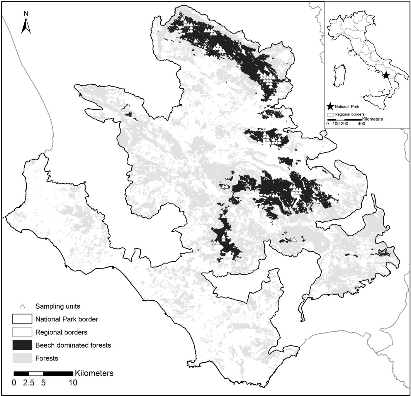
Sampling units were identified based on an aligned systematic design, overlaying a 500 m grid on the beech forest distribution map. Plots were selected with the help of the Park planning records and photo-interpretation of digital aerial photographs (Flight IT2000, nominal resolution 1 m), with a nominal scale of 1:25.000. We excluded areas whose structural heterogeneity could derive from recent harvesting, i.e., by the creation of stumps and the co-occurrence of remnant trees (or standards) and very young trees. We focused on early-mature to mature forests where structural heterogeneity is likely due to natural forest dynamics (tree senescence and death, establishment of natural regeneration and gap dynamics, etc).
Overall, 64 sampling units across 12 forest areas were selected, encompassing an area of about 137 km2 (Fig. 1). These included stands diversely managed, ranging from coppices with different standard densities, to even- and uneven-aged high forests. Some of the stands showed old-growth features, such as large old trees, logs and snags.
A circular plot of 20-m radius (1256 m2) was established in each unit. Living trees in each plot were calipered in concentric circular areas with a radius of 4, 13 and 20 m, with thresholds of minimum diameter at breast height (DBH) of 2.5, 10 and 50 cm, respectively. Height was measured using a Haglof Vertex on one out of ten sampled trees, chosen randomly. For the remaining trees, the height was estimated with a traditional H=f(DBH) model calculated on the basis of the trees whose height was measured. In the intermediate circular area (13 m radius), the length and diameter of all the lying deadwood components (with a minimum diameter ≥ 10 cm) were measured, as well as their decay level according to Hunter ([24]). The age of each stand was estimated in the field by expert opinion on the basis of evidence of past disturbance or harvest, as well as on the mean size of canopy trees. Age was assigned to one out of six broad classes (1: < 50 yrs; 2: 50-80; 3: 80-100; 4: 100-120; 5: 120-140; and 6: > 140 yrs old). Stands were classified according to their management type and structure in the following groups: single-, double-, and multi-layer high forests, and coppices. The distribution of estimated ages across forest types is reported in Fig. S4 (Appendix 4). For a more detailed description of the forest structure data collection and preliminary analysis, see Blasi et al. ([5]) and Burrascano et al. ([8]).
As an additional dataset, we selected 10 beech-dominated stands in central Italy with old-growth features (such as high density of large living trees, high amount of deadwood, uneven-aged structure), whose high structural heterogeneity was previously reported in several studies ([40], [7], [31], [43], [44], [10], [49]). Information on location, climate, underlying bedrock and time since last disturbance of these stands is provided in Tab. S1 and Fig. S1.1 (Appendix 1).
Living trees and deadwood were sampled within a 1 ha plot in all the study sites except two (Cozzo Ferriero, 0.16 ha; Fosso Cecita, 0.45 ha), in which plot size was reduced because of the very steep slopes. The position, species, DBH (minimum threshold of 3 cm) and height of every tree in the plot were recorded, as well as the position, diameter and length (or height) of standing dead trees, downed dead trees, snags and stumps. Deadwood pieces were sampled if they met the following requirements: minimum diameter > 5 cm, more than half the base of their thicker end lying within the plot, length > 1 m. Further details are reported by Lombardi et al. ([31]) and Calamini et al. ([10]).
Selection of structural variables to include in the Index
An index of structural heterogeneity was built according to the methodology proposed by McElhinny et al. ([32]). This four-stage approach starts from (i) the definition of a comprehensive suite of structural attributes that are (ii) then sampled and analyzed in order to (iii) identify a core set of attributes and (iv) combine them into an index.
We compiled a preliminary list of 23 structural variables that may easily be derived from routinely collected data in forest monitoring programmes and NFIs ([13]). This list comprised: (1) basal area; (2) growing stock; (3) number of DBH classes; (4) DBH diversity (calculated using the Gini-Simpson Index); (5) DBH range; (6) number of living trees with DBH>40cm; (7) tree species richness; (8) quadratic mean DBH; (9) living stem density; (10) height; (11) height standard deviation; (12) snags volume; (13) standing dead trees volume; (14) Total standing deadwood volume; (15) density of standing deadwood (both snags and standing dead trees); (16) basal area of standing deadwood (both snags and standing dead trees); (17) stumps volume; (18) lying coarse woody debris volume; (19) the logarithm of the sum of the lengths of lying coarse woody debris pieces (hereafter referred to as “total log length”); (20) total deadwood volume; (21) ratio between deadwood and living wood volumes; (22) number of decay classes occurring in the plot; (23) coarse woody debris index (CWDI, see Appendix 2 for calculation according to [32]).
To define the suite of attributes to be considered in the final core set of attributes, we first listed the main sources of structural complexity occurring in beech natural forests, as reported in recent literature on old-growth forests in southern Europe ([40], [4], [10], [35], [49], [30], [42], [44]). We considered above all sources of heterogeneity correlating with other desirable properties, e.g., plant and fungi biodiversity, faunal habitat availability and carbon stocking ([23], [7], [5], [48], [21], [53]). Eight sources of structural complexity were considered: (1) vertical heterogeneity; (2) compositional diversity; (3) uneven-agedness; (4) density of large living trees; (5) growing stock; (6) total deadwood volume; (7) deadwood decay classes; (8) standing dead trees and snags. A brief description of these elements and how they relate to other ecosystem properties are reported in Tab. 1.
Tab. 1 - List of the eight sources of structural heterogeneity considered in the present study and their ecological importance for forest biodiversity. This list represents the basis to select the structural attributes for constructing the SHI (Structural Heterogeneity Index).
| Sources of structural heterogeneity |
Description | References |
|---|---|---|
| Vertical heterogeneity (VH) |
Stands containing a variety of tree heights are likely to contain a variety of tree ages and, consequently, a high vertical and horizontal heterogeneity. Horizontal and vertical patterns of trees significantly affect demographic processes, resource distribution (e.g., light), and understory development. | [9], [20], [47] |
| Compositional diversity (CH) | The presence of a mix of shade-tolerant and shade-intolerant tree species may produce a multi-layered canopy. Compositionally diverse tree layers may favour herb-layer diversity, since different tree species may have different light transmittance and litter quality. | [1], [2], [8], [21] |
| Uneven- agedness (UA) |
In forested landscapes where small to intermediate scale disturbance events are dominant, an uneven-aged structure may indicate a natural development of the stand, or the application of close-to-nature silvicultural practices. The variability in tree size may also be an indicator of the diversity of niches occurring within a stand that could be used by a wealth of animal and plant organisms. | [26], [21] |
| Density of large living trees (LLT) |
Large living trees store a large amount of carbon and provide habitat functions for a number of threatened or ecologically important forest species. These functions relate to the great variety of niches that large trees offer, including rough bark, trunk hollows, exposed deadwood, sapflows, dead branches and dead tops. | [6], [39], [37] |
| Growing stock (GS) |
Higher living above-ground biomass indicates the degree to which a stand effectively accomplishes its function of storing carbon. Owing to greater levels of biomass, old-growth stands were shown to attenuate surface temperature more effectively than managed stands, hosting a higher proportion of forest specialist herb-layer species | [23], [22], [38] |
| Total deadwood volume (DW-TOT) |
Deadwood is a key ecosystem feature supporting high levels of biodiversity, for instance providing diverse niches for many specialized and saproxylic organisms. Such organisms include those with low dispersal capabilities that need long-term availability of deadwood substrate, whose absence in intensively managed stands may cause local or regional extinction of several species. | [11], [27], [53] |
| Deadwood decay classes (DW-DC) |
The absence of deadwood in one or several decay phases strongly indicates a break in the continuity of deadwood supplies, typically due to a combination of recent harvesting and deadwood removal. This may affect the continuity of nutrient supply to the forest floor, and the diversity and abundance of saproxylic organisms. | [29], [7], [27] |
| Standing deadwood, dead trees and snags (DW-ST) | Standing dead trees and snags may bear niches such as tree hollows, cavity strings and cracks that are important for a variety of species such as breeding birds, mammals and invertebrates, as well as for lichens and bryophytes. | [6], [21] |
When designing an index of structural complexity, one should focus on attributes that: (i) have a low kurtosis, since a high kurtosis would indicate similar values of an attribute for several sites; (ii) may help to distinguish between categories of interest (e.g., early- versus late-successional stands); (iii) are proxies of other variables or originally contribute to the overall structural stand complexity; (iv) are easily measurable in the field ([32], [13]).
Both logarithm and square-root transformations were applied to improve the distribution of attributes showing a high kurtosis (<2): in the selection stage, we only retained the transformation that most improved their distribution.
Since we assumed that structural complexity increases with age, early- and late-successional stands were separated choosing an age threshold of 100 years (which represents the usual harvest return interval for beech forests in the Apennines) and then compared. Differences between the two mentioned groups were tested for each structural variable by Mann-Whitney test.
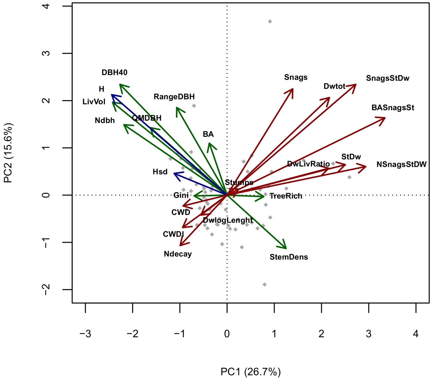
Pairwise correlation between variables was calculated using the Spearman’s ρ coefficient. To visualize the multi-correlation structure of variables and evaluate their redundancy, we performed a Principal Components Analysis (PCA) and represented it in Gabriel’s plots (only the first 2 principal components, accounting for 42.3% of the total variance, are shown in Fig. 2).
Fig. 2 - PCA of standardized structural variables, axes 1-2. (Green): Live trees structural variables; (Red): Deadwood-related variables; (Blue): Tree Height-related variables. (BA): Basal area; (RangeDBH): range of diameter distribution; (QMDBH): quadratic mean diameter; (LivVol): growing stock; (Ndbh): number of diameter classes; (StemDens): Stem density; (TreeRich): tree species richness. (CWD): Coarse woody debris volume; (Stumps): volume of stumps; (Snags): volume of standing dead trees broken above 1.3 m; (StDw): volume of standing dead trees; (SnagStDw): volume of standing dead trees (including snags); (NsnagsStDW): number of standing dead trees (including snags); (BASnagSt): basal area of standing dead trees (including snags); (DWtot): Deadwood (standing + CWD) total volume; (DWLivRatio): living wood/Deadwood volume ratio; (CWDI): coarse woody debris index (see Appendix 2); (DwlogLength): log of the sum of lengths of every coarse woody debris piece; (H): mean height; (Hsd): height standard deviation.
To help in variable selection, we also estimated whether they were more or less difficult to sample and/or calculate. Variables that only need tree diameter data (e.g., Gini-Simpson’s diversity, basal area) were considered having a sampling efficiency higher than variables requiring the estimation of other parameters, such as tree height or deadwood debris decay class. To this purpose, variables were grouped in 3 sampling efficiency classes (1: low to 3: high). When selecting between two or more highly correlated variables to be included in the index, those with a high sampling efficiency were favored (see Appendix 3).
Finally, we created a core set of structural attributes that included a variable for each of the eight sources of structural complexity listed in Tab. 1. Considering the first source of structural complexity (VH), the variable best describing this feature (height standard deviation) was included, provided that it matched the four selection criteria listed above. A similar procedure was adopted for the next sources of structural complexity until all eight sources were represented in the core set. We took tha additional care that the new variable added to the set had the lowest correlation with the variables included in the previous steps. If no variable matched all the selection criteria for a given source of complexity, variables showing low kurtosis and low correlation with those already included were favored. The eight structural variables included in the core set are listed in Tab. 2.
Tab. 2 - Core set of structural variables and selection criteria. (W): Wilcoxon test (equivalent to Mann-Whitney); (Source): the source of heterogeneity indicates whether the variable could be a proxy of one of the eight features described in Tab. 1; (VH): vertical heterogeneity; (CH): composition heterogeneity; (UA): uneven-agedness; (LLT): occurrence of large living trees; (GS): high growing stock; (DW-TOT): occurrence of a relatively high deadwood volume; (DW-DC): occurrence of deadwood in different decay classes; (DW-ST): occurrence of standing deadwood, dead trees and snags. Sampling efficiency: 1 - poor, 2 - medium, 3 - high.
| Structural indicators |
Kurtosis | Medians | Function as a surrogate (significant ρ > 0.5) |
Source | Sampling efficiency |
|||
|---|---|---|---|---|---|---|---|---|
| <100 yrs (n=26) | > 100 yrs (n=38) | W | Prob. | |||||
| Living volume |
0.23 | 421.17 | 524.38 | 330 | 0.025 | Basal Area (0.53); no. DBH classes (0.53); no. trees DBH> 40 cm (0.68); Height (0.67) | GS | 1 |
| no. trees DBH>40 cm |
-0.11 | 1 | 6.5 | 186 | 0.001 | Living volume (0.66); DBH range (0.66); Height (0.78); Density of standing deadwood (-0.55); Basal area of standing deadwood (-0.50) | LLT | 3 |
| Diameter diversity (Gini-Simpson index) |
-0.81 | 0.6 | 0.72 | 575 | 0.273 | Living stem density (-0.64); Quadratic mean DBH (0.71) | UA | 2 |
| Height standard deviation | -0.34 | 3.53 | 5.47 | 321 | 0.018 | - | VH | 2 |
| CWD index | -0.99 | 2 | 2 | 516.5 | 0.754 | Lying CWD Volume (0.85); no. decay classes (0.75); Total log length (0.86) | DW-DC | 1 |
| log (Tree species richness) | 0.17 | 1.1 | 0.69 | 573.5 | 0.229 | - | CH | 3 |
| log (basal area of standing deadwood) | -0.31 | 0.85 | 0.18 | 323.5 | 0.018 | Height (-0.50); Snags volume (0.68); Standing dead trees volume (0.86); Total Standing deadwood (0.98); Total deadwood (0.73); Density of standing deadwood (0.89); Dead/Living wood ratio (0.76) | DW-ST | 3 |
| sqrt (total deadwood) | 0.04 | 4.7 | 4.63 | 526.5 | 0.662 | Standing dead trees volume (0.65); Total Standing deadwood (0.77); Density of standing deadwood (0.68); Basal area of standing deadwood (0.61); Dead/Living wood ratio (0.96) | DW-TOT | 1 |
Construction of a Structural Heterogeneity Index (SHI)
A score ranging from 0 to 10 was assigned to each attribute in the core set based on linear regression through quartiles (Tab. 3). We first set a score of 2.5, 5, 7.5 and 10 to the quartile midpoints (corresponding to the 12.5, 37.5, 62.5 and 87.5 percentiles, respectively) of the raw attribute distribution. Then, a linear regression through quartile values was fitted to ensure that the attribute scores were evenly distributed between 0 and 10. This regression equation was used to associate a score with each observation. Regression was constrained between 0 and 10 to prevent extremely low and high values from taking scores outside the range. The maximum attribute score of 10 was attributed to the 87.5 percentile. Compared with a simple scaling of values in the range -1 to 1, the above technique has the advantage of avoiding possible distortions due to the occurrence of extremely high or low outliers, and yielding a more even distribution of index scores across the range of variability of the raw attributes.
Tab. 3 - Regression equations used to assign a score to attributes on a scale of 0-10, obtained from 64 beech dominated forest stands in the Cilento, Vallo di Diano e Alburni National Park, southern Italy. For more details, see Materials and Methods.
| Attribute | Regression equation | R2 |
|---|---|---|
| Living volume | Score = -2.021 + X · 0.016 | 0.938 |
| no. Large Living Trees DBH> 40 cm | Score = 3.274 + X · 0.595 | 0.952 |
| DBH diversity (Gini-Simpson index) | Score = -2.233 + X · 14.034 | 0.969 |
| Height standard deviation | Score = 1.815 + X · 0.811 | 0.918 |
| CWD index | Score = 3.750 + X · 1.25 | 0.900 |
| Log (Tree species richness) | Score = -2.511 + log(X) · 9.053 | 0.900 |
| Log (basal area of standing deadwood) | Score = 3.536 + log(X) · 4.221 | 0.924 |
| sqrt (Total deadwood volume) | Score = 1.167 + sqrt(X) · 1.083 | 0.999 |
Finally, a Structural Heterogeneity Index (SHI) was obtained by summing the scores in the range 0-10 assigned to each variable in the core set, and then expressed as a percentage. Score weighting was not considered here because: (i) it could imply an arbitrary choice; (ii) index performances were found to be independent of the weighting of attributes ([32]); (iii) an unweighted index provides a clearer picture of the relative contribution of different sources of heterogeneity.
Testing the Structural Heterogeneity Index
SHI values calculated for the 64 forest plots in the Cilento National Park were tested for significant differences between broad classes based on age and management type using non-parametric Kruskal-Wallis test. We used multiple regression to test whether the SHI significantly increases with age, and covariates with management type as well as with other environmental attributes (i.e., altitude, slope, aspect). Backwards selection was applied to discard non-significant terms.
As an additional evaluation of index performances, we calculated the SHI on the set of 10 beech-dominated, old-growth forests from central Italy (Fig. S1.1, Tab. S1 - Appendix 1), whose structural data were not used during the calibration process. SHI values of such forests were compared with those obtained for plots in early-mature to mature stands in the Cilento National Park. We tested for significant differences by means of the Kruskal-Wallis test.
All analyses were performed using the software package R 2.14.1 ([41]).
Results
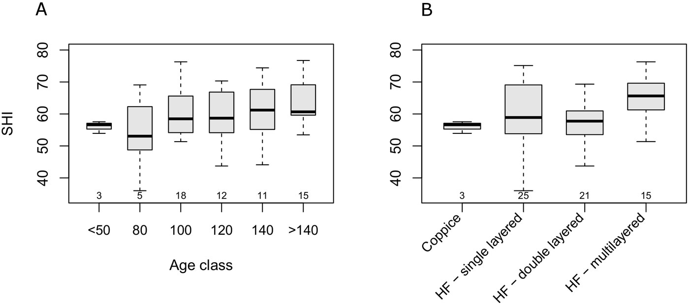
Beech stands in the Cilento National Park showed index values ranging between 38 and 79.1 (median 59.4) and showing no departure from normal distribution (Fig. S5.1). The SHI appeared to have a minimum in the 80 year-age class, and a slow increase with age (Fig. 3A). A high variability of SHI values was observed within each age class, and no significant differences among classes (Kruskal-Wallis H = 6.08, df = 5, p = 0.297). On the other hand, the SHI significantly differed across management types (H = 10.39, df = 3, p = 0.015). However, the only significant (p<0.05) difference using post-hoc multiple comparison was detected between multi-layer and double-layer high forests (Fig. 3B). Multiple regression showed a significant linear increase in the SHI with stand age (b = 0.064, t(61) = 2.48, p = 0.015) and a negative relationship with altitude (b = -0.022, t(61) = -3.31, p = 0.002). Adjusted-R2 was 0.19. Based on the above analysis, neither management type, nor the interaction between management type and age, were significant predictors of the SHI.
Fig. 3 - Boxplot of SHI across age classes (A) and structural types (B). Small numbers below the boxes represent the sample size. (HF): High forest.
Structural heterogeneity of a set of Italian beech old-growth forests
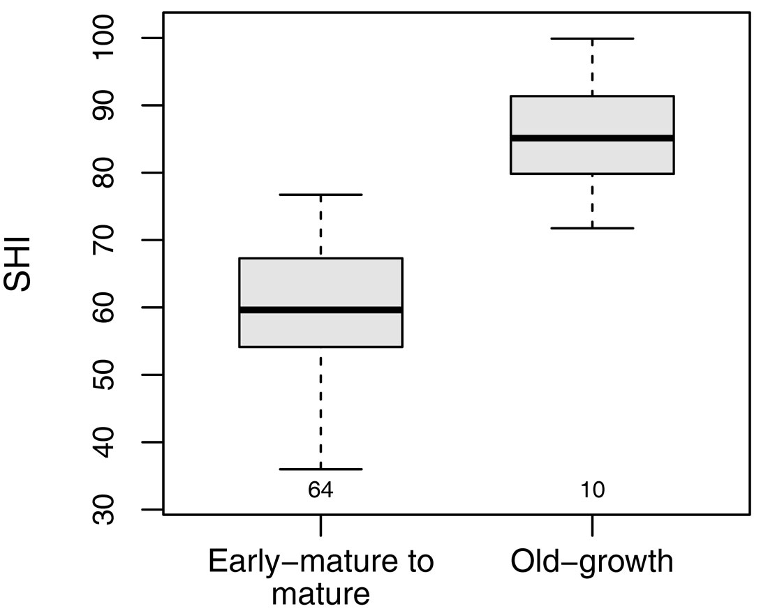
The SHI of the selected old-growth stands ranged between 71.7 and 99.9 (median 85.1). The SHI was significantly higher for reference old-growth stands than for the beech stands included in the main dataset (H = 27.7, df = 2, p < 0.001 - Fig. 4, Tab. 4).
Fig. 4 - SHI comparison between early-mature to mature, and old-growth stands. The boxplots refer to the SHI of managed beech forests in the Cilento National Park (left) with those of a set of beech forests with old-growth features located throughout the Apennines (right). Small numbers below the boxes represent the sample size.
Tab. 4 - SHI values and scores for its sub-components calculated for 10 beech stands with old-growth features located throughout the Apennines. Scores for each structural variable was obtined by the regression equations reported in Tab. 3. SHI was calculated as the sum of variable scores, normalized on a percent basis.
| Stand | Living volume |
No. trees DBH>40 cm |
DBH diversity (Gini-Simpson) |
Height sd |
CWD index |
Log (tree sp. richness) |
Log (BA stand dw) |
Sqrt (total dw) |
SHI |
|---|---|---|---|---|---|---|---|---|---|
| Abeti Soprani | 6.9 | 10.0 | 10.0 | 6.8 | 10.0 | 10.0 | 9.4 | 10.0 | 91.4 |
| Collemeluccio | 6.7 | 10.0 | 10.0 | 6.6 | 10.0 | 10.0 | 4.8 | 5.7 | 79.8 |
| Cozzo Ferriero | 10.0 | 10.0 | 10.0 | 8.4 | 10.0 | 0.0 | 7.1 | 10.0 | 81.8 |
| Fonte Novello | 10.0 | 10.0 | 10.0 | 7.3 | 10.0 | 0.0 | 10.0 | 10.0 | 84.1 |
| Gargano-Pavari | 8.4 | 10.0 | 10.0 | 10.0 | 10.0 | 7.4 | 9.1 | 10.0 | 93.7 |
| Monte Cimino | 10.0 | 10.0 | 9.3 | 10.0 | 10.0 | 10.0 | 5.0 | 7.3 | 89.5 |
| Monte di Mezzo | 9.0 | 10.0 | 10.0 | 7.8 | 10.0 | 10.0 | 5.4 | 6.7 | 86.2 |
| Monte Sacro | 5.3 | 10.0 | 8.3 | 7.9 | 10.0 | 0.0 | 5.9 | 10.0 | 71.7 |
| Sasso Fratino | 10.0 | 10.0 | 10.0 | 10.0 | 10.0 | 10.0 | 10.0 | 9.9 | 99.9 |
| Val Cervara | 3.7 | 10.0 | 8.6 | 8.6 | 10.0 | 0.0 | 10.0 | 10.0 | 76.1 |
The high SHI values observed in the old-growth stands stem from the high scores of index subcomponents, whose relative importance varied greatly across stands (Tab. 4). According to the SHI, each of the 10 old-growth stands was structurally heterogeneous in a unique way; the most important sources of SHI variability among old-growth stands were living volume, tree height standard deviation, canopy tree species richness and basal area of standing deadwood. For instance, living volume greatly varied across the 10 old-growth stands, probably as a result of differences in altitude, site fertility and time since last disturbance. Although “Val Cervara” is probably the best preserved old-growth beech stands in central Apennines, this stand only attained a very low score for living volume (3.7 out of 10), when compared with other stands located at lower altitudes and in more favorable site conditions (e.g., “Fonte Novello” or “Monte Cimino”). The basal area of standing deadwood also strongly varied across stands (from 4.8 in “Collemeluccio” to 10 in “Fonte Novello”, “Sasso Fratino” and “Val Cervara”). Species richness of the tree layer varied markedly and clearly distinguished between pure beech stands (e.g., “Fonte Novello”, “Val Cervara”) and beech stands mixed with other taxa such as Abies alba (e.g., “Abeti Soprani”, “Sasso Fratino”), or other broad-leaved species, such as Ilex aquifolium and Acer obtusatum in “Gargano-Pavari”, or A. obtusatum and A. pseudoplatanus in “Monte Cimino”.
Discussion
Management, disturbance history, and environmental factors contribute to current forest heterogeneity
We applied an acknowledged methodology to obtain an index of structural heterogeneity for southern Italy beech forests. Forest structural heterogeneity, as indicated by the SHI, linearly increased with stand age and was higher for multi-layer high forests than for single- and double-layer forests.
The positive relationship between the SHI and stand age closely matched our expectations, although there was a marked variability both within management types and age classes. Such variability was likely due to the wide range of site conditions, soil fertility, disturbance and forest management histories found in the study area. In particular, the SHI revealed a very high degree of variation in single- and double-layer high forests. These management types encompassed stands with highly variable amounts of growing stock (whose index sub-scores ranged between 2 and 10 for single-layered and between 1.1 and 10 for double-layered stands), height standard deviations (scores ranging between 2.6-10 and 3.3-10, respectively) and coarse woody debris volumes (1.1-10 and 1.1-9.4, respectively).
Although part of this variability can be accounted for by differences in age classes and altitude, the relationship observed between stand age and complexity should be considered only as a general trend. Since the management history of most stands is only partially known (harvest archives in most municipalities of the study area date back no longer than the 1990s), stands were only classified into broad age classes on the basis of expert opinion. More detailed stand age data, including accurate dendrochronological reconstructions of their past disturbances, would be required to quantify the actual rate at which forest complexity increases over time.
Besides stand age, most of the remaining variability is likely to be dependent on the different disturbance and harvesting histories of these stands. Forests in southern Italy are characterized by a peculiar history: in the 19th century, a forest law prescribed clearcuts with the release of 45 standards per hectare to be applied indistinctly to all the forests of the Kingdom of the two Sicilies (which included southern Italy and Sicily). However, this law was never extensively applied, and most of the forests continued to be subject to selective cuttings ([19]), even well into the 20th century. Although the shelterwood system began to be applied regularly to the Apennine beech forests in the 20th century, beech forests in southern Italy have been frequently managed according to models based on “local knowledge”, resulting in a wide range of silvicultural and harvesting practices that have contributed to the current variability of the forest structures in the study area.
Use of SHI for the classification of old-growth forests
In an operational context, structural indicators may prove very useful to distinguish old-growth forests from younger developmental stages, as well as to rank forests along “old-growthness” gradients ([28], [17]). However, old-growth characteristics should be defined not only on the basis of a set of structures providing desirable functions, but also based on the developmental processes producing such structures. The SHI does not discriminate the process (anthropogenic vs. natural) that resulted in a certain amount of heterogeneity accumulating in a stand. Nevertheless, we believe this index may be useful for assessing how far a stand is from reference old-growth characteristics, but only when no further information on long-term disturbance history is available.
Recently, Chiavetta et al. ([12]) have attempted to rank Italian beech forests on a scale of “old-growthness” based on the multivariate dissimilarity of studied stands from a reference virtual old-growth stand whose structural attributes were derived from the literature. In our opinion, this is an interesting approach, though suffering from the fact that literature data on old-growth structural variability is either very scarce or completely lacking for most forest types in Europe, and reference attributes had to be derived from unrelated biogeographical regions. Unlike the above approach, the SHI was only based on the structural variability observed in the study region, as suggested by McElhinny et al. ([32]), and on a list of desirable features widely recognized as important sources of heterogeneity in old-growth stands. Therefore, the SHI is less likely to be subject to bias deriving from incorrect assumptions.
In this study, old-growth stands showed very high SHI values, sometimes close to the maximum as in the case of the “Sasso Fratino” stand. This result confirmed that this index effectively captures aspects of structural heterogeneity recognized as important in reference beech old-growth forests in southern Europe ([40], [35], [42], [44]). The core set of structural attributes considered here may be further expanded including other significant sources of complexity, such as gap fraction, diversity of shrubs or other vascular plants, or litter distribution variability. However, a trade-off exists between the relevance of information included in the index and its cost in terms of time or expertise required ([13], [34]). In this study, we chose to include in the SHI only those structural variables that can easily be obtained from routinely collected data in plot-based forest inventories, with no need of vegetation surveys (e.g., understory diversity or abundance assessments) or analysis on a broader spatial scale (e.g., to estimate forest gap fraction).
Since SHI successfully distinguished between old-growth and younger stands, the question arises whether this index could also be used to assess the “naturalness” of a forest stand. The concept of “naturalness” is related to the degree to which forest ecosystems are characterized by natural processes and/or the absence of human influences ([34]). To this regard, the SHI does not include any metrics to measure human impact. In theory, very high SHI values may be obtained also for forest stands deeply modified by silvicultural practices aimed at enhancing its structural complexity. Therefore, we recommend the application of SHI only in studies aimed at assessing the structural heterogeneity of forest stands.
Potential and limitations of the SHI
There is a great need for simple tools that can help forest managers to improve stand biodiversity ([50]). To this purpose, the SHI may be useful to test the effectiveness of silvicultural practices aimed at restoring the complexity in second-growth stands, by comparing the structural heterogeneity before and after the intervention.
One of the main advantage of the SHI is that it simply consists of the sum of scores for each structural attribute, obtaining a “synthetic” index of stand complexity. On the other hand, similar SHI values may mask different underlying source of heterogeneity. This was the case of the “Abeti Soprani” and “Monte Cimino” old-growth stands (Tab. 4), sharing similar SHI values but strongly differing in attributes such as tree height standard deviation, basal area of standing deadwood and total deadwood volume. However, the additive structure of the SHI may help forest managers to assess the relative contribution of each attribute to overall stand heterogeneity, thereby helping to prioritize specific silvicultural interventions aimed at increasing forest structural complexity. This is particularly relevant in the context of adaptive management.
The SHI relies upon input data routinely acquired by almost all the NFIs in the world ([13]). Therefore, it may be appiled to stands from a wide range of biogeographical regions ([14]). So far, we tested its performance on a relatively wide set of forest stands, encompassing all the climatic, topographical and soil variability found in beech forests in the Cilento National Park. However, before its use in other contexts, we recommend a fine-tuning of the SHI on an adequately comprehensive dataset, such as that from the last Italian natio nal forest inventory ([18]).
Forest structural indicators may also be sensitive to the field methods used for their assessment, such as plot size and minimum DBH thresholds ([34], [14]). The need for harmonization procedures in the calculation of structural indexes from different field acquisitions has often been advocated ([46]). In our study, we used two different datasets that had consistently similar deadwood and living wood diameter thresholds, but a substantially different plot size (1256 m2 vs. 1 ha). This may represent a potential source of bias, though we do not expect this could severely affect our results. Indeed, data collected in small plots may provide an estimation of structural parameters less accurate than those from large plots but, as long as plots are randomly located, an unbiased estimation of structural attributes on a per hectare basis is still obtained. Such difference in precision may be particularly marked when structural attributes associated with relatively rare elements are considered, such as standing dead trees, though the estimation of the SHI will still be substantially unbiased.
In conclusion, indicators based on key structural parameters are of considerable interest as practical surrogates for attributes that are normally too expensive or difficult to measure, such as biodiversity or ecosystem functioning. The common assumption that the structural, functional, and compositional attributes of a stand are inter-dependent ([17], [21]) requires further testing. Future analyses are needed to assess the performance of the SHI outside the study area and its relationship with several important ecosystem functions, such as forest biodiversity, productivity and resilience, biogeochemical cycles or wildlife food availability.
Acknowledgements
We thank the Cilento, Vallo di Diano and Alburni National Park for funding this research and the State Forestry Corps for their assistance during the fieldwork. We also wish to thank all the colleagues who took part in the field campaign. FMS and SB conceived the study, FMS performed the statistical analysis, FL and GC provided old-growth forests data. FMS, SB, FL, GC and CB interpreted the data and contributed to the drafting of the manuscript. We would also like to thank our language reviewer Lewis Baker.
References
CrossRef | Gscholar
CrossRef | Gscholar
CrossRef | Gscholar
Gscholar
CrossRef | Gscholar
Gscholar
CrossRef | Gscholar
CrossRef | Gscholar
CrossRef | Gscholar
CrossRef | Gscholar
Supplementary Material
Authors’ Info
Authors’ Affiliation
Sabina Burrascano
Carlo Blasi
Department of Environmental Biology, University of Rome “La Sapienza”, p.le Aldo Moro 5, I-00185 Rome (Italy)
Gherardo Chirici
Dipartimento di Bioscienze e Territorio, Università degli Studi del Molise, c.da F.te Lappone snc, I-86090 Pesche (IS, Italy)
Corresponding author
Paper Info
Citation
Sabatini FM, Burrascano S, Lombardi F, Chirici G, Blasi C (2015). An index of structural complexity for Apennine beech forests. iForest 8: 314-323. - doi: 10.3832/ifor1160-008
Academic Editor
Renzo Motta
Paper history
Received: Oct 22, 2013
Accepted: May 21, 2014
First online: Sep 03, 2014
Publication Date: Jun 01, 2015
Publication Time: 3.50 months
Copyright Information
© SISEF - The Italian Society of Silviculture and Forest Ecology 2015
Open Access
This article is distributed under the terms of the Creative Commons Attribution-Non Commercial 4.0 International (https://creativecommons.org/licenses/by-nc/4.0/), which permits unrestricted use, distribution, and reproduction in any medium, provided you give appropriate credit to the original author(s) and the source, provide a link to the Creative Commons license, and indicate if changes were made.

Web Metrics
Breakdown by View Type
Article Usage
Total Article Views: 62024
(from publication date up to now)
Breakdown by View Type
HTML Page Views: 48627
Abstract Page Views: 4377
PDF Downloads: 7510
Citation/Reference Downloads: 46
XML Downloads: 1464
Web Metrics
Days since publication: 4345
Overall contacts: 62024
Avg. contacts per week: 99.92
Article Citations
Article citations are based on data periodically collected from the Clarivate Web of Science web site
(last update: Mar 2025)
Total number of cites (since 2015): 29
Average cites per year: 2.64
Publication Metrics
by Dimensions ©
Articles citing this article
List of the papers citing this article based on CrossRef Cited-by.
Related Contents
iForest Similar Articles
Research Articles
Do different indices of forest structural heterogeneity yield consistent results?
vol. 15, pp. 424-432 (online: 20 October 2022)
Book Reviews
National forest inventories: contributions to forest biodiversity assessments (2010)
vol. 4, pp. 250-251 (online: 05 November 2011)
Research Articles
Consistency among forest structure and biodiversity potential index (IBP): an assessment of stand structural complexity for floodplain poplar woodlands
vol. 18, pp. 335-343 (online: 04 November 2025)
Research Articles
Stand structure and deadwood amount influences saproxylic fungal biodiversity in Mediterranean mountain unmanaged forests
vol. 9, pp. 115-124 (online: 08 September 2015)
Research Articles
Predicting phenology of European beech in forest habitats
vol. 11, pp. 41-47 (online: 09 January 2018)
Research Articles
Availability of tree cavities in a sal forest of Nepal
vol. 9, pp. 217-225 (online: 16 October 2015)
Research Articles
Growth, spring phenology and stem quality of four broadleaved species assessed in provenance trials in the Netherlands - Implications for seed sourcing
vol. 18, pp. 242-251 (online: 22 September 2025)
Research Articles
Enhancing forest biodiversity indicators in inventories through harmonized protocols
vol. 18, pp. 109-120 (online: 20 May 2025)
Research Articles
Suitability of Fagus orientalis Lipsky at marginal Fagus sylvatica L. forest sites in Southern Germany
vol. 15, pp. 417-423 (online: 19 October 2022)
Research Articles
Investigating the effect of selective logging on tree biodiversity and structure of the tropical forests of Papua New Guinea
vol. 9, pp. 475-482 (online: 25 January 2016)
iForest Database Search
Google Scholar Search
Citing Articles
Search By Author
Search By Keywords


