Analysing species abundance distribution patterns across sampling scales in three natural forests in Northeastern China
iForest - Biogeosciences and Forestry, Volume 13, Issue 6, Pages 482-489 (2020)
doi: https://doi.org/10.3832/ifor3211-013
Published: Nov 01, 2020 - Copyright © 2020 SISEF
Research Articles
Abstract
Understanding how and why species abundance distributions (SADs) vary with sampling scale has been a long-standing issue in ecology. By fitting various SAD models with observations collected in three large forest field plots, the objective of this study is to explore how the shape of SADs and the predictive ability of SAD models vary with sampling scales. Based on a large dataset collected in the Changbaishan, Jiaohe and Liangshui forests in northeastern China, observed SADs were compared with SADs estimated using five different models (log-normal, broken stick, Zipf, niche preemption and neutral model) at four sampling scales (10 × 10 m, 30 × 30 m, 60 × 60 m and 90 × 90 m). The results show that the studied SADs are scale dependent. Niche-based models provided a better fit at small sample sizes, the predictive ability decreasing with increasing sampling scale. The neutral model performed better at large sample sizes, the predictive ability increasing with increasing sampling scale. We identify the models that provided the best fit to observed species abundance distributions across spatial scales, and conclude that there is not one best SAD model for all spatial scales. Future studies should consider the scale effects on the species abundance distribution.
Keywords
Community Ecology, Neutral Theory, Niche Theory, Scale Effects, Species Abundance Distribution, Temperate Forest, Woody Plants
Introduction
The species abundance distribution (SAD), believed to be one of the most fundamental and ubiquitous patterns in ecology, generally takes a hollow curve shape with many rare species and a few common ones ([27], [24]). Initially, SADs were mainly used in zoological studies ([7]). Increasingly, SADs are used to describe a variety of ecological communities, including forests. Studying the species abundance distribution may explain processes of community assembly ([25]), help to predict the response to disturbance ([20]), and suggest appropriate measures of biodiversity conservation and management ([8]).
Since Motomura ([28]) proposed a first SAD model in 1932, a surprising variety of models have emerged to characterize the shape of the distribution and to identify potential mechanisms resulting in a specific pattern ([27]). Based on specific assumptions, SAD models have been grouped into three types: (i) niche models, (ii) neutral models, and (iii) statistical models ([24]). Niche models are based on niche theory which suggests that species which occupy the same niche cannot coexist with permanent stability ([21], [33]). Niche differentiation is crucial to species coexistence, but it cannot explain the extreme species richness in tropical rainforests with homogenous site conditions ([19]). Neutral models are derived from the neutral theory which emphasizes the importance of random processes in shaping the patterns of biodiversity, such as ecological drift, immigration and speciation ([18], [4]). Statistical models are different from the niche and neutral models in following mathematical theories more than empirical ecological processes ([12], [30]). These models are often effective in the analysis of insect community structures ([37], [35]). By fitting a model to empirical observations, the characterization of a particular model as niche-based, neutral-based or purely statistical has important implications for the interpretation of possible driving mechanisms. Which model provides the best fit, and how the results will help to interpret the processes structuring a particular ecological system, has become an active area of research.
Sampling effects may constrain the shape of a species abundance distribution. In natural communities, species are expected to be heterogeneously distributed. The shape of the SAD is influenced by the degree to which common species dominate the individuals observed in a region, and by the total number of very rare species ([22]). It is possible that when the sampling scale changes, the abundance of common species and the number of rare species will vary with the scale. Collins & Glenn ([5]) have shown that the SADs were significantly different at each of two sampling scales among four taxonomic groups in a tall grass prairie. The percentage of core-group species declined with increasing spatial scale while the percentage of rare satellite-group species increased. Borda-De-Agua et al. ([3]), using observations of tree and shrub species in a 50 ha plot of a tropical rain forest on Barro Colorado Island, found that when sampling areas increased from 1 ha to 50 ha, the SAD curves changed from monotone to unimodal. Accordingly, when SAD curves vary with spatial scales, the sampling effect makes it difficult to draw general conclusions about which model provides the best empirical fit. This finding calls for further investigation of the scale effects on SAD model performance.
Supporting an abundance of plant species, forests represent an important terrestrial ecosystem. Compared with tropical and subtropical forests, SAD patterns have not received much attention in the temperate conifer and broad-leaved mixed forests. In this study, we examine the scale effects on SADs using observations from three large field plots located in different regions of northeastern China. Five popular models based on different ecological assumptions were chosen, including three niche-based models (broken stick, Zipf, niche preemption), a neutral model, and a log-normal model, to simulate expected SADs. Observed SAD patterns were compared with expected patterns across four sampling scales (10 × 10 m, 30 × 30 m, 60 × 60 m, and 90 × 90 m). The objective of this study is to examine how the shape of SADs and the predictive ability of the selected SAD models vary with varying sampling scale.
Material and method
Study area
The study was carried out in temperate conifer and broad-leaved mixed forests in Northeastern China. The last recorded harvesting activity in the study area took place more than 60 years ago. Most canopy trees are now 100-120 years old. The study area thus represents secondary forests in the middle-to-late stage of succession. The forests are influenced by a continental climate from central Asia with dry winters, and by a monsoon climate from the western Pacific that brings precipitation during summer. The average annual temperature in study area ranges between 1.1 and 3.8 °C. The annual precipitation ranges between 630 and 974 mm. The bedrock in the study area is granite and the soils are mostly brown forest soils with a rootable depth ranging between 10 and 130 cm. Major tree species in the study area include deciduous broad-leaved species such as Tilia amurensis, Quercus mongolica, Betula ermanii, Populus ussuriensis and Fraxinus mandschurica. The dominant conifer species are Pinus koraiensis, Abies fabri, and Picea jezoensis. Dominant shrub species are Acanthopanax senticosus, Corylus mandshurica, Syringa reticulata, and Philadelphus schrenkii.
Sampling design
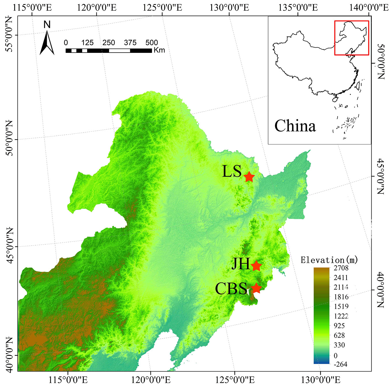
Three large field plots were established in the Changbaishan Nature Reserve (CBS), the Jiaohe Experimental Forest (JH) and the Liangshui Nature Reserve (LS - Fig. 1). The CBS plot is located at 42° 04′ - 42° 23′ N and 127° 55′ - 128° 08′ E. This plot was established in 2014 covering an area of 40 ha (500 × 800 m). The elevation in CBS ranges from 991 to 1046 m. The topography is almost flat, slopes are less than five degrees. The JH plot is located at 43° 57′ - 43° 58′ N, 127° 44′ - 127° 45′ E. The plot was established in 2010 and remeasured in 2015 covering an area of 30 ha (500 × 600 m). The topographic variation is considerable with elevations ranging from 578 to 781 m a.s.l., and a gully between two slopes (facing southeast and southwest). The LS plot is located at 47° 07′ - 47° 14′N, 128° 48′ - 128° 55′ E. The plot was established in 2010 and remeasured in 2015 covering an area of 29.64 ha (380 × 780 m). The topography of the plot is flat with elevations ranging from 380 to 400 m a.s.l.
Fig. 1 - Location of the three large observational study areas in northeastern China. The Changbaishan Nature Reserve (CBS), the Jiaohe Experimental Forest (JH) and the Liangshui Nature Reserve (LS). The map was generated by ArcGIS® ver. 10.3 software (⇒ http://resources.arcgis.com/en/home/). The data is an open access DEM data obtained from the Earth Remote Sensing Data Analysis Center (⇒ https://ssl.jspacesystems.or.jp/ersdac/GDEM/E/).
All woody plants with a diameter at breast height (dbh) ≥ 1 cm were tagged, measured and identified to species. The coordinates of all woody-plant individuals were mapped to the nearest decimeter by steel tape. Altogether 109,338 individual stems were recorded in CBS, 44,583 in JH and 27,879 in the LS plot, belonging to 43, 48 and 32 species, respectively.
Data processing
The CBS data of 2014 and the JH and LS data of 2015 were used in this study. To assess the scale effect on species abundance patterns, we considered four sampling unit sizes, namely 10 × 10 m (0.01 ha), 30 × 30 m (0.09 ha), 60 × 60 m (0.36 ha) and 90 × 90 m (0.81 ha). This particular range of sampling unit size is widely used in studies on forest communities aimed at detecting environmental change of soil and topographical properties as well as spatial aggregation within a local community ([6], [11], [32]). For the calculations at each sampling scale, we divided the area of each plot into a grid of cells. The species abundance was calculated for each cell. The observed species abundances are represented as the mean values of all cells. Tab. 1shows the number of cells, the total area, the number of sampled individuals. Tab. 2presents the variability of species richness, abundance and evenness for each sampling design.
Tab. 1 - General information about the three observational field studies and sampling design used in this analysis.
| Plot | Sampling scale (m×m) |
No. of sampling plots |
Total area (ha) |
No. of individuals |
No. of species |
|---|---|---|---|---|---|
| CBS | 10×10 | 4.000 | 40.00 | 109.338 | 43 |
| 30×30 | 416 | 37.44 | 102.964 | ||
| 60×60 | 104 | 37.44 | 102.964 | ||
| 90×90 | 40 | 32.40 | 90.208 | ||
| JH | 10×10 | 3.000 | 30.00 | 44.583 | 48 |
| 30×30 | 320 | 28.80 | 43.443 | ||
| 60×60 | 80 | 28.80 | 43.443 | ||
| 90×90 | 30 | 24.30 | 36.873 | ||
| LS | 10×10 | 2.964 | 29.64 | 27.879 | 32 |
| 30×30 | 312 | 28.08 | 26.185 | ||
| 60×60 | 78 | 28.08 | 26.185 | ||
| 90×90 | 32 | 25.92 | 24.674 |
Tab. 2 - The variability of species richness, abundance and evenness for each sampling design. (SD): standard deviation.
| Plot | Scale (m×m) |
Richness | Abundance | Evenness | ||||||
|---|---|---|---|---|---|---|---|---|---|---|
| Range | Mean | SD | Range | Mean | SD | Range | Mean | SD | ||
| CBS | 10×10 | 1-16 | 6.85 | 2.21 | 1-95 | 27.42 | 12.07 | 0.26-1.00 | 0.69 | 0.14 |
| 30×30 | 13-25 | 18.57 | 2.42 | 86-468 | 247.50 | 60.51 | 0.21-0.72 | 0.48 | 0.09 | |
| 60×60 | 20-29 | 25.14 | 1.89 | 608-1373 | 990.02 | 167.09 | 0.28-0.62 | 0.41 | 0.06 | |
| 90×90 | 25-33 | 28.65 | 1.79 | 1541-3197 | 2255.2 | 310.52 | 0.28-0.53 | 0.38 | 0.05 | |
| JH | 10×10 | 1-13 | 5.76 | 2.07 | 1-56 | 14.88 | 7.20 | 0.34-1.00 | 0.79 | 0.13 |
| 30×30 | 10-23 | 16.54 | 2.38 | 55-261 | 135.57 | 36.68 | 0.25-0.87 | 0.58 | 0.11 | |
| 60×60 | 18-29 | 23.54 | 2.47 | 298-814 | 542.27 | 106.05 | 0.32-0.69 | 0.50 | 0.08 | |
| 90×90 | 24-33 | 27.97 | 2.70 | 916-1638 | 1227.6 | 194.69 | 0.33-0.61 | 0.45 | 0.07 | |
| LS | 10×10 | 1-13 | 4.70 | 1.77 | 1-45 | 9.46 | 5.09 | 0.50-1.00 | 0.88 | 0.09 |
| 30×30 | 7-21 | 11.72 | 2.03 | 26-198 | 83.93 | 29.77 | 0.40-0.90 | 0.69 | 0.09 | |
| 60×60 | 11-23 | 15.35 | 2.07 | 199-705 | 335.71 | 104.40 | 0.45-0.77 | 0.62 | 0.06 | |
| 90×90 | 14-23 | 18.00 | 1.93 | 483-1255 | 771.06 | 214.31 | 0.48-0.64 | 0.56 | 0.04 | |
Five SAD models that have been widely used in the ecological literature were selected for modeling. Most importantly, these models are all based on specific ecological assumptions which may help to understand certain assembly processes of forest communities. The broken stick ([21]), niche-preemption ([28]) and Zipf ([14]) models are niche based, while the neutral model ([18]) is based on neutral theory. The lognormal model ([30]) was originally thought to be purely statistical resulting from the central limit theorem ([26]). It has been shown, however, to be also associated with niche preemption and population dynamics ([10], [9]). More details about the five models are present in Appendix 1 (Supplementary material).
The chi-square (χ2) statistic at 95% confidence level was used to test the discrepancy of the expected and observed SAD patterns. We used the Bayesian Information Criterion (BIC) to compare the models and to identify the optimum one with the lowest BIC value.
All calculations were carried out in R ver. 3.2.3 ([31]) using the package “vegan” ([29]) and the package “untb” ([17]). The R script that was used to generate the major results is presented in Appendix 2 (Supplementary material).
Results
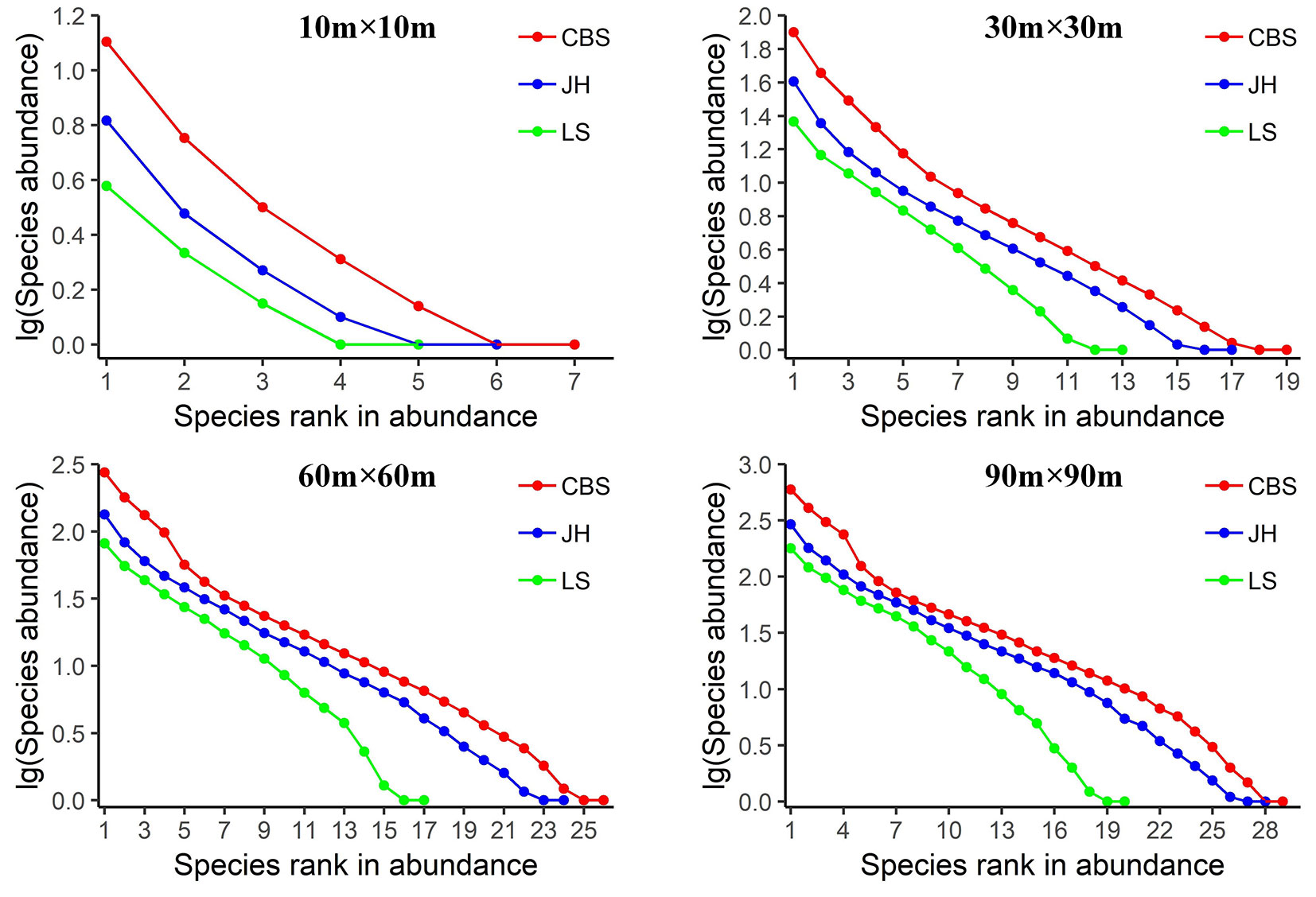
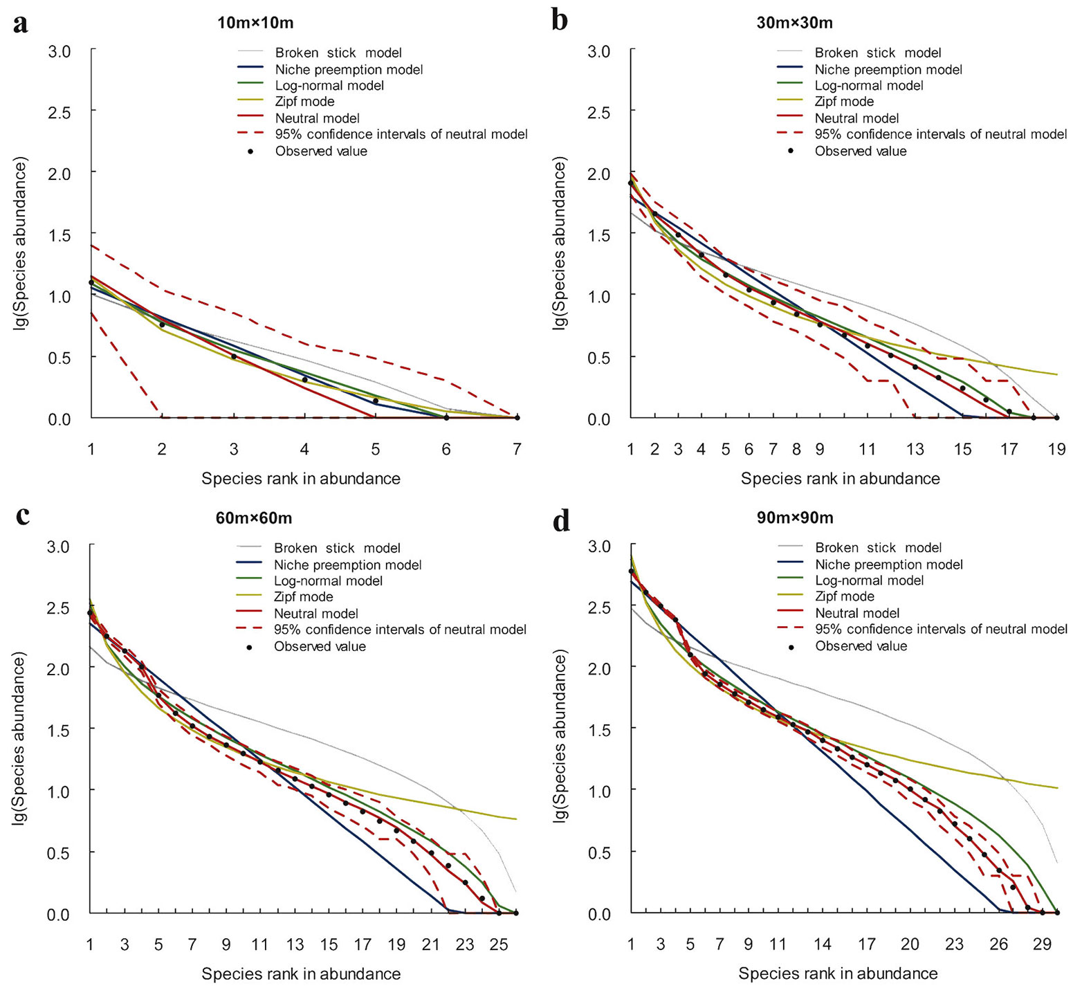
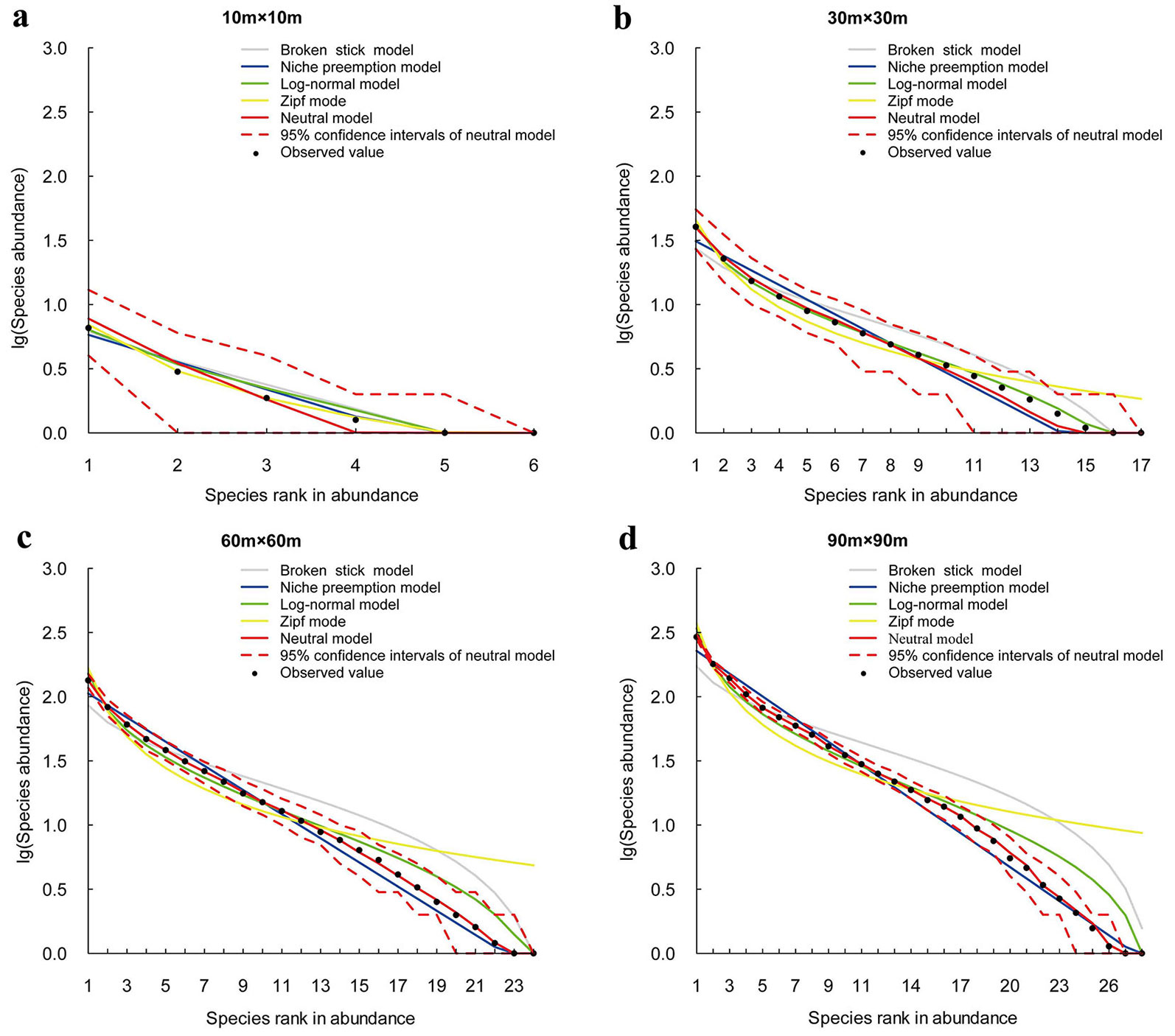
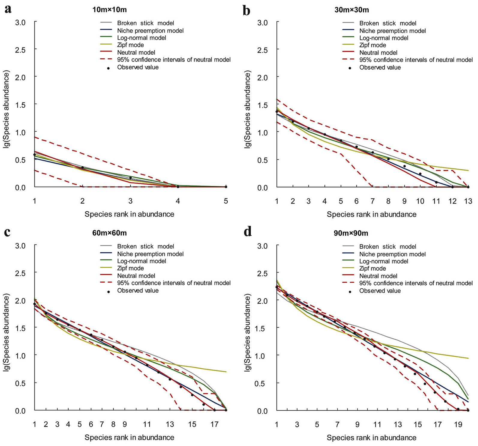
In this study, data of three plots in temperate conifer and broad-leaved mixed forests were analyzed, to check if the sampling effects on SAD pattern are consistent across all localities. For each sampling scale, (i) the general pattern of the SAD (Fig. 2), (ii) the expected SADs for the five candidate models (Fig. 3, Fig. 4, Fig. 5), and (iii) the predictive ability of each SAD model (Tab. 3) are presented. As shown in Fig. 2, the SAD patterns are similar in the three localities, but vary substantially with sample scale. SADs of the smallest sampling scale (10 × 10 m) are characterized by low species richness and high unevenness, with a few common species and some rare species, and a steep decline in the ranked species abundance. As the sample size increases, species richness and evenness are increasing, as well as the number of rare species. The rate of decrease in the ranked species abundance is decreasing. The SADs of the large scales are characterized by high species richness and evenness, with some common species and a large proportion of rare species.
Tab. 3 - Goodness-of-fit test of five models and parameters of the neutral model at four sampling scales. θ is the fundamental diversity index, a parameter of the neutral theory model; m is the immigration rate, a parameter of the neutral theory model. The models were tested at the 95% confidence level, the significant different model were rejected by the test. (**): p < 0.01; (*): 0.01< p < 0.05. (NM): neutral model; (BSM): broken stick model; (NPM): niche preemption model; (LNM): log-normal model; (ZM): Zipf model. CBS, JH and LS refer to Changbaishan, Jiaohe and Liangshui, respectively. (BIC): Bayesian Information Criterion.
| Plot | Sampling scale (m) |
Testing method |
LNM | BSM | ZM | NPM | NM | θ | m |
|---|---|---|---|---|---|---|---|---|---|
| CBS | 10×10 | BIC | -4.71 | 0.90 | -1.95 | -0.53 | 1.37 | 2.73 | 5.1.10-2 |
| χ 2 | 0.17 | 1.64 | 0.24 | 0.56 | 0.97 | ||||
| 30×30 | BIC | 19.14 | 38.84 | 30.48 | 29.26 | -13.56 | 4.63 | 9.4.10-3 | |
| χ 2 | 2.81 | 60.23* | 20.35 | 10.29 | 0.30 | ||||
| 60×60 | BIC | 67.78 | 82.25 | 76.06 | 62.80 | -30.80 | 4.77 | 2.4.10-3 | |
| χ 2 | 34.13 | 430.76** | 200.20** | 51.67** | 0.15 | ||||
| 90×90 | BIC | 104.14 | 119.55 | 112.35 | 96.61 | -29.37 | 4.98 | 1.1.10-3 | |
| χ 2 | 114.21** | 1385.00** | 809.68** | 174.57** | 0.54 | ||||
| JH | 10×10 | BIC | -3.55 | -5.42 | -5.12 | -3.27 | 0.46 | 3.20 | 1.1.10-1 |
| χ 2 | 0.14 | 0.34 | 0.08 | 0.27 | 0.61 | ||||
| 30×30 | BIC | -6.69 | 20.83 | 14.57 | 18.19 | -6.38 | 4.93 | 1.8.10-2 | |
| χ 2 | 0.22 | 10.36 | 8.39 | 4.76 | 0.67 | ||||
| 60×60 | BIC | 38.35 | 54.64 | 52.26 | 44.43 | -23.53 | 4.99 | 4.6.10-3 | |
| χ 2 | 10.28 | 86.70** | 124.92** | 12.13 | 0.12 | ||||
| 90×90 | BIC | 66.12 | 84.21 | 79.96 | 69.82 | -20.11 | 5.00 | 2.0.10-3 | |
| χ 2 | 41.94* | 336.02** | 466.16** | 31.18 | 0.20 | ||||
| LS | 10×10 | BIC | -18.03 | -17.78 | -16.16 | -12.12 | -8.74 | 3.83 | 2.1.10-1 |
| χ 2 | 0.03 | 0.17 | 0.09 | 0.01 | 0.28 | ||||
| 30×30 | BIC | 1.05 | -4.27 | 13.03 | -0.46 | -1.00 | 3.62 | 2.2.10-2 | |
| χ 2 | 0.71 | 0.47 | 6.89 | 0.39 | 0.91 | ||||
| 60×60 | BIC | 29.28 | 24.94 | 36.27 | 13.60 | -13.93 | 3.64 | 5.4.10-3 | |
| χ 2 | 14.29 | 23.05 | 93.49** | 2.44 | 0.08 | ||||
| 90×90 | BIC | 52.33 | 50.33 | 59.21 | 31.25 | -13.63 | 3.86 | 2.5.10-3 | |
| χ 2 | 72.16** | 189.41** | 447.82** | 8.99 | 0.31 |
The predictive ability of the SAD models varies significantly with the sampling scale. The results of chi-square tests and BIC comparison show that, at small sample sizes (10 × 10 m and 30 × 30 m) almost all models show a good fit (Fig. 3, Fig. 4, Fig. 5, Tab. 3). LNM or BSM show the best performance. The observed species abundance distributions thus meet the ecological assumption in all candidate models, but the statistical and niche based models perform better than the neutral model. As sample size increases, more models are rejected since the expected SADs are significantly different from the observed SADs. For example, at the 60 × 60 m scale, the rejected models include BSM, ZM and NPM for Changbaishan, BSM and ZM for Jiaohe, ZM for Linagshui. At the 90 × 90 m scale, the rejected models include BSM, ZM, NPM and LNM for Changbaishan, and BSM, ZM and LNM for both Jiaohe and Liangshui. The rejected models are mostly niche-based, and the number of rejections is increasing with increasing sampling sizes, indicating that the predictive ability of niche models decrease with increasing sampling scale. The results also show that NM is the best model at large sampling sizes (60 × 60 m and 90 × 90 m) in all three localities, indicating that the species abundance distributions can be better explained by the neutral assumption, and the predictive ability of neutral model is increasing with sampling scale.
Discussion
SAD curves change with sample size because the detected diversity patterns are affected by sampling. Species richness increased by about 76%, 79% and 74% towards the largest grain sizes respectively in Changhaishan, Jiaohe and Liangshui. while abundance increased by about 99% in all three localities. Evenness decreased by about 64%, 46% and 56% with increasing grain size, respectively (Tab. 2). The rare species (13, 18 and 11 rare species in Changbaishan, Jiaohe and Liangshui, respectively), mainly includes big canopy trees and small shrubs, such as Deutzia parviflora, Tilia mandshurica, Rosa davurica, Populus davidiana in Changbaishan; Sambucus williamsii, Salix koreensis, Lonicera ruprechtiana, Acer triflorum in Jiaohe; Populus nigra, Rhamnus diamantiaca, Maackia amurensis, Juglans mandshurica in Liangshui, are more likely to be detected in large samples ([23]), which may cause the shape of SAD in rank-abundance plot to become less steep ([27]). Bazzaz ([2]) found a similar result when the temporal scale changed as more species are added with progressive succession. McGill et al. ([27]) found that the SAD curve of species-poor boreal forests is rather flat which could be represented by a geometric model; in contrast, the extreme species-rich tropical forests usually produce SAD curves that follow the neutral model.
In our study, the predictive ability of the niche models decreased with increasing sampling scale, for a series of possible reasons. From a statistical perspective, when the total area of the study plot is fixed, the number of samples at a small grain is greater than that of a large grain. The level of uncertainty associated with parameter estimates increases with decreasing number of samples, i.e., with increasing size of the individual sampling units. When the number of samples is small, outliers carry more weight than if more data are available to buffer their effects ([38]). From the ecological perspective, the attributes of an ecological niche is highly dimensional, and the species response to the environment may be skewed or multimodal ([1]). At small sampling grains, the environment is more homogenous in each sample, and the diversity pattern is mainly dominated by inter-species competition. This may corroborate the niche preemption hypothesis ([2]), which implies that one dominant species may occupy a large fraction of the total niche space, while a second species occupies a similar fraction of the remaining niche space ([28]). With increasing size of sampling units, more heterogeneous environments are included, and the interaction between species and environment becomes more complicated. Such effects may not be well represented by a single-process-based niche model.
The predictive ability of the neutral model increased with increasing sampling scale. The neutral theory predicts that the shape of the local species abundance distribution is a function of the immigration rate ([16]). The immigration rate is likely to be associated with regeneration of new individuals of additional species. In our study, the observed communities are stable with hardly any immigration of new species. Most species in our communities regenerate by seed. As a consequence, the decreasing immigration rate (m) associated with increasing sampling scale, indicates that the spatial turnover of species is greater at small sample unit sizes, and that the intraspecific aggregation is greater at large sample unit sizes. This observation may reflect an increasing effect of a species dispersal limitation ([13]) which suggests that the dispersal mode in our temperate forests (where most broad-leaved trees disperse seeds by wind, conifer trees and shrubs by gravity and animals), may be a key factor in shaping the community pattern at large scales. This observation is consistent with the results of Wang et al. ([36]), who found that in temperate forests in northeastern China, the distribution of trees and shrubs are aggregated because species richness and abundance do not change with sample size in an unbiased way. They concluded that the spatial heterogeneity may be the result of within-community disturbances such as windthrow, fire and insects, which promote the regeneration of a diverse array of species. Green & Plotkin ([16]) also found that the observed left-skewness at larger scales could have resulted from increasing dispersal limitation.
Our findings differ from previous studies which reported that neutral processes are often thought to dominate in species-rich tropical forests. However, in our temperate forests, the number of species found (32 to 48 on 20 to 40 ha - Tab. 1) is more limited, and neutral models show nevertheless a good fit at almost all scales. It is possible that this unexpected result originates from over-fitting of the neutral models. The format of the neutral model possesses the ability to fit many observed patterns with smooth curves. In some situations, the better fit of a neutral model may be the result of a greater flexibility compared to other models without necessarily implying a dominance of neutral processes. We assume that the neutral model which showed better performance at large sampling scales, may reveal underlying processes, such as the aforementioned dispersal limitation, that generated a particular pattern. Foster & Warton ([13]) found that the better fit of a neutral model may indicate particular plant communities at similar environmental conditions are composed of neutrally-interacting species.
When comparing the relative accuracy of different models across sampling scales, we found that model performance depends on the scale. Niche-based models gave a better fit at small scales while the neutral model performed better at large scales. This result is consistent with Gao et al. ([15]) who reported that, in temperate forests, dominance of species with positive effects on diversity at small scales (0-10 m) supports niche theory, that species diversity is improved by variation in niche utilization. Dominance of neutral species, i.e., species with no significant effects on diversity, at large scales (10-50 m) supported the assumption that community diversity was a result of a neutral process. These findings suggest that both niche and neutral processes are important in structuring a community. Actually, the connection between neutral or niche distribution is not completely exclusive ([9]). For example, broken stick model ([21]) is usually interpreted as niche-based when viewed as a sequential breakage model, but may just as well be regarded as neutral when viewed as a stochastic simultaneous breakage model ([34], [33]). Such results imply that interpretations based on a single pattern should be interpreted with caution. To accurately predict SAD’s of similar ecosystems, observations in large plots and across sampling scales are required.
Conclusions
Based on observations from three large field plots with mapped trees in the temperate forests in northeastern China, five different SAD models were used to examine how expected SADs differ from observed ones across four sampling scales. The results show strong effects of sampling scales on SAD. The primary results are: (i) the shape of the species abundance distribution varies with the sampling scale; (ii) the predictive ability of the niche-based model decreased with increasing sampling scale; (iii) the predictive ability of the neutral model increased with increasing sampling scale; (iv) the niche-based models provided a better fit at the small sampling scales, while the neutral model gave a better fit at the large sampling scales. The fact that only three (though very large) localities were included limits the general validity of our findings. We conclude that there is no inherently superior model representing the SADs, and recommend that in future studies the scale effects in SAD modeling should be given greater attention.
Acknowledgements
This research is supported by the Key Project of National Key Research and Development Plan (2017YFC0504005) and the Program of National Natural Science Foundation of China (31670643). This paper has benefitted from the valuable suggestions of two anonymous reviewers.
References
CrossRef | Gscholar
Gscholar
CrossRef | Gscholar
Gscholar
CrossRef | Gscholar
Gscholar
Authors’ Info
Authors’ Affiliation
Peng Zhang 0000-0002-6769-3310
Xiuhai Zhao 0000-0003-0879-4063
Chunyu Fan 0000-0002-3360-2919
Chunyu Zhang 0000-0003-3091-5060
Research Center of Forest Management Engineering of State Forestry and Grassland Administration, Beijing Forestry University, 100083 Beijing (China)
College of Forestry, Northwest A&F University, Yangling, Shanxi 712100 (China)
Faculty of Forestry and Forest Ecology, Georg-August-University Göttingen, Büsgenweg 5, D-37077 Göttingen (Germany)
Department of Forest and Wood Science, University of Stellenbosch (South Africa)
Corresponding author
Paper Info
Citation
Tan L, Zhang P, Zhao X, Fan C, Zhang C, Yan Y, Von Gadow K (2020). Analysing species abundance distribution patterns across sampling scales in three natural forests in Northeastern China. iForest 13: 482-489. - doi: 10.3832/ifor3211-013
Academic Editor
Michele Carbognani
Paper history
Received: Aug 07, 2019
Accepted: Aug 15, 2020
First online: Nov 01, 2020
Publication Date: Dec 31, 2020
Publication Time: 2.60 months
Copyright Information
© SISEF - The Italian Society of Silviculture and Forest Ecology 2020
Open Access
This article is distributed under the terms of the Creative Commons Attribution-Non Commercial 4.0 International (https://creativecommons.org/licenses/by-nc/4.0/), which permits unrestricted use, distribution, and reproduction in any medium, provided you give appropriate credit to the original author(s) and the source, provide a link to the Creative Commons license, and indicate if changes were made.
Web Metrics
Breakdown by View Type
Article Usage
Total Article Views: 39935
(from publication date up to now)
Breakdown by View Type
HTML Page Views: 33848
Abstract Page Views: 2637
PDF Downloads: 2701
Citation/Reference Downloads: 10
XML Downloads: 739
Web Metrics
Days since publication: 2007
Overall contacts: 39935
Avg. contacts per week: 139.29
Article Citations
Article citations are based on data periodically collected from the Clarivate Web of Science web site
(last update: Mar 2025)
Total number of cites (since 2020): 6
Average cites per year: 1.00
Publication Metrics
by Dimensions ©
Articles citing this article
List of the papers citing this article based on CrossRef Cited-by.
Related Contents
iForest Similar Articles
Research Articles
Distribution factors of the epiphytic lichen Lobaria pulmonaria (L.) Hoffm. at local and regional spatial scales in the Caucasus: combining species distribution modelling and ecological niche theory
vol. 17, pp. 120-131 (online: 30 April 2024)
Research Articles
Quantifying forest net primary production: combining eddy flux, inventory and metabolic theory
vol. 10, pp. 475-482 (online: 12 April 2017)
Research Articles
Predicting the effect of climate change on tree species abundance and distribution at a regional scale
vol. 1, pp. 132-139 (online: 27 August 2008)
Research Articles
Effect of imperfect detection on the estimation of niche overlap between two forest dormice
vol. 11, pp. 482-490 (online: 18 July 2018)
Research Articles
Effects of functional traits on the spatial distribution and hyperdominance of tree species in the Cerrado biome
vol. 15, pp. 339-348 (online: 01 September 2022)
Research Articles
Local ecological niche modelling to provide suitability maps for 27 forest tree species in edge conditions
vol. 13, pp. 230-237 (online: 19 June 2020)
Research Articles
Single-tree influence on understorey vegetation in five Chinese subtropical forests
vol. 5, pp. 179-187 (online: 02 August 2012)
Research Articles
Former charcoal platforms in Mediterranean forest areas: a hostile microhabitat for the recolonization by woody species
vol. 10, pp. 136-144 (online: 06 October 2016)
Research Articles
Light availability influences the invasion of Teline monspessulana (L.) K. Koch in a temperate fragmented forest in Central Chile
vol. 15, pp. 411-416 (online: 19 October 2022)
Research Articles
Scale dependency of the effects of landscape structure and stand age on species richness and aboveground biomass of tropical dry forests
vol. 16, pp. 234-242 (online: 23 August 2023)
iForest Database Search
Search By Author
Search By Keyword
Google Scholar Search
Citing Articles
Search By Author
Search By Keywords
PubMed Search
Search By Author
Search By Keyword

