Contribution of environmental variability and ecosystem functional changes to interannual variability of carbon and water fluxes in a subtropical coniferous plantation
iForest - Biogeosciences and Forestry, Volume 9, Issue 3, Pages 452-460 (2016)
doi: https://doi.org/10.3832/ifor1691-008
Published: Jan 25, 2016 - Copyright © 2016 SISEF
Research Articles
Abstract
Accurate quantification of the contribution of environmental variability and functional changes to the interannual variability of net ecosystem production (NEP) and evapotranspiration (ET) in coniferous forests is needed to understand global carbon and water cycling. This study quantified these contributions to the interannual variability of NEP and ET for a subtropical coniferous plantation in southeastern China, and the effect of drought stress on these contributions was also investigated. NEP and ET were derived from eddy covariance measurements carried out over the period 2003-2012. A homogeneity-of-slopes model was adopted to quantify the contribution to the interannual variability of these fluxes. Environmental variability accounted for 71% and 85.7% of the interannual variability of NEP and ET, respectively; however, functional changes accounted for only 11.3% and 5.9%, respectively. Furthermore, functional changes explained more of the interannual variability of NEP in dry years (16.3%) than in wet years (3.8%), but there was no obvious change in the contribution of functional changes to the interannual variability of ET in dry (4.7%) or wet (5.5%) years. Thus, environmental variability rather than ecosystem functional changes dominated the interannual variability of both ET and NEP. However, different environmental variables controlled the interannual variability of NEP and ET. The results also indicated that, compared with NEP, ET was more resistant to drought stress through the self-regulating mechanisms of this plantation.
Keywords
Environmental Variability, Functional Changes, Net Ecosystem Production (NEP), Evapotranspiration (ET), Subtropical Plantation
Introduction
Understanding what drives the interannual variability of carbon and water fluxes is needed to predict global carbon and water cycling and can also provide a basis for improving models of carbon and water processes ([1], [14]). Numerous studies showed that the interannual variability of carbon and water fluxes is controlled by both environmental variability and ecosystem functional changes ([36], [43]). Until recently, models estimating ecosystem carbon and water fluxes were mainly based on the controlling effect of environmental variability ([10], [5], [18]). However, a discrepancy has generally been reported between the observed carbon or water fluxes and those estimated from models based on environmentally controlled mechanisms ([11], [31], [15]). Functional changes include changes in ecosystem structure and vegetation physiological processes ([20]), and they can be quantified as the indirect effect of environmental variability on biological and ecological processes that regulate the interannual variability of forest carbon or water fluxes ([20], [31]). Models that consider both environmental controls and functional changes provide more accurate simulations than those considering only environmental controls ([37]).
Coniferous forests account for 36% of all forested areas globally ([7]), and thus functional changes in coniferous forests at a regional scale may influence carbon and water cycles at a global scale ([11], [5]). Previous studies suggested that environmental variability dominated the interannual variability of net ecosystem production (NEP - [11]) or evapotranspiration (ET - [41]) in coniferous forests. However, some studies found that functional changes explain the interannual variability of NEP in a temperate pine forest ([24]) and the ET in a subtropical pine forest ([2]). Furthermore, Yu et al. ([39]) and Keenan et al. ([16]) reported that carbon and water fluxes were both mainly regulated by the opening of leaf stomata of the vegetation. However, few studies have investigated the importance of environmental variability and functional changes on the interannual variability of NEP and ET in coniferous forests ([22]).
Drought stress is considered a critical climate event that influences ecosystem carbon and water cycles ([3], [19]). Zha et al. ([41]) found that under drought conditions functional changes or self-regulating mechanisms of the vegetation determine the interannual variability of ET in a coniferous forest. Drought frequency may increase in mid- and high-latitude regions as uneven precipitation distribution will increase with climate change ([12]). An analysis of the controlling effect of environmental variability and functional changes on the interannual variability of NEP and ET in coniferous forests, especially in response to drought stress, is needed to predict the effects of climate change on carbon and water cycles at regional and global scales ([1]).
Southern China has the largest global evergreen subtropical forest covering 53 million ha, and coniferous plantations account for nearly half of this total forest area ([32]). This region is characterized by a subtropical humid monsoon climate with abundant water and energy resources; however, drought stress may occur during summer and autumn because high temperatures and precipitation in southeastern China do not always coincide, which is associated with a Pacific subtropical high pressure system ([34], [29]).
In this study the homogeneity-of-slopes (HOS) model developed by Hui et al. ([11]) was applied to eddy covariance measurements taken over the period 2003-2012 in a subtropical coniferous plantation in southeastern China. The objectives of this study were to: (i) quantify the contribution of environmental variability and functional changes to the interannual variability of NEP and ET; and (ii) investigate whether the contribution of these factors changes under drought conditions.
Methods
Site description
The Qianyanzhou flux observation site (26° 44′ 52″ N, 115° 03′ 47″ E; elevation: 102 m a.s.l.), a member of ChinaFLUX, is located at the Qianyanzhou station of Chinese Ecosystem Research Network (CERN) in southeastern China. The total experimental area occupies 212.13 ha. This area is influenced by a subtropical monsoon climate, with mean annual temperature and precipitation of 17.9 °C and 1472.8 mm, respectively, according to meteorological records for 1985-2012. The soil is red earth, predominantly weathered from red sandstone, and is classified as a Typic Dystrudept in United States soil taxonomy. The soil bulk density at the surface (0-40 cm) is 1.57 g cm-3 ([28]).
The flux tower is located in the foothills, with a slope within the range of 2.8-13.5°. The evergreen coniferous plantation was planted in 1985. The mean heights of Masson pine (Pinus massoniana L.), Chinese fir (Cunninghamia lanceolata L.) and slash pine (P. elliottii E.) were 11.2, 11.8, and 14.3 m, respectively, and the corresponding mean stem densities were 700, 93, and 545 stems ha-1; mean diameters at breast height were 13.6, 13.8, and 18.2 cm, respectively, according to a survey of vegetation surrounding the flux tower carried out in 2008. The dominant shrub was Loropetalum chinense, and the dominant herbaceous species were Arundinella setosa and Helicteres angustifolia ([17]). Further information on the site are reported by Wen et al. ([34]).
Eddy covariance and environmental variable measurements
The eddy covariance instruments were mounted 39.6-m high on a tower in 2002. The concentrations of carbon dioxide and water vapor were measured using an LI-7500 open-path CO2/H2O analyzer (Li-7500, Li-Cor Inc., Lincoln, NE, USA), and three-dimensional wind speed and virtual temperature were detected using a three-dimensional sonic anemometer (CSAT3, Campbell Scientific Inc., Logan, UT, USA). All raw flux data were sampled at 10 Hz, and the 30-min mean fluxes were logged and stored by a CR5000 datalogger (CR5000, Campbell Scientific Inc., USA).
Auxiliary environmental variables were also measured. A pyranometer (CM11, Kipp & Zonen Inc., Delft, the Netherlands), a quantum sensor of photosynthetic active radiation (LI190SB, Li-Cor Inc., USA), and a four-component net radiometer (CNR-1, Kipp & Zonen Inc., the Netherlands) were used to measure the radiation. The vertical profiles of air temperature (Ta) and relative humidity (HMP45C, Campbell Scientific Inc., USA), as well as wind speed (A100R, Vector Inc., Denbighshire, UK), were measured at seven levels (1.6, 7.6, 11.6, 15.6, 23.6, 31.6, and 39.6 m above the ground). The vertical profiles of soil temperature (2, 5, 20, 50, and 100 cm below the ground) and soil water content (SWC - 5, 20, and 50 cm below the ground) were measured with thermocouples (105T and 107-L, Campbell Scientific Inc., USA) and TDR probes (CS615-L, Campbell Scientific Inc., USA), respectively. Soil heat flux was measured through two plates (HFT-3, Campbell Scientific Inc., USA) placed at a depth of 5 cm below ground surface. Precipitation was monitored using a rain gauge (52203, RM Young Inc., Traverse City, MI, USA). All the above environmental variables were sampled at 1 Hz and stored at 30-min averages by dataloggers (CR10XTD, Campbell Scientific Inc., USA).
Processing of eddy covariance and environmental variables
Planar fit rotation can reduce the run-to-run stress errors caused by sampling effects, and enable an unbiased estimate of the lateral stress ([35]). Thus, for the 30-min mean fluxes, planar fit rotation was applied to the wind components to remove the effect of instrument tilt or irregularity of the air flow at monthly intervals ([34]). The Webb-Pearman-Leuning correction was performed to adjust density changes resulting from fluctuations in heat and water vapor ([33]). Anomalous or spurious flux values caused by precipitation, system failure and power interruption were screened and eliminated. Any flux value that exceeded five times the standard deviation (SD) within a window of 10 values was discarded. Flux value and environmental data were broadly divided into daytime and nighttime according to the solar elevation angle. To avoid a possible underestimation of the fluxes under stable conditions during the night (solar elevation angle < 0°), the effect of friction velocity was identified for each year according to the method of Reichstein et al. ([23]). The carbon and water fluxes at night were excluded when the value of the friction velocity was < 0.19 m s-1, which was the maximum friction velocity threshold during 2003-2012 ([28]). Thus, data gaps were produced. During 2003-2012, the average daytime and nighttime reliable data coverage was 75% and 21% for NEP, respectively, and correspondingly 80% and 25% for ET. In addition, due to system failure and power interruption, the average data gaps for all auxiliary environmental data mentioned above for nighttime (2%) were nearly three times as frequent as those for daytime (0.7%) over the period 2003-2012.
Because the majority of nighttime fluxes were unavailable, and missing fluxes had to be estimated based on environmental variables, some autocorrelation between environmental variables and estimated nighttime fluxes was inevitable ([9]). Thus, to avoid this autocorrelation effect, only the available daytime NEP and ET were analyzed. Half-hour mean daytime values for NEP, ET, and the corresponding environmental factors were summarized into daily averages, which were transformed from non-linear relationships between the instantaneous half-hour mean fluxes and environmental variables into linear functions for the regression analysis ([11]). To minimize fluctuations in daily values, weekly mean values were computed ([21], [31]). Daily values were calculated based on >16 available half-hour daytime data, and weekly values were calculated based on > 4 available daily data.
HOS model
A HOS model developed by Hui et al. ([11]) was used in this study to quantify the contribution of seasonal environmental variability, interannual environmental variability, and functional changes to the interannual variability of NEP and ET. To estimate the effects of seasonal and interannual environmental variability on the interannual variability of NEP and ET, annual cycles of NEP and ET must be considered. The comparison of fluxes in a given year with the values at a similar point in the annual cycle in other years gives a measure of temporal variability within an ecosystem ([11], [20], [31]). Any significant change (p<0.05) in the slope of the regression between NEP or ET and a given environmental variable among different years is usually assumed to indicate an indirect effect of an environmental variable. In the HOS model, the assemblage of all indirect effects of environmental variables on NEP or ET can be interpreted through an altered biotic response, and can be referred to as “functional changes” ([11]).
If the year-to-year response of NEP or ET to environmental variables does not involve functional changes, the slope describing the relationship between the environmental variable and NEP or ET will not vary throughout the year, and the controlling mechanism of environmental variables can be calculated using a simple regression (eqn. 1):
otherwise, the controlling mechanism of environmental variables can be calculated using the HOS model (eqn. 2):
In the above equations, i is the i-th year (i=1, 2,…, y, y=10 in this study), j is the j-th week of the year, k is the k-th environmental variable, Yij is the observed NEP or ET, and Xijk is an environmental variable measured at the j-th week of the i-th year for the k-th environmental variable. Additionally, the term bik is the slope that links the interactive terms of year and k-th environmental variable with the NEP or ET, and eij is the random error term associated with observed Yij.
As outlined by Hui et al. ([11]), when there is one or more years of environmental variable interactions with NEP or ET, the sum of the squares of the total deviation of all observed and modeled NEP or ET (SST) can be explained by functional changes (SSf), random error (SSe), interannual environmental variability (SSi), and seasonal environmental variability (SSs) as follows (eqn. 3, eqn. 4, eqn. 5, eqn. 6, eqn. 7):
In these equations, Yij and Yij’ are the estimated NEP or ET using eqn. 1 and eqn. 2, respectively. The SSf can represent the contribution of functional changes (indirect effects of environmental variables) to the interannual variability of fluxes. Mathematically, the flux estimated from eqn. 1 (Yij) can expand to linear components as (eqn. 8):
where Y.j is the mean of the estimated NEP or ET across all the years on the j-th week, Y is the mean of the estimated NEP or ET from eqn. 1, and Yij is the mean of all observed values for NEP or ET. The terms (Yij - Y.j) and (Y.j - Y) represent the interannual and seasonal environmental variability deviations, respectively. Thus, SSi and SSs were calculated to represent the contribution of interannual and seasonal environmental variability to interannual variability of fluxes, respectively. Further details regarding the procedure of the HOS model can be found in Hui et al. ([11]) and Polley et al. ([20]).
In this study, environmental variables such as photosynthetic photon flux density (PPFD), Ta, SWC, and vapor pressure deficit (VPD) were selected as predictors for the interannual variability of NEP. Net radiation (Rn), Ta, SWC, and VPD were selected as predictors for the interannual variability of ET. The results indicated that all these environmental variables were linearly correlated with NEP or ET, respectively. To consider the correlations among these environmental variables ([11]), we first used a multiple linear regression analysis (stepwise method) to identify the environmental variables that significantly controlled the weekly means of daytime NEP or ET (α = 0.05). Then, significant differences in slopes between NEP or ET and the environmental variable that were retained in the final multiple regression models among the years were assessed using an F-test through multivariate analysis in SPSS (Version 16.0, Chicago, IL, USA). If there were any significant differences (p<0.05) in slopes, the HOS model was used. Finally, the contribution of seasonal environmental variability, interannual environmental variability, and functional changes to the interannual variability of NEP or ET were quantified using eqn. 3-7.
Budyko’s Aridity Index
Budyko’s aridity index is the ratio of the precipitation amount to potential evapotranspiration ([4]). An index value < 1 means that the ecosystem is water limited, and this criterion has been used to detect periods of drought stress in coniferous forest and grassland ecosystems ([26], [29]).
Results
Seasonal and interannual variability of environmental variables
The seasonal variability of Rn, PPFD, Ta, and VPD exhibited single peaks, with the maximum and minimum values occurring in summer (June-August) and winter (December-February), respectively (Fig. 1). At the same time, the seasonal variability of SWC at depths of 5 cm, 20 cm, and 50 cm (SWC5cm, SWC20cm, and SWC50cm, respectively) was closely related to precipitation, with higher values in the first half and lower values in the second half of the year (Fig. 1c). This high temperature and lack of sufficient precipitation in summer and autumn may have resulted in seasonal drought stress for this coniferous plantation. The monthly mean values for Budyko’s aridity index in July, October, and November in 2003, 2007, and 2010 were < 1, indicating that the ecosystem was water limited (Fig. 1d). Thus, we defined these three years as dry years and the remaining years as wet years based on the seasonal variability of Budyko’s aridity index.
Fig. 1 - Seasonal and interannual variability of monthly daytime environmental variables during 2003-2012. (a) net radiation (Rn) and photosynthetic photon flux density (PPFD), (b) air temperature (Ta) and vapor pressure deficit (VPD), (c) soil water contents at depths of 5, 20 and 50 cm (SWC5cm, SWC20cm and SWC50cm, respectively), and (d) Budyko’s aridity index.
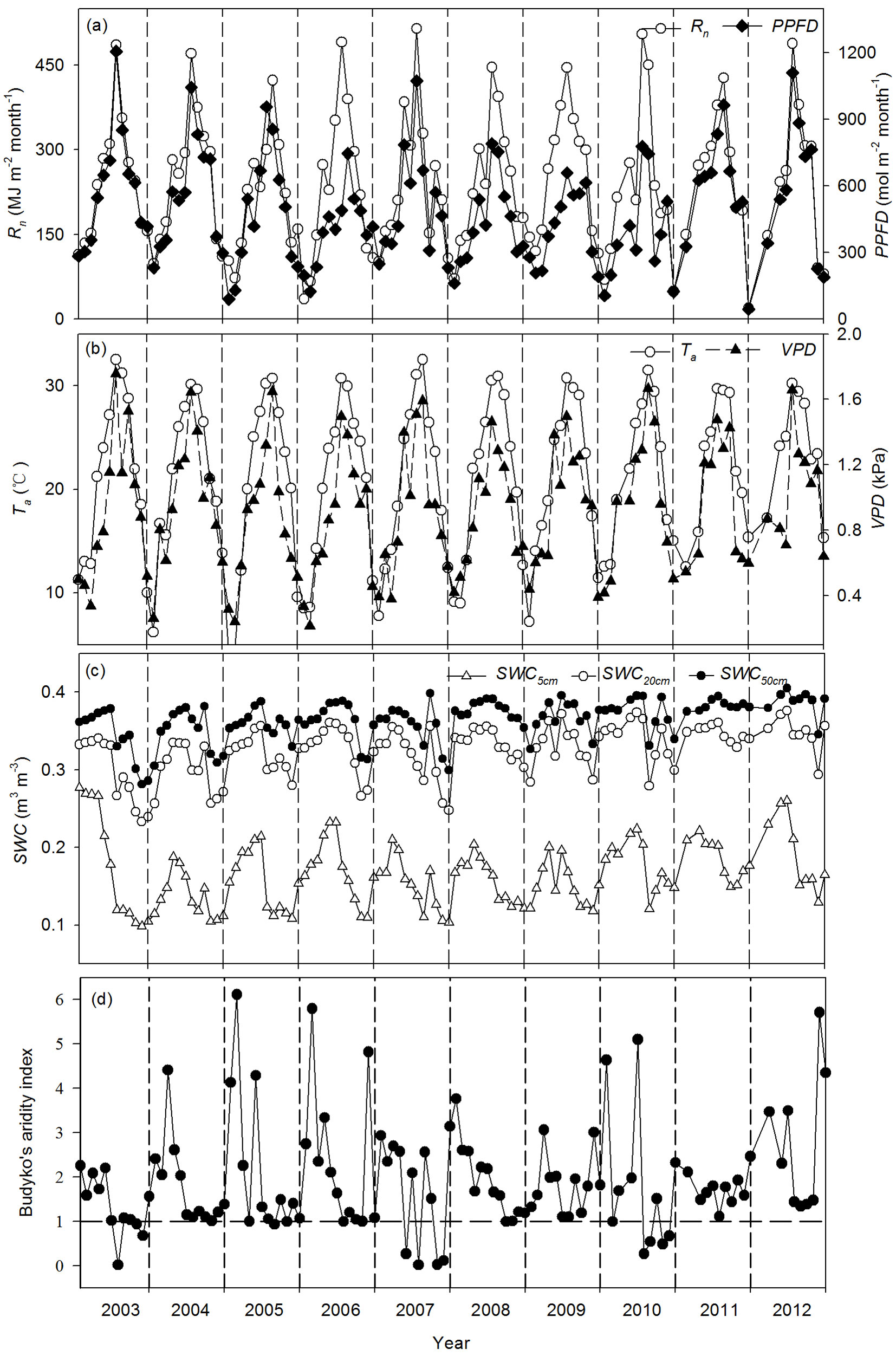
Annual environmental variables differed among the years. The annual sums of Rn ranged from 2627.3 MJ m-2 (2005) to 3070.3 MJ m-2 (2009). The maximum and minimum annual mean values for daytime Ta was 24.2 °C (2012) and 20.9 °C (2006), respectively. The average annual daytime VPD ranged from 1.07 kPa (2003) to 0.86 kPa (2006). The maximum annual mean values for daytime SWC5cm and SWC50cm were both observed in 2012 and were 0.20 m3 m-3 and 0.39 m3 m-3, respectively. The minimum annual mean values for daytime SWC5cm and SWC50cm were 0.14 m3 m-3 (2004) and 0.34 m3 m-3 (2003), respectively.
Seasonal and interannual variability of NEP and ET
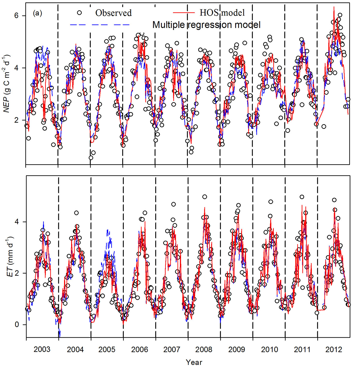
Weekly means of daytime NEP and ET varied seasonally and interannually during 2003-2012 (Fig. 2). Generally, NEP and ET increased from a lower winter value to a maximum during summer. However, NEP and ET declined during summer and autumn droughts in 2003, 2007, and 2010 (Fig. 2). During dry years, the decrease in magnitude of ET was smaller than that of NEP. For example, in 2003, daytime NEP dropped by 63.8% (from 4.7 g C m-2 d-1 to 1.7 g C m-2 d-1), while daytime ET dropped by 59.5% (from 3.7 mm d-1 to 1.5 mm d-1) during summer drought. The average (± SD) annual daytime NEP was 896.9 ± 46.3 g C m-2, with a range of 818.9 g C m-2 (2003) to 964.9 g C m-2 (2012). Meanwhile, the average annual daytime ET was 526.7 ± 73.8 mm, with a range of 364.2 mm (2005) to 624.6 mm (2009). The obviously lower daytime ET for all of 2005 was attributed mainly to the lower Rn in this year ([34]).
Fig. 2 - Seasonal and interannual variability of weekly means of daytime carbon and water fluxes during 2003-2012. (a) net ecosystem production (NEP) and (b) evapotranspiration (ET). Dashed lines indicate flux estimated from a multiple regression model, and solid lines indicate flux estimated from a homogeneity-of-slope (HOS) model.
Regulation of environment variability and functional changes on the interannual variability of NEP and ET during 2003-2012
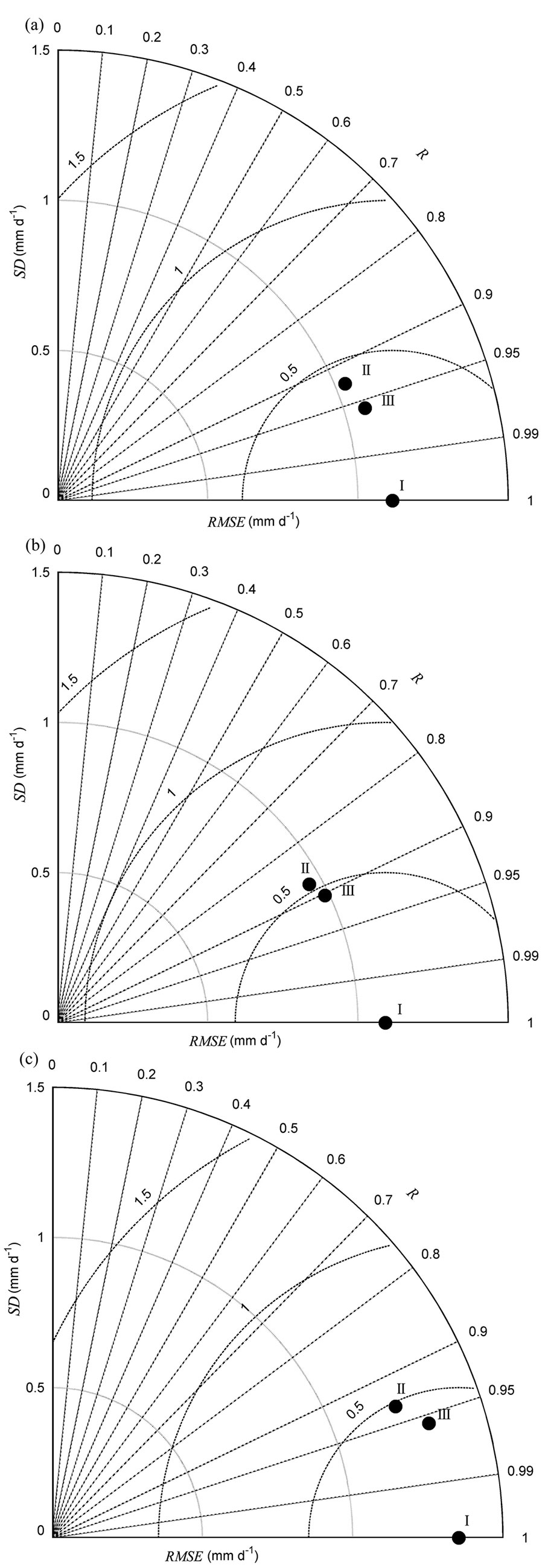
There were differences in the seasonal variability of NEP estimated from multiple regression and HOS models (Fig. 2a). A synthetic comparison of observed and modeled NEP was analyzed through the Taylor’s diagram method (Fig. 3a).
Fig. 3 - Taylor’s diagrams summarizing the performance of modeled net ecosystem production (NEP) compared with observed NEP. (a) during 2003-2012, (b) in dry years (NEP_dry), and (c) in wet years (NEP_wet). “I” indicates observed flux, “II” indicates multiple regression modeled flux, and “III” indicates homogeneity-of-slope (HOS) model fitted flux. R is the correlation coefficient, SD is the standard deviation, and RMSE is the root mean square error between observed and modeled fluxes. See Taylor ([30]) for further Taylor’s diagram details.
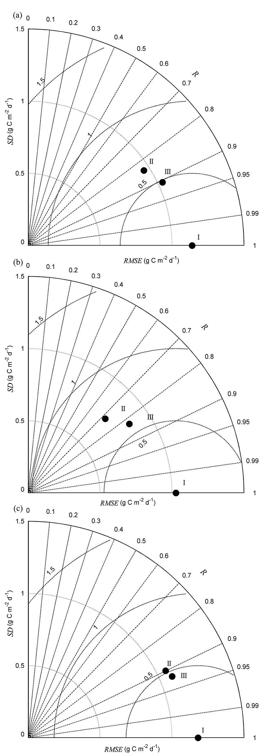
The multiple regression was used to detect environmental variables that significantly controlled the interannual variability of NEP. The final stepwise multiple regression analysis showed that SWC5cm, VPD, Ta, and PPFD significantly influenced NEP (Tab. 1). The F-test showed that the slopes between NEP and some environmental variables (i.e., VPD and SWC5cm) varied significantly among years (p<0.001 - Tab. 2). Thus, a HOS model could be used. The HOS model improved the NEP estimation, compared with the multiple regression model, with coefficients of determination of 0.82 and 0.71, respectively. The HOS modeled values tracked the declining NEP in the summers of 2003, 2007, and 2010 and the obviously higher NEP for all of 2012 (Fig. 2a). Based on the synthetic comparison of correlation (R), SD, and root mean square error (RMSE) between the modeled and observed NEP in a Taylor’s diagram (Fig. 3a), the NEP estimated from the HOS model matched the observed NEP better than the multiple regression model.
Tab. 1 - The final stepwise multiple regression model for weekly means of daytime net ecosystem production (NEP) and evapotranspiration (ET) during 2003-2012, in dry years (NEP_dry and ET_dry), and in wet years (NEP_wet and ET_wet), respectively, at the Qianyanzhou site. (PPFD): photosynthetic photon flux density (mol m-2); (Ta): air temperature (°C); (VPD): vapor pressure deficit (kPa); (SWC5cm): soil water content at depth of 5 cm (m3 m-3); (SWC50cm): soil water content at depth of 50 cm (m3 m -3); (Rn): net radiation (MJ m-2).
| Equations | R2 | P |
|---|---|---|
| NEP = 4.27 SWC5cm - 0.55 VPD + 0.13 Ta + 0.07 PPFD - 0.63 | 0.71 | <0.001 |
| NEP_dry = -1.36 VPD + 0.13 Ta + 0.05 PPFD + 0.54 | 0.52 | <0.001 |
| NEP_wet = 4.43 SWC5cm + 0.11 Ta + 0.06 PPFD - 0.75 | 0.80 | <0.001 |
| ET = 7.52 SWC50cm + 0.57 VPD + 0.15 Rn + 0.07 Ta - 3.52 | 0.86 | <0.001 |
| ET_dry = 9.34 SWC50cm + 0.72 VPD + 0.07 Ta - 3.61 | 0.77 | <0.001 |
| ET_wet = 6.16 SWC50cm + 0.60 VPD + 0.14 Rn + 0.04 Ta - 3.13 | 0.86 | <0.001 |
Tab. 2 - The F-test of the homogeneity-of-slope (HOS) model for weekly means of daytime net ecosystem production (NEP) during 2003-2012, in dry years (NEP_dry), and in wet years (NEP_wet), respectively, at the Qianyanzhou site. (PPFD): photosynthetic photon flux density (mol m-2); (Ta): air temperature (°C); (VPD): vapor pressure deficit (kPa); (SWC5cm): soil water content at depth of 5 cm (m3 m-3); HOS model: NEP ~(VPD + SWC5cm + Ta + PPFD) + (VPD + SWC5cm) × year; NEP_dry ~(Ta + VPD + PPFD) + (VPD) × year; NEP_wet ~(Ta + SWC5cm + PPFD) + (Ta) × year.
| Parameter | Source | Variable | MS | F | p |
|---|---|---|---|---|---|
| NEP | Environmental variability | VPD | 13.1 | 58.1 | <0.001 |
| SWC 5cm | 6.0 | 26.4 | <0.001 | ||
| T a | 87.0 | 385.1 | <0.001 | ||
| PPFD | 45.4 | 201 | <0.001 | ||
| Functional changes | VPD×Year | 2.8 | 12.5 | <0.001 | |
| SWC5cm×Year | 1.1 | 5.1 | <0.001 | ||
| Error | - | 0.23 | - | - | |
| NEP_dry | Environmental variability | T a | 53.9 | 153.1 | <0.001 |
| VPD | 9.4 | 27.3 | <0.001 | ||
| PPFD | 21.7 | 63.2 | <0.001 | ||
| Functional changes | VPD×Year | 3.2 | 9.3 | <0.001 | |
| Error | - | 0.3 | - | - | |
| NEP_wet | Environmental variability | T a | 59.8 | 274 | <0.001 |
| SWC 5cm | 4.5 | 20.4 | <0.001 | ||
| PPFD | 28.5 | 130.5 | <0.001 | ||
| Functional changes | Ta×Year | 0.7 | 3.3 | =0.004 | |
| Error | - | 0.2 | - | - |
The seasonal variability of ET estimated from the multiple regression and HOS models also showed differences (Fig. 2b). The final multiple regression model for ET contained four environmental variables: SWC50cm, VPD, Rn, and Ta (Tab. 1). The F-test showed that the slopes between ET and certain environmental variables (SWC50cm and VPD) varied significantly among the years (p<0.001 - Tab. 3). The HOS model also tracked declining ET in the summers of 2003, 2007, and 2010, as well as the obviously lower ET for all of 2005 (Fig. 2b). The coefficients of determination between the observed and modeled ET increased from 0.86 for the multiple regression model to 0.92 for the HOS model. The synthetic comparison in the Taylor diagram (Fig. 4a) showed that ET estimated from the HOS model matched observed ET better than that estimated from the multiple regression model.
Tab. 3 - The F-test of the homogeneity-of-slope (HOS) model for weekly means of daytime evapotranspiration (ET) during 2003-2012, in dry years (ET_dry), and in wet years (ET_wet), respectively, at the Qianyanzhou site. (Rn): net radiation (MJ m-2); (Ta): air temperature (°C); (VPD): vapor pressure deficit (kPa); (SWC50cm): soil water content at depth of 50 cm (m3 m-3); HOS model: ET~(Rn+Ta +VPD+SWC50cm) + (VPD+SWC50cm) × year; ET_dry~(Ta +VPD+SWC50cm) + (VPD+SWC50cm)×year; ET_wet~(Rn+Ta +VPD+SWC50cm) + (Ta) × year.
| Parameter | Source | Variable | MS | F | p |
|---|---|---|---|---|---|
| ET | Environmental variability | R n | 14.1 | 129.4 | <0.001 |
| T a | 2.7 | 24.7 | <0.001 | ||
| VPD | 5.7 | 52.5 | <0.001 | ||
| SWC 50cm | 7.8 | 71.6 | <0.001 | ||
| Functional changes | VPD×Year | 1.6 | 14.5 | <0.001 | |
| SWC50cm×Year | 0.3 | 3.2 | <0.001 | ||
| Error | - | 0.1 | - | - | |
| ET_dry | Environmental variability | T a | 5.3 | 23 | <0.001 |
| VPD | 8 | 34.6 | <0.001 | ||
| SWC 50cm | 8.1 | 34.8 | <0.001 | ||
| Functional changes | VPD×Year | 2.8 | 12.1 | <0.001 | |
| SWC50cm×Year | 1.7 | 4.9 | =0.049 | ||
| Error | - | 0.2 | - | - | |
| ET_wet | Environmental variability | R n | 18.1 | 193.7 | <0.001 |
| T a | 8.7 | 93.2 | <0.001 | ||
| VPD | 1.1 | 11.6 | <0.001 | ||
| SWC 50cm | 1.5 | 15.8 | <0.001 | ||
| Functional changes | Ta×Year | 1.8 | 19.5 | <0.001 | |
| Error | - | 0.1 | - | - |
Fig. 4 - Taylor’s diagrams summarizing the performance of modeled evapotranspiration (ET) compared with observed ET. (a) during 2003-2012, (b) in dry years (ET_dry), and (c) in wet years (ET_wet). “I” indicates observed flux, “II” indicates multiple regression modeled flux, and “III” indicates homogeneity-of-slope (HOS) model fitted flux. R is the correlation coefficient, SD is the standard deviation, and RMSE is the root mean square error between observed and modeled fluxes. See Taylor ([30]) for further Taylor’s diagram details.
The contribution of environmental variability and functional changes to the interannual variability of NEP and ET were analyzed according to the HOS model (Tab. 4). Environmental variability, including both seasonal and interannual variability, accounted for approximately 71% and 85.7% of the interannual variability of NEP and ET, respectively; and correspondingly, functional changes explained 11.3% and 5.9%.
Tab. 4 - The contribution of seasonal environmental variability, interannual environmental variability, functional changes and error to the interannual variability of weekly means of daytime net ecosystem production (NEP) and evapotranspiration (ET) in the period 2003-2012, in dry years (NEP_dry and ET_dry), and in wet years (NEP_wet and ET_wet), respectively, at the Qianyanzhou site.
| Parameter | Seasonal environmental variability |
Interannual environmental variability |
Functional changes |
Error |
|---|---|---|---|---|
| NEP | 60.4 | 10.6 | 11.3 | 17.7 |
| NEP_dry | 44.7 | 7.5 | 16.3 | 31.5 |
| NEP_wet | 72.5 | 8.4 | 3.8 | 15.3 |
| ET | 71.6 | 14.1 | 5.9 | 8.3 |
| ET_dry | 70.5 | 6.3 | 4.7 | 18.4 |
| ET_wet | 72.2 | 14.3 | 5.5 | 8.1 |
Regulation of environmental variability and functional changes on the interannual variability of NEP and ET in dry and wet years
The seasonal variability of NEP estimated from the multiple regression and HOS models differed between dry and wet years (Fig. 3b, Fig. 3c). Three environmental variables, VPD, Ta, and PPFD, were retained in the final stepwise regression model for NEP in dry years. Meanwhile, multiple regression analysis showed that SWC5cm, VPD, Ta, and PPFD significantly influenced NEP in wet years. The F-test indicated that the slope between NEP and VPD varied significantly in dry years. Further, the NEP estimated from the HOS model in dry years better tracked the declining NEP in the summers of 2003, 2007, and 2010 than did the multiple regression model (Tab. 2), and the coefficients of determination between the observed and modeled NEP increased from 0.52 in the multiple regression model to 0.69 in the HOS model. In wet years, the slope between NEP and Ta varied significantly. The HOS modeled NEP also better tracked the obviously higher NEP for all of 2012 compared with that fitted from the multiple regression model. Indeed, the coefficients of determination between the observed and modeled NEP in wet years increased from 0.80 to 0.85 for the multiple regression and HOS models, respectively. The synthetic comparison represented in the Taylor’s diagrams showed that NEP estimated from the HOS model matched the observed NEP better than that fitted from the multiple regression model for both dry and wet years (Fig. 3b, Fig. 3c).
Similar to NEP, there was a difference between ET estimated from the multiple regression and the HOS models in both dry and wet years (Fig. 4b, Fig. 3c). Multiple regression analysis showed that SWC50cm, VPD and Ta significantly influenced ET in dry and wet years. In addition, Rn was also retained in the final stepwise multiple regression model for ET in wet years. The F-test showed that the slopes between ET and certain environmental variables (i.e., VPD and SWC50cm) varied significantly in dry years (Tab. 3). In dry years, the ET estimated from the HOS model better tracked the lower ET in the summers of 2003 and 2010 compared with that estimated from the multiple regression model, and the coefficients of determination between the observed and modeled ET increased from 0.77 in the multiple regression model to 0.82 in the HOS model. In wet years, the slope between Ta and ET varied significantly. The ET estimated from the HOS model better tracked the obviously lower ET for all of 2005 than did the multiple regression model, and the coefficients of determination between the observed and modeled ET increased from 0.86 in the multiple regression model to 0.92 in the HOS model. The Taylor’s diagrams showed that ET estimated from the HOS model better matched observed ET than did the multiple regression model for both dry and wet years (Fig. 4b, Fig. 3c).
Environmental variability had a key role in controlling the interannual variability of NEP and ET in dry and wet years (Tab. 4). Environmental variability accounted for 52.2% and 80.9% of the interannual variability of NEP in dry and wet years, respectively; and correspondingly, functional changes accounted for 16.3% and 3.8%. Moreover, the contribution of environmental variability to the interannual variability of ET in dry (76.8%) and wet (86.5%) years was larger than the contribution of functional changes, with 4.7 % and 5.5 %, respectively.
Discussion
Environmental variability explained more the interannual variability of NEP and ET than functional changes
Our analysis using the HOS model indicated that the major part of the variability in both NEP and ET for the studied plantation was driven by environmental fluctuations, which are generally cyclic in nature and characterized by a wide range of seasonal differences. This result was consistent with studies from an ombrotrophic bog in Canada ([31]) and a loblolly pine plantation in the United States ([11]), where environmental variability accounted for 65.6 and 68.8% of the interannual variability of NEP, respectively. Wen et al. ([34]) and Zhang et al. ([42]) demonstrated that the interannual variability of NEP in the studied plantation was influenced by seasonal drought in summer and by low Ta in winter, respectively. In addition, the interannual variation of ET during 2003-2012 was mainly influenced by Ta during March-April (p=0.046) (Fig. S1 in Appendix 1). This result is comparable to that of Zha et al. ([41]), who showed that the interannual variability of ET in boreal forests in western Canada was mainly affected by Ta during spring and early summer.
The smaller fraction of the interannual variability in NEP and ET explained by functional changes could be attributed to the stronger self-regulating mechanisms of the studied plantation, which contributed to its resistance through environmental fluctuation (e.g., drought stress and cold temperatures - [31], [34], [42]). The correlations of NEP and ET with the lagged environmental variables in this study, which indicated functional changes such as VPD and SWC, were consistent with self-regulating mechanisms in this coniferous plantation (Fig. S2 in Appendix 1). This is mainly because the ecosystem needs time to respond to environmental variability, and this lag effect of the environmental on ecosystem flux processes may operate at different time scales ([24]). For example, VPD instantaneously influenced fluxes through canopy conductance, while the highest correlation between VPD and carbon and water fluxes occurred with lags of 1-2 weeks (Fig. S2 in Appendix 1). A 19-day phase lag of enhanced vegetation index relative to canopy conductance was observed in the studied plantation ([29]). Moreover, a soil water supplementation effect may persist over several months, as the highest correlation coefficients between SWC and carbon and water fluxes had time lags of 18-20 weeks (Fig. S2 in Appendix 1). This indicated that the soil water conditions in the first half of the year may have influenced plant physiological processes in the second half of the year. This phenomenon was consistent with that of a Mediterranean macchia ecosystem, in which shoot growth and leaf area index were affected by the soil water conditions of several months before ([25]).
Generally, the controlling effect of functional changes among ecosystems follows a pattern of evergreen forest < deciduous forest < grassland ([24], [31]). However, nearly 69.0% of the interannual variability of NEP was attributed to functional changes in a 77-year-old white oak forest in the United States ([27]). This functional changes contribution was approximately five times as large as that (12.9 %) in a grassland in the United States ([21]). It is expected that functional changes will eventually become more important as the ecosystem develops through structural and functional modifications with time. Thus, stand age should also be considered when comparing the controlling effects of functional changes on the interannual variability of NEP and ET among different ecosystems.
Effect of drought on the mechanism by which functional changes controls the interannual variability of NEP and ET
Although NEP and ET are both regulated mainly by leaf stomata ([16]), the effect of drought stress on the interannual variability of these two fluxes may vary due to the water use strategies and the carbon assimilation adjustment of forests ([29]). Compared with ET, the contribution of functional changes to the interannual variability of NEP was larger in dry years (16.3%) than in wet years (3.8%). Thus, we assumed that, in terms of the effect controlling the interannual variability of NEP in dry years, the self-regulating mechanisms of this plantation could not compensate for drought stress. Furthermore, when suffering from drought stress, water use strategies such as regulation of leaf stomata and extraction of deep soil water were adopted by this plantation to satisfy the water demand for ET ([29], [38]). Similar to a poplar plantation in Italy ([18]), the decrease in the magnitude of ET was smaller than that of NEP when suffering drought stress (Fig. 2). The larger decrease in the magnitude of the NEP may be attributed to the severely depressed carboxylation processes of coniferous forests in response to soil water stress ([13]).
The drought stress influence on functional changes may persist for several months or years through its effect on biogeochemical cycles, such as carbon and nitrogen cycling between plant and soil ([24], [6]). Because soil nitrogen absorption by plant roots is greatly limited by drought stress, the nitrogen content decreases more than that of carbon in leaves and twigs ([40]), thereby the nitrogen and carbon returns through leaf and twig litter decomposition become slower due to the smaller ratio of nitrogen to carbon ([8]). Thus, the carbon and nitrogen cycling are decoupled, which may influence carbon and water fluxes as plant phenological processes and trophic structures are altered ([40]). In the studied plantation, the litter fall in July and August of 2003 was 2.9 and 2.1 times higher than the July and August average monthly values during 2004-2006, respectively (Fig. S3 in Appendix 1). Although we did not measure carbon and nitrogen content in litter fall and soil, further studies on biogeochemical cycles between plant and soil can be expected to provide more insights for analysis of the drought stress effect on functional changes.
Conclusions
In this study, we quantified the contribution of environmental variability and functional changes to the interannual variability of NEP and ET in a subtropical coniferous plantation in southeastern China based on 10 years of flux measurements. The main findings can be summarized as follows:
- Seasonal environmental variability rather than functional changes dominated the interannual variability of NEP and ET in the period 2003-2012, with contributions of 60.4% and 71.6%, respectively. Interannual environmental variability also explained more of the interannual variability of ET (14.1%) than it explained of NEP (10.6%).
- Functional changes contributed more to the interannual variability of NEP (11.3%) than to that of ET (5.9%), although functional changes that controlled the interannual variability of NEP and ET was detected both through VPD and SWC.
- The contribution of functional changes to the interannual variability of NEP was larger in dry (16.3%) than in wet years (3.8%), while the contribution of functional changes to the interannual variability of the ET was similar in dry (4.7%) and wet years (5.5%). The results indicated that ET was more resistant to drought stress than NEP in this plantation.
This study highlights the need to consider seasonal environmental variability in modeling long-term NEP and ET. Although most of the interannual variability of NEP and ET was explained by environmental variability, functional changes over time should also be taken into account, particularly in dry years. Moreover, the different self-regulating mechanisms for NEP and ET in coniferous forests should also be considered when predicting the forest flux trends in response to climate change, especially for drought stress.
Acknowledgments
Author contributions: Y.T., X.W., X.S. and H.W. conceived and designed the experiments. Y.T., X.W. and X. S. performed the experiments. Y.T., Y.C. and X.W. analyzed the data. Y.T. wrote the manuscript.
We thank Yunfen Liu and Dr. Shulan Cheng for their important help in providing statistical analysis. We are also grateful to the constructive and insightful comments of reviewers. This work was supported by the National Basic Research Program of China (973 Program, 2012CB416903), the National Natural Science Foundation of China (grants 31470500 and 31130009), the Strategic Priority Research Program-Climate Change: Carbon Budget and Relevant Issues of the Chinese Academy of Sciences (grant XDA05050601).
References
Gscholar
Gscholar
Gscholar
CrossRef | Gscholar
CrossRef | Gscholar
CrossRef | Gscholar
CrossRef | Gscholar
Authors’ Info
Authors’ Affiliation
Yunming Chen
State Key Laboratory of Soil Erosion and Dryland Farming on the Loess Plateau, Northwest A&F University, Yangling, 712100 (China)
Xuefa Wen
Xiaomin Sun
Huimin Wang
Key Laboratory of Ecosystem Network Observation and Modeling, Institute of Geographic Sciences and Natural Resources Research, Chinese Academy of Sciences, Beijing 100101 (China)
Corresponding author
Paper Info
Citation
Tang Y, Wen X, Sun X, Chen Y, Wang H (2016). Contribution of environmental variability and ecosystem functional changes to interannual variability of carbon and water fluxes in a subtropical coniferous plantation. iForest 9: 452-460. - doi: 10.3832/ifor1691-008
Academic Editor
Ana Rey
Paper history
Received: Apr 27, 2015
Accepted: Oct 24, 2015
First online: Jan 25, 2016
Publication Date: Jun 01, 2016
Publication Time: 3.10 months
Copyright Information
© SISEF - The Italian Society of Silviculture and Forest Ecology 2016
Open Access
This article is distributed under the terms of the Creative Commons Attribution-Non Commercial 4.0 International (https://creativecommons.org/licenses/by-nc/4.0/), which permits unrestricted use, distribution, and reproduction in any medium, provided you give appropriate credit to the original author(s) and the source, provide a link to the Creative Commons license, and indicate if changes were made.

Web Metrics
Breakdown by View Type
Article Usage
Total Article Views: 50544
(from publication date up to now)
Breakdown by View Type
HTML Page Views: 42107
Abstract Page Views: 3367
PDF Downloads: 3772
Citation/Reference Downloads: 33
XML Downloads: 1265
Web Metrics
Days since publication: 3762
Overall contacts: 50544
Avg. contacts per week: 94.05
Article Citations
Article citations are based on data periodically collected from the Clarivate Web of Science web site
(last update: Mar 2025)
Total number of cites (since 2016): 4
Average cites per year: 0.40
Publication Metrics
by Dimensions ©
Articles citing this article
List of the papers citing this article based on CrossRef Cited-by.
Related Contents
iForest Similar Articles
Research Articles
Inorganic and organic nitrogen uptake by nine dominant subtropical tree species
vol. 9, pp. 253-258 (online: 02 December 2015)
Research Articles
Trade-offs and spatial variation of functional traits of tree species in a subtropical forest in southern Brazil
vol. 9, pp. 855-859 (online: 07 July 2016)
Research Articles
Carbon and water vapor balance in a subtropical pine plantation
vol. 9, pp. 736-742 (online: 25 May 2016)
Research Articles
Local ecological niche modelling to provide suitability maps for 27 forest tree species in edge conditions
vol. 13, pp. 230-237 (online: 19 June 2020)
Research Articles
Seasonal dynamics of soil respiration and nitrification in three subtropical plantations in southern China
vol. 9, pp. 813-821 (online: 29 May 2016)
Research Articles
Use of BIOME-BGC to simulate water and carbon fluxes within Mediterranean macchia
vol. 5, pp. 38-43 (online: 02 April 2012)
Research Articles
Comparison of drought stress indices in beech forests: a modelling study
vol. 9, pp. 635-642 (online: 06 May 2016)
Research Articles
Functional turnover from lowland to montane forests: evidence from the Hyrcanian forest in northern Iran
vol. 8, pp. 359-367 (online: 16 September 2014)
Research Articles
Single-tree influence on understorey vegetation in five Chinese subtropical forests
vol. 5, pp. 179-187 (online: 02 August 2012)
Research Articles
Daily prediction modeling of forest fire ignition using meteorological drought indices in the Mexican highlands
vol. 14, pp. 437-446 (online: 28 September 2021)
iForest Database Search
Search By Author
Search By Keyword
Google Scholar Search
Citing Articles
Search By Author
Search By Keywords
PubMed Search
Search By Author
Search By Keyword


