Introduction 

Forest ecosystems cover approximately 31% of the world’s land surface and provide a wide range of ecological, economic and socio-cultural services ([24]). In forest ecosystems, the tree and stand age are strongly related to ecosystem productivity ([53]), functionality ([58]) and services ([21]), including carbon stock and fluxes ([4], [58]), and the regulation of the hydrologic cycle ([20]). In addition, forest stand age is a good indicator of forest biodiversity ([53], [6], [68]). In fact, old trees are an important habitat for specialist forest species, such as birds ([19]), small mammals ([23]), bats ([64]), beetles ([41]), lichens, fungi and bryophytes ([62], [45]). Moreover, forest stand age affects vascular plant diversity ([33], [61], [36], [22]). Therefore, it is important to identify the distribution patterns of forest stand age to understand and balance the benefits and drawbacks of different management scenarios which should be aimed at guaranteeing and maximizing ecosystem services provisioning in time ([28], [30]). The importance of forest age is officially acknowledged by its inclusion in the set of 35 pan-European indicators ([46]) routinely used to monitor and assess sustainable forest management in Europe ([47], [48], [28]). Consequently, accurately and spatially estimating forest stand age is essential in order to support environmental assessment and forest monitoring programs at a variety of spatial scales ([53]). The interest in the spatial reconstruction of the forest age patterns in Europe is demonstrated by at least three recent studies. Bellassen et al. ([3]) used the ORCHIDEE-FM process-based vegetation model to reconstruct past age-class distributions in the period 1950-2000. Seidl et al. ([67]) used the matrix approach of EFISCEN ([66]), developing a simple age-class distribution back-casting method. Vilén et al. ([71]) combined historical inventory data with a back-casting method to reconstruct the forest age structure in Europe in the period 1950-2000. However, these studies have produced low-resolution (0.25°) forest age maps which are only useful when aggregated at national level.

The aim of our study is to propose a simple and straightforward method for the high-resolution (pixel size of 20 m) spatial estimation of forest age, integrating plot-level forest inventory data with remotely-sensed imagery through the application of inverted yield models. Such an approach could be easily implemented to create the age structure at a given time, useful for a high-resolution application of the method proposed by Vilén et al. ([71]) or other approaches based on the detection of forest disturbances ([37]).

National Forest Inventories (NFIs) are the primary data source of national and large area assessments for international forest resource reporting ([51]). A questionnaire developed within the COST Action E43 (“Harmonisation of National Forest Inventories in Europe: Techniques for Common Reporting”) revealed that forest age is currently estimated in the 96% of the European NFIs ([14]). However, age definitions, sampling designs and protocols, make age data harmonization and aggregation across countries very difficult ([14]).

The provisioning of low cost and widely available remotely-sensed data has added a spatial component to forest attribute information acquired in the field by forest inventories through the construction of maps. McRoberts & Tomppo ([49]) presented a review of the methods used for integrating remotely-sensed data into NFI projects. According to the review by McRoberts et al. ([52]), the methods for constructing maps based on plot-level NFI data can be distinguished on the basis of several factors. Forest categorical (e.g., forest types) or continuous (e.g., growing stock volume) variables can be estimated with supervised or unsupervised approaches, the estimates can be provided at pixel level or for aggregated areas, and parametric or non-parametric algorithms can be used.

Although a number of successful applications of parametric approaches exists for the estimation of forest variables, the non-parametric k-Nearest Neighbors (k-NN) method successfully emerged as the most popular in the last years, at least when forest inventory data is used. Commonly estimated forest variables include growing stock volume and forest type, while commonly used, remotely-sensed variables include optical spectral bands, radar information and, increasingly in the last decade, airborne laser scanning metrics.

With respect to the very large number of studies related to the spatial estimation of more traditional forest variables (such as growing stock volume or biomass) a relatively low number of experiences are available in literature for stand age estimation and mapping. Stand age maps can be produced by adopting multi-temporal or single-temporal approaches. Multi-temporal methods date forest stands accounting for the years since the last natural or anthropogenic disturbance. Several examples of this so-called temporal trend analysis ([37]), which is usually based on the integration of optical satellite data and ancillary information, do exist (e.g., [74] for Canada and [58] for North America).

Single-temporal approaches are aimed at predicting the age of forest stands at a given date without reconstructing past disturbances, using remotely sensed images acquired on one date only. In these works, the stand age or the stand age classes are measured or acquired in the field in a sample of the forest (plots or stands). When categorical age classes have to be predicted and mapped, parametric (such as the well-known maximum likelihood - [55]), or non-parametric algorithms (such as neural networks - [38]) can be used. The spectral values of the different bands of a multispectral satellite sensor are used as raw predictors, or transformed through the calculation of vegetation indexes or manipulated with moving window filters. As for the multitemporal approach, predictors from remotely sensed data are frequently coupled with ancillary layers, such as those created on the basis of a Digital Elevation Model ([38]).

Contrastingly, when continuous values of forest age have to be estimated, the most common approach is based on the use of the non-parametric k-Nearest Neighbor algorithm ([35], [63]). In these cases, stand age is measured in sample plots in the framework of a formal forest inventory.

This approach has two main limitations. Firstly, in forest inventories plot-level forest stand age is usually calculated by examining tree rings from cores of selected trees. This can lead to inaccurate estimations since only one or a few trees for each plot may be cored in the field for reducing costs ([58]). Secondly, several definitions of stand age are adopted in Europe, thus data from different National Forest Inventories adopting different definitions cannot be directly aggregated. Chirici et al. ([13]) report that some of the most used definitions for stand age are: (i) the mean age of the trees in the upper (dominant) tree layer; (ii) the mean tree age of the dominant species (in the upper layer); or (iii) the mean age of all trees weighted with basal area or crown cover.

For the above reasons, we think that a method for deriving a spatial estimation of forest stand age with no direct use of the forest age information acquired by the NFIs in the field would be useful, especially within a pan-European context when the information from different NFIs plots should be merged.

In this study, we propose a simple approach based on the integration of remotely sensed data and inverted yield models. We tested the method on even-aged forests located in a study area covering the administrative region of Molise (central Italy). The method consists of three sequential steps. First, a high resolution growing stock volume map is produced by integrating optical remotely sensed imagery from IRS LISS-III and field data from a local forest inventory, using the well-known k-NN method. Second, inverted yield equations were developed for each one of the even-aged forest categories in the study area, in order to predict the forest stand age as a function of the growing stock volume. Third, the forest age map was obtained by applying forest-category-specific inverted yield equations to the growing stock volume map, and its accuracy was evaluated using independent information available in local standwise forest inventories created for supporting forest management at a local level.

  Materials 

Study area and input data

The study area, coincident with the administrative region of Molise (central Italy), covers approximately 443 758 ha (Fig. 1) and is characterized by remarkable environmental heterogeneity with altitudes ranging from the sea level (Adriatic coast) in the east to 2050 m a.s.l. at the Matese massif in the south. The climate of this region varies from Mediterranean to temperate ([31]).

Fig. 1 - Map of the even-aged forest categories extracted from the Forest Types map. The hexagonal systematic grid used for the Regional Forest Inventory is represented. The black dots represent the locations of the 304 sampling units which were used for estimating the growing stock volume in this study.

  Enlarge/Shrink   Download   Full Width  Open in Viewer

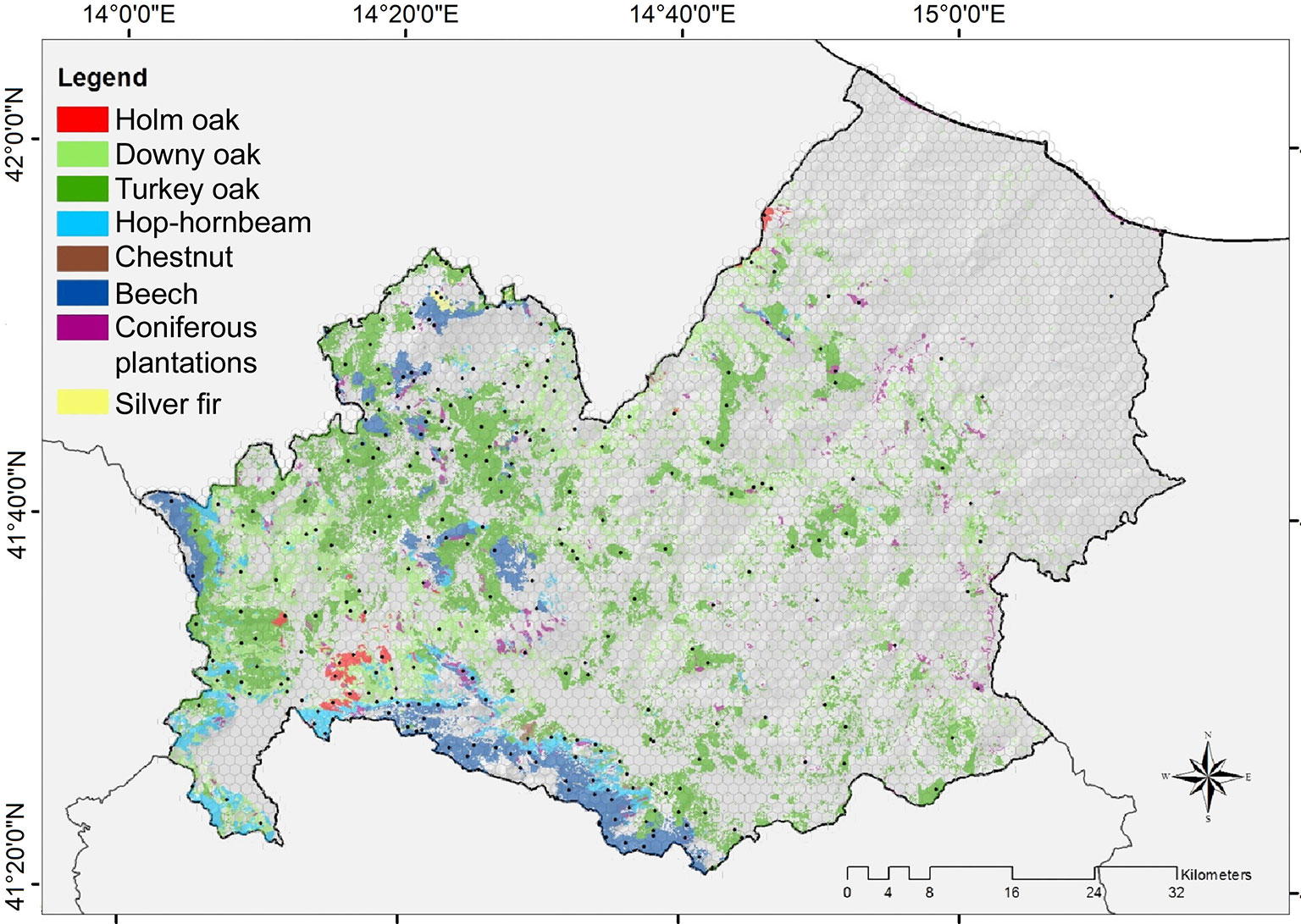
Forests and other wooded lands cover 35% of the region and are dominated by deciduous broad-leaved formations ([31]). Turkey oak forests (Quercus cerris) represent the most common forest type in this region, covering 40% of the total forest area. In some hilly warm sectors, downy oaks (Quercus pubescens) dominate the forest landscape (22% of forests). In mountain sectors (above 1200 m a.s.l.) and at colder sites, deciduous oak forests are replaced by beech forests (Fagus sylvatica - 9.5% of the forest area). Other forest categories which are less represented include the hop-hornbeam forests (Ostrya carpinifolia), holm oak forests (Quercus ilex) and chestnut forests (Castanea sativa). The autochthonous silver-fir forest (Abies alba, 0.3% of the forest area) is of particular interest because it represents a post-glacial relict that only survives in small areas of the Apennines ([43], [65]). Most forests in this region are even-aged (128 402 ha, approximately 80% of the total forest area in the region), and are mainly managed as coppice for the production of firewood. In unmanaged areas, open formations and irregular structured forests (e.g., invasive broad-leaved forests and riparian forests) are also present ([31]).

In this study we used cloud free IRS LISS III imagery acquired in the summer of 2006 for predicting the growing stock volume. Imagery was obtained from the IMAGE2006 dataset ([54]). The imagery was characterized by several salient features: (i) geometrically and radiometrically corrected; (ii) nominal spatial resolution of 23.5 meters resampled at 20 m through a cubic convolution resampling and projected in WGS 84 UTM 32N; and (iii) four bands acquired between the green and near infrared wavelengths (0.52-0.59 µm, 0.62-0.68 µm, 0.77-0.86 µm, 1.55-1.70 µm). A more detailed description is reported by Müller et al. ([54]).

A map of the even-aged forest categories in the region was obtained from a fine scale (1:10.000) map of forest types ([31]). We selected the following eight even-aged categories: (i) holm oak forests; (ii) downy oak forests; (iii) hop-hornbeam forests; (iv) chestnut forests; (v) turkey oak forests; (vi) beech forests; (vii) coniferous plantations (coastal/plain coniferous plantations and mountainous/sub-mountainous coniferous plantations); (viii) silver-fir forests (Fig. 1). Geocoded field data regarding the growing stock volume was collected in the framework of a regional Forest Inventory carried out in 2006. The Forest Inventory was conducted using a standard two-phase tessellated random-stratified sampling (TSS) design (see [18] and [25] for details). All tree stems with a diameter at breast height (DBH) greater than 3 cm were calipered in 304 circular plots having a radius of 13 m. In addition, tree height was measured for a subsample of these trees following the Italian National Forest Inventory protocol ([40]) and then estimated for the rest of the trees. For each sampling unit, the growing stock volume was calculated using allometric equations which were based on stem DBH and height ([10]).

Inverted yield models

Yield refers to the final dimensions of a forest variable (e.g., growing stock volume or annual increment) at the end of a certain period ([70]). In even-aged stands, yield equations predict the growing stock volume (GS) at a specified age (eqn. 1):

As a consequence, an inverted yield equation can be used to estimate the forest stand age as a function of growing stock (eqn. 2):

Here, for each even-aged forest category, we selected a yield equation specifically developed for the Molise region or, when this was not available, we selected an equation build up for different areas in central Italy having forest stand characteristics similar to those of the study area. Next, the yield equations (GS-age functions) were inverted to determine the age at a given GS volume (inverted yield equations). A full description of the equations used in this study is reported in the Appendix 1.

Local standwise forest inventories

To assess the accuracy of the forest growing stock volume and stand age spatial predictions, we used an independent dataset containing information about the growing stock and stand age. To this purpose, we created a geodatabase by aggregating 21 local standwise forest inventories which were available in the study area. The information in these inventories is available for each forest stand. The growing stock volume in the forest management units was measured on the basis of specific sample plots or on the basis of full calipering. Stand age was measured as the number of years from the last disturbance (in most of the cases the last harvesting event). This information was considered free of errors for the subsequent steps of our work.

The information recorded in the plans refers to the year of plan preparation. We updated the growing stock volumes to 2006 (the same of satellite images), using the mean annual increments derived from the yield models. The forest age of each forest unit was also updated by adding the number of years intervening between the year of preparation of the inventory and the year 2006. Finally, we excluded all management units with silvicultural interventions occurred between the plan date and the year 2006. Overall, the growing stock volume information was available for 446 stand units, covering an area of 4959 ha, and ranging in size between 0.14 and 52 ha (with a standard deviation of almost 8 ha) The mean actualized growing stock volume per stand unit was 2746.24 m³ (237 m³ ha^-1) and varied between a minimum of 7.02 m³ (10 m³ ha^-1) and a maximum of 16 670 m³ (673 m³ ha^-1) with a standard deviation of 2792 m³ (144 m³ ha^-1). Data regarding forest stand age was available for 305 stand units covering 3137 ha. The mean stand age referred to the year 2006 was 52 years, varying between 1 and 127 years (standard deviation of 35 years).

  Methods 

Forest age was mapped following the general framework outlined in Fig. 2, first by spatially estimating the growing stock volume using the k-NN method, and then by applying the inverted yield models to derive the forest stand age.

Fig. 2 - Flowchart representing the different steps of the proposed procedure for mapping forest age.

  Enlarge/Shrink   Download   Full Width  Open in Viewer

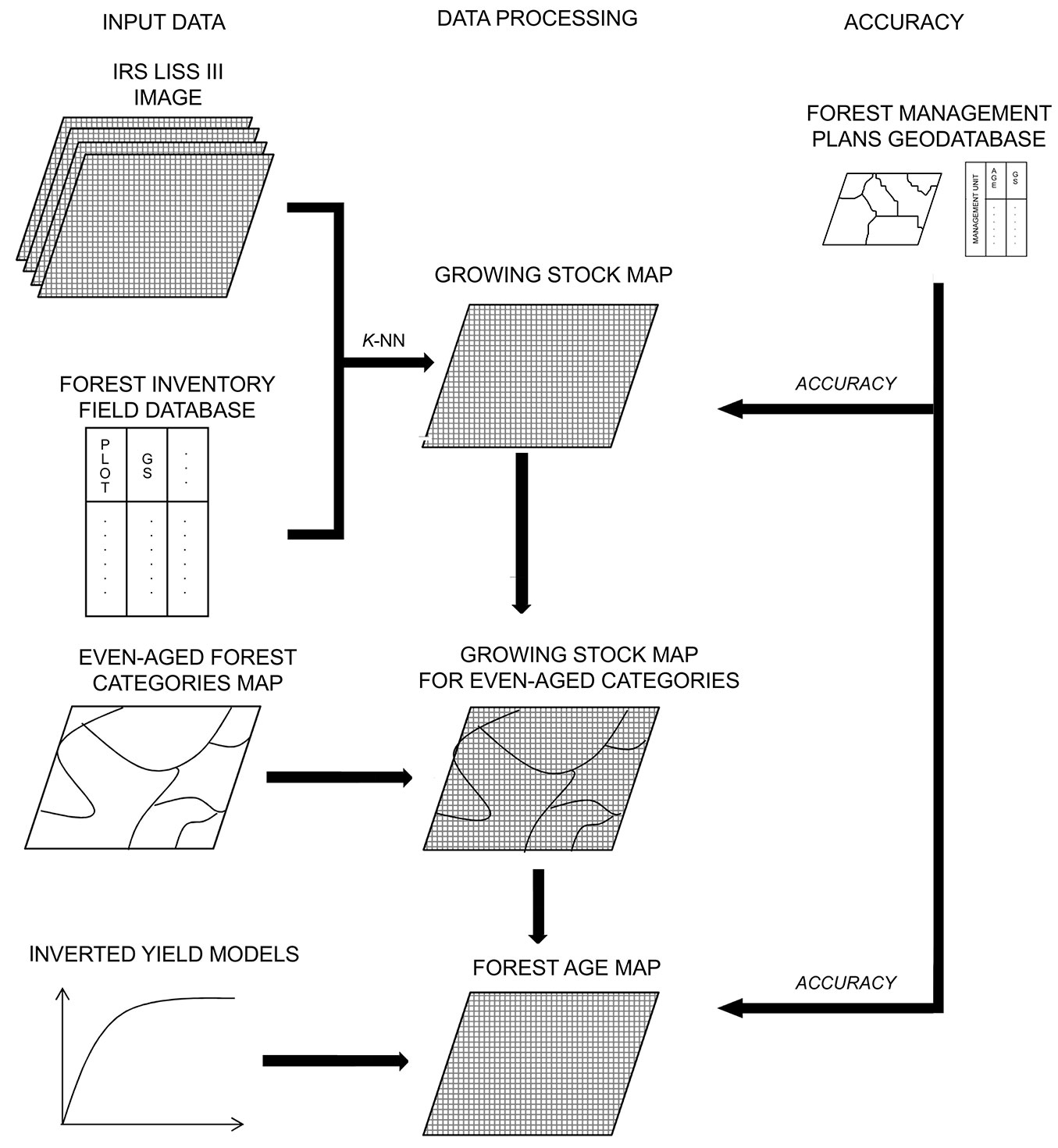
Growing stock map

The non-parametric multivariate k-Nearest Neighbor (k-NN) method was used to spatially estimate the growing stock volume by combining the data acquired at the 304 field plots of the local forest inventory with the IRS LISS III multispectral images ([11], [42]). We estimated the growing stock for each IRS LISS III pixel (GS_t) as follows. The reference pixel set (r) is those for which the IRS LISS III spectral values and the growing stock values (GS_r) observed in the field were available, while the target pixels (t) are those for which the spectral values were available and the growing stock volume (denoted as the target variable GS_t) had to be estimated (eqn. 3):

where GS_rNN represents the growing stock values for the pixels located in the k-Nearest Neighbor sampling units of the target pixel t and W is a weight factor which is inversely related to the distance between the pixel t and the nearest r measured on the fourth dimensional IRS LISS III spectral band space ([12]). Here, the target set was made of the IRS LISS III pixels belonging to the even-aged for- est area (128 402 ha corresponding to 3 210 050 pixels), and the reference was 304 pixels, belonging to the field plots of the local forest inventory. The estimates were calculated using the K-NN FOREST free software ([15]). We tested three different distance measures implemented within the K-NN FOREST software (Euclidean, Mahalanobis and Fuzzy), with k values ranging from 1 to 10 based on the averaged spectral values of a 3 × 3 pixels area surrounding the field plots ([12]). The Leave-One-Out (LOO) approach ([26], [15]) was used to test several k-NN configuration, achieving the most accurate estimation using the Euclidean distance with k= 6.

For a more detailed description of the k-NN algorithm and the assumptions and the implications related to its use, we refer to the vast bibliography available ([12], [2], [50]).

Forest age map

The forest age map was derived on the basis of the growing stock volume map, the map of forest types and the respective inverted yield equations. For each pixel belonging to one of the eight even-aged forest categories considered, we calculated the forest age as a function of growing stock volume by applying the specific inverted yield equations reported in the Appendix 1.

Accuracy assessment

To test the accuracy of the produced maps (firstly growing stock volume and secondly the stand age), the per-pixel estimated values were averaged for each one of the stand units from the standwise forest inventories (446 units for the growing stock volume and 305 units for the stand age). Next, the average values estimated per units were compared against the field-recorded data by calculating the Pearson’s correlation coefficient and the Root Mean Square Errors (RMSE) both in absolute and relative terms.

  Results 

The growing stock volume was accurately estimated through the k-NN process, as the Pearson’s correlation coefficient between estimates and field recorded values per management unit was 0.98, with a RMSE of 22% (Fig. 3a). The estimated mean volume per management unit was 2715 m³, with a range of 0.001-16 724 m³ and a standard deviation (SD) of 2855 m³.

Fig. 3 - Correlation between the predicted and observed (for 446 stand units) total growing stock volume (a) and average age (b). The bold lines represent y=x. Dashed lines indicate the 95% confidence intervals.

  Enlarge/Shrink   Download   Full Width  Open in Viewer

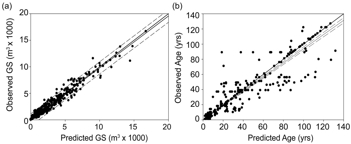
The forest age map (Fig. 4) also resulted accurate (Fig. 3b), with a correlation between estimated and observed age (per forest management unit) of 0.928 and a RMSE of 15.78 years (30% of the real values). The estimated forest age per-pixel varied between 1 and 200 years, with a mean of 33 years (± 24 SD - Fig. 5).

Fig. 4 - Forest age distribution in the Molise region for even-aged categories.

  Enlarge/Shrink   Download   Full Width  Open in Viewer

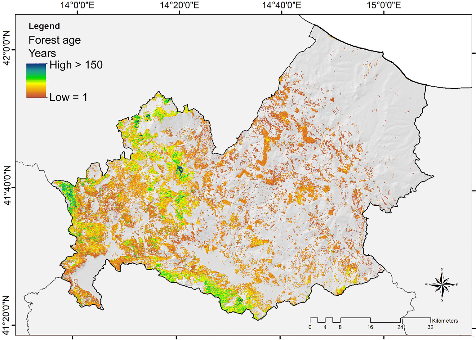
Fig. 5 - Mean estimated forest age (white circle) for the eight even-aged forest types with their respective standard deviations (whiskers). The continuous horizontal line refers to the average age of forests in the region, while the dashed lines represent the regional standard errors. The grey bars represent the area (in ha) covered by each forest type.

  Enlarge/Shrink   Download   Full Width  Open in Viewer

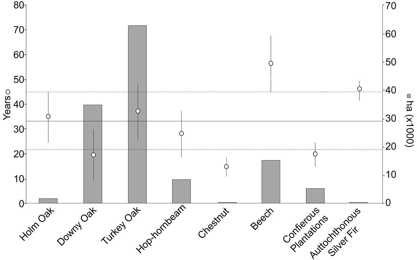
Beech and autochthonous silver-fir forests resulted as the oldest formations, with average ages of 56 ± 24 and 46 ± 10 years, respectively. In contrast, chestnut forests (15 ± 8 years) resulted the youngest forests. The downy oak forests and coniferous plantations were relatively young with 19 ± 21 and 20 ± 9 years, respectively. The remaining deciduous broadleaved forests (Holm and Turkey oaks, and Hop-hornbeam forests) had mean ages similar to the entire forested area (35 ± 20, 37 ± 23 and 28 ± 18, respectively).

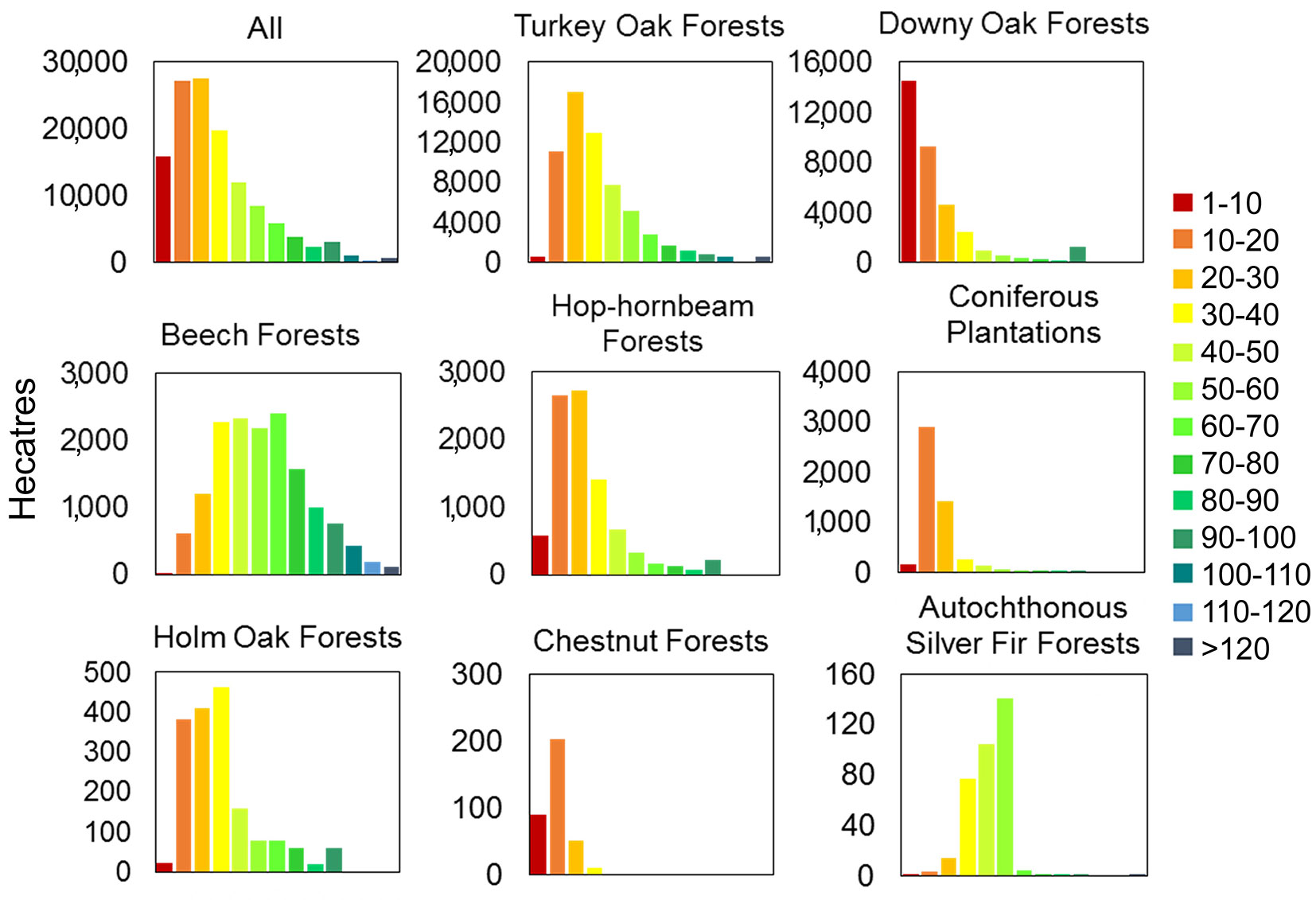
After subdividing the forest age map in ten-year classes, we found that 34% of the investigated forests were less than 20 years old, 60% were between 20 and 80 years old and only the 6% of the forests were older than 80 years (Fig. 6). Only 0.56% of the forests were older than 120 years and only 0.29% older than 140 years. The oldest age class (190-200) was rare, with a percentage of 0.02%. The dominant age classes were 10-20 and 20-30, representing approximately 43% of the investigated forested area. Some forests were mainly distributed in young formations within the region. For example, most coniferous plantations were younger than 10 years, while the downy oak forests and the chestnut forests were largely represented by stands of 10 to 20 years. Turkey oak, hop-hornbeam and holm oak forests were more abundant in the young-middle-aged classes (10-40 years) and were less represented in older stands. For turkey oak and hop-hornbeam forests, the age class of 20-30 years was dominant, while 30-40 years was the dominant age class for the holm oak forests. Beech forests follow a bell-shaped distribution with the majority of forests occurring in the age group of 30-70 years and a maximum age group of 60-70 years. In contrast, most silver fir forests were between 50 and 60 years old, though some younger stands were present.

Fig. 6 - Forest cover extension (hectares) for each category, according to the estimated age (10-year intervals).

  Enlarge/Shrink   Download   Full Width  Open in Viewer

  Discussion 

The relatively young age of the mapped forests (43% of the forest area in our study ranges between 10 and 30 years) reflects the management practices in the studied region, where coppice with short rotation periods (usually less than 25 years) is the most common silvicultural system for broadleaves ([17]). This management type is widespread over the Italian peninsula, particularly along the Apennines, and accounts for approximately 3.9 million of hectares, almost 40% of the total forest area in Italy ([39]). Contrastingly, approximately 0.5% of the forests in the study region are older than 140 years (mainly represented by beech and turkey oak forests). Although such percentage is lower than that reported for Central European forests ([28]), it will likely increase in the near future, mainly as a consequence of the abandonment of traditional harvesting and silvicultural practices which progressively occurred since the end of the second World War. Indeed, a gradual increase in forest age ([71]), cover ([32], [27]), and growing stock volume ([69]) was already observed in Europe.

The oldest formations in the study area are beech forests, mainly managed by the shelterwood system and only marginally as coppices with longer rotation periods (30-40 years) as compared with other broadleaves. Such areas are mainly located in the less accessible upper mountain belt, where traditional silvicultural activities were abandoned as a result of depopulation and socio-economic changes. Consequently, these older beech forests are undergoing natural evolution ([17], [8], [44]). Furthermore, the conversion of coppices into high forests has been implemented in the last few decades in hilly and mountainous Mediterranean beech forests to attenuate the negative effects of frequent clearcuttings on the soil, landscape and biodiversity ([17], [56]). This will also contribute to increase the forest age in the next future across the studied area.

On the contrary, oak forests were relatively younger as a result of the traditional coppicing (clearcut with rotation period of 18-25 years) extensively applied for fuel wood production ([16]). However, turkey oak forests tend to be older than downy oak forests in the study area. In fact, turkey oak typically grows in hilly and sub-mountain areas, where coppice stands lost their economic importance and were abandoned to natural evolution or even converted to high forests ([56]). These less accessible stands are now ageing and resulted older than their traditional rotation period (more than 25 years). Contrastingly, downy oak forests are located in the hilly sector of the Mediterranean bioclimatic zone, where the anthropic exploitation is more intense due to their easier access ([7], [1]). These forests are regularly clear-cut, and consequently old stands are not present.

Both Holm oak and hop-hornbeam forests, which were traditionally grazed or coppiced for coal and fuel wood production ([7]), are currently present in the studied area with young and middle aged stands. As in the cases of oak forests, young stands are located in more accessible areas, while older stands are typically limited to less accessible and remote districts.

Young and small coniferous plantations dominated by Pinus nigra and Pinus pinaster are widespread in the Molise region. Coniferous plantations were introduced in the 1960s, mainly for protecting against soil erosion ([31]). It is likely that the stand age map produced in this study underestimated the real age of such forests as they were planted on very poor and rocky soils, thus leading to a diminished stand growth rate. As a consequence, their current standing volume is probably lower that that expected based on the application of the yield models adopted in this study.

Chestnut forests were generally very young (between 10 and 20 years) and of limited extent (less than 360 ha). In the region, chestnut is mainly managed as coppice (frequently with short rotation periods of less than 20 years) for wood pole production ([31]). Finally, autochthonous silver fir forests have a very limited extension in the region (less than 350 ha) and were mainly present in middle-aged classes, revealing their past management history based on clear-cuttings. Nowadays, the traditional forest management of these pure Abies alba stands is abandoned both for the lack of economic interest in their wood assortments ([65]) and their high conservation value ([44]). For the above reasons, the age of these stands will likely increase in the future as a result of their current natural evolution.

In this study we produced a forest age map through the application of inverted yield models to a growing stock volume map created by integrating field data and remotely-sensed images though the k-NN method. The final map of forest stand age showed a good accuracy, giving an overall RMSE of 30% which is in line with previous experiences developed for mapping forest variables ([63], [52]). The method we propose does not use stand age measurements acquired in the field. Age maps produced from detailed inventory data ([63]) and different source of data containing information on historical forest disturbance ([58]) may have high accuracy. However, such methods may be not implemented in areas where spatially distributed inventory plots are not available, as well as where inconsistencies between different data source exists, or when forest age is not provided by national or local inventories ([51]). In order to avoid these inconsistencies, in this work stand age was instead calculated on the basis of growing stock volume, which is a fairly well standardized variable across different countries, or at least it can be easily harmonized ([51]). As a consequence, our approach can be used for aggregating plot level information from NFIs of different countries, avoiding the problem of merging stand age information which refer to different definitions ([53]).

First attempts to construct forest age map in European countries have been carried out ([3], [67], [71]). Although these studies were extremely useful in depicting forest age structure in Europe, the achieved results were mainly useful when aggregated at national level. For example, the maps produced by Vilén et al. ([71]) were in fact very coarse as for their spatial resolution (0.25°), being based on the simplistic assumption of a homogenous distribution of all age classes over the forest area in a country. In other words, the distribution of forest age classes available from National Forest Inventories of a given country are considered invariant in all the forest area of that country. On the contrary, our map has a geometric resolution of 20 m and could be a useful tool for planning local forest management actions. Nevertheless, it is advisable to use the produced forest age map at much coarser level since k-NN estimations could have a low pixel based accuracy ([63]). However, in our case the map accuracy (and thus its usefulness) dramatically improve when the estimations are aggregated over larger areas such as stands or management levels. In this respect and despite the limitations due to the use of an opportunistic database for accuracy assessment (e.g., nonprobability sampling design - [57]), the use of local standwise forest inventories was considered acceptable here for the following reasons: (i) the dataset is entirely independent from the dataset used for GS map production; and (ii) it is cost-effective ([57]).

A stand age high-resolution map may have different uses. Firstly, such information can provide a sound basis for orienting forest management strategies, such as facilitating a general assessment of harvesting potential, identifying suitable stands to be promoted to natural evolution, or contributing to determining the optimal forest management strategies and maximizing the productivity of different ecosystem services. Secondly, forest age maps provide important, quantitative information supporting the assessment of carbon sequestration of forest ecosystems and their role in biogeochemical cycles ([34]). For example, younger stands are expected to exhibit a rapid increase in Net Primary Productivity (NPP), while older stands are expected to exhibit a slow decline. In this case, the availability of forest age spatial distribution patterns could be useful for assessing potential changes in the NPP under different management scenarios. Thus, potential changes in important ecosystems services which are directly associated with NPP, such as carbon sequestration, water cycling and regulation, soil fertility, local climate and air quality, could be assessed ([75]). Stand age distribution patterns could provide relevant information for monitoring biodiversity and in general for restoring more favorable conditions in old and even-aged forests ([6]). Finally, the proposed method could be a useful tool for supporting the implementation of forest management strategies in those regions where land ownership fragmentation ([60]) or the limited commercial value of timber production led to a lack of local management plans, as frequently occurs in Mediterranean areas.

The method we propose enlarges the range of applicability of yield models ([70]), calling for the development of site-specific equations for main forest categories covering all the main biogeographical regions of Europe ([72], [59]). Yield models were the oldest approach to yield estimations and their development was based on several assumptions that limit their range of applicability ([72], [73]). For example, yield models assume that the age-volume relationship is valid for fully stocked or “normal” forest stands under specific stand site characteristics (e.g., soil fertility). When such models were locally unavailable for a specific forest type, those available for a neighboring region were adopted. All these issues lessen the accuracy of estimates. Future development of site-specific equations will likely enhance the proposed approach.

The main limitations of our approach is its suitability for age prediction of even-aged forests, which in any case represent the large majority of forests in the study area (80%). Similarly, based on data from the last “State of Europe’s forests” ([28]) for 18 European countries (including the Russian Federation), even-aged forests represent the vast majority of European forests (almost 90%, with more than 9 million of hectares). For such reason, the proposed method has a potential relevance for applications at the pan-European level.

  Conclusions 

In this study a simple and straightforward method for spatially estimating forest age was implemented through the application of inverted yield models to a growing stock volume map created by integrating field data and remotely-sensed images though the k-NN method. We produced a forest stand age map covering 128 402 ha with an accuracy (RMSE of 30%) which is in line with previous experiences developed for mapping forest variables.

The increasing development of Earth Observation techniques and the availability of forest inventories may probably lead to a more habitual derivation of forest variables maps in the near future. The procedure adopted in this study may be applied to European forests at continental scales on the basis of the information already available, for example based on the growing stock volume map from Gallaun et al. ([29]), and the forest species map from Brus et al. ([5]). This is particularly important as forest conservation across Europe requires a common approach to define and map forest age. Therefore, we advocate further studies to be conducted in the future to properly test and refine this procedure, with the aim of providing integrated information for increasingly larger areas.

  Acknowledgements 

This work was supported by the European Commission under the project by the LIFE+ ManFor C.BD (Life Environment Project LIFE09 ENV/IT/000078) and by the Italian Ministry of University and Research in the framework of the following projects: “Development of innovative methods for forest ecosystems monitoring based on remote sensing” (PRIN2012 - grant no. 2012EWEY2S); CARBOTREE (PRIN2011 - grant no. B21J12000560001); “Sviluppo di modelli innovativi per il monitoraggio multiscala degli indicatori di servizi ecosistemici nelle foreste Mediterranee” (FIRB2012 - grant no. RBFR121TWX); and NEUFOR (PRIN2012 - grant no. 2012K3A2HJ]. We gratefully acknowledge two anonymous referees for valuable comments on the original version of the manuscript.

  References

  Supplementary Material

Tab. S1 - Inverted yield equations used for forest age estimation.